Effects of QCD radiation on inclusive variables for determining the scale of new physics at hadron colliders

Abstract:

We examine the effects of QCD initial-state radiation on a class of quantities, designed to probe the mass scale of new physics at hadron colliders, which involve longitudinal as well as transverse final-state momenta. In particular, we derive universal functions that relate the invariant mass and energy distribution of the visible part of the final state to that of the underlying hard subprocess. Knowledge of this relationship may assist in checking hypotheses about new processes, by providing additional information about their scales. We compare our results with those of Monte Carlo studies and find good general agreement.

1 Introduction

Searching for new physics at hadron colliders is difficult, partly because of the complexity of the expected new signals (typically, multiple jets and/or leptons plus missing energy) but also because processes at high mass scales are accompanied by copious initial-state QCD radiation (ISR). As this tends to be emitted close to the incoming beam directions, and the longitudinal momentum of the hard subprocess is anyway unknown, search variables [1, 2, 3, 4, 5, 6, 7, 8, 9, 10, 11, 12, 13, 14, 15, 16, 17, 18, 19, 20, 21, 22, 23, 24, 25, 26, 27, 28, 29, 30, 31, 32, 33, 34, 35, 36, 37, 38, 39, 40, 41] have generally been constructed either from the transverse components of observed final-state momenta or else by assuming that some subset of these momenta can be unambiguously ascribed to the hard subprocess. Variables that make use of all observed momenta without hypothesizing any particular structure of the final state are termed global inclusive variables in ref. [41]. Examples of transverse global quantities of this type are the observed transverse energy $E_{T}$, the missing transverse energy $\not\!\!E_{T}$, and their sum $H_{T}=E_{T}+\not\!\!E_{T}$. The distributions of such quantities can provide information on the energy scales of new processes such as supersymmetric particle production [1, 2, 6].

Although the longitudinal components of final-state momenta are strongly influenced by ISR, they do contain information about the underlying hard subprocess. Indeed, the amount of ISR emitted is determined by the energy scale of the subprocess. It is therefore of interest to quantify the effects of ISR on global observables that involve longitudinal momentum components. The aim of the present paper is to take the first steps in that direction.

In ref. [41] various global search variables were investigated, including those that make use of longitudinal as well as transverse momentum components. The quantities studied included the total energy $E$ visible in the detector and the visible invariant mass $M$,

$$M=\sqrt{E^{2}-P_{z}^{2}-\not\!\!E_{T}^{2}}$$ (1)

where $P_{z}$ is the visible longitudinal momentum. In addition a new variable was introduced, defined as

$$\hat{s}^{1/2}_{\rm min}(M_{\rm inv})\equiv\sqrt{M^{2}+\not\!\!E_{T}^{2}}+\sqrt{M_{\rm inv}^{2}+\not\!\!E_{T}^{2}}\ ,$$ (2)

where the parameter $M_{\rm inv}$ is a variable estimating the sum of masses of all invisible particles in the event:

$$M_{\rm inv}\equiv\sum_{i=1}^{n_{\rm inv}}m_{i}\ .$$ (3)

It was argued that the peak in the distribution of $\hat{s}^{1/2}_{\rm min}$ is a good indicator of the mass scale of new physics processes involving heavy particle production.

It will also be useful to define the rapidity of the visible system,

$$Y\equiv\frac{1}{2}\ln\left(\frac{E+P_{z}}{E-P_{z}}\right)\ .$$ (4)

The present paper examines the effects of ISR on global inclusive search variables, first in an approximate fixed-order treatment taking into account collinear-enhanced terms, and then in an all-orders resummation of such terms. We quantify the way the distributions of quantities that involve longitudinal momenta depend on the scale of the underlying hard subprocess and on the properties of the detector, in particular the maximum visible pseudorapidity $\eta_{\rm max}$. With the insight thus gained, it may be possible to correct for this dependence and thereby extract information on the hard subprocess from such quantities.

2 Fixed-order analysis

The Monte Carlo results presented in ref. [41] show that the second term on the right-hand side of eq. (2) is not strongly affected by ISR. The first term is intended to add extra longitudinal information about the hard subprocess, allowing a more reliable determination of its mass scale. The extra longitudinal information enters through the visible mass $M$. We therefore concentrate mainly on this quantity.

2.1 Born approximation

Since the effect of invisible final-state particles is not the central issue here, let us suppose first that all the final-state particles from the hard subprocess are detected. Then in Born approximation, assuming that no beam remnants are detected, $M$ yields a perfect estimate of the centre-of-mass energy of the hard subprocess. For incoming partons with momentum fractions $x_{1,2}$,

$$E=\frac{1}{2}\sqrt{S}(x_{1}+x_{2})\;,\;\;\;P_{z}=\frac{1}{2}\sqrt{S}(x_{1}-x_{2})\;,$$ (5)

where $\sqrt{S}$ is the hadron-hadron centre-of-mass energy, so that

$$M^{2}=x_{1}x_{2}S\;,\;\;\;Y=\frac{1}{2}\ln\frac{x_{1}}{x_{2}}\ .$$ (6)

The differential cross section for parton flavours $a,b$ is thus

$$\frac{d\sigma_{ab}}{dM^{2}dY}=\int dx_{1}\,dx_{2}\,f_{a}(x_{1})f_{b}(x_{2})\delta(M^{2}-x_{1}x_{2}S)\delta\left(Y-\frac{1}{2}\ln\frac{x_{1}}{x_{2}}\right)\hat{\sigma}_{ab}(x_{1}x_{2}S)$$ (7)

where $f_{a,b}$ are the relevant parton distribution functions for the incoming hadrons and $\hat{\sigma}_{ab}$ is the hard subprocess cross section. Hence at Born level we find

$$S\frac{d\sigma_{ab}}{dM^{2}dY}=f_{a}\left(\frac{M}{\sqrt{S}}e^{Y}\right)f_{b}\left(\frac{M}{\sqrt{S}}e^{-Y}\right)\hat{\sigma}_{ab}(M^{2})\ .$$ (8)

The parton distributions are normally given as $F_{i}(x)=xf_{i}(x)$, in terms of which we have

$$M^{2}\frac{d\sigma_{ab}}{dM^{2}dY}=F_{a}\left(\frac{M}{\sqrt{S}}e^{Y}\right)F_{b}\left(\frac{M}{\sqrt{S}}e^{-Y}\right)\hat{\sigma}_{ab}(M^{2})\ .$$ (9)

If the partonic cross section $\hat{\sigma}_{ab}$ has a threshold or peak, indicating that the $ab$ subprocess has a characteristic scale $Q$, then this is also manifest in the Born cross section (9) at $M\sim Q$, provided the relevant parton distributions are large enough for that subprocess to contribute significantly.

From eqs. (5) and (6) we have $E=M\cosh Y$ and therefore the visible energy distribution is given in Born approximation by

$$E^{2}\frac{d\sigma_{ab}}{dE^{2}dY}=\left.M^{2}\frac{d\sigma_{ab}}{dM^{2}dY}\right|_{M=E\,\mbox{\scriptsize sech}\,Y}\ .$$ (10)

2.2 Quasi-collinear NLO correction

To examine the sensitivity of the above results to ISR, let us first compute the NLO contribution due to quasi-collinear gluon emission and the associated virtual corrections. Consider first the emission of a gluon from parton $a$. If the emission angle $\theta$ is large enough, say $\theta>\theta_{c}$, the gluon enters the detector and contributes to $M$. In the small-angle approximation we then have

$$E=\frac{1}{2}\sqrt{S}(x_{1}/z+x_{2})\;,\;\;\;P_{z}=\frac{1}{2}\sqrt{S}(x_{1}/z-x_{2})\;,$$ (11)

where $x_{1}/z$ is the momentum fraction of parton $a$ before the emission, so that

$$M^{2}=x_{1}x_{2}S/z\;,\;\;\;Y=\frac{1}{2}\ln\frac{x_{1}}{zx_{2}}\ .$$ (12)

The correction associated with a detected emission from parton $a$ is then

$$\frac{\alpha_{\rm S}}{\pi}\int_{\theta_{c}}\frac{d\theta}{\theta}\frac{dz}{z}dx_{1}\,dx_{2}\tilde{P}_{a}(z)f_{a}(x_{1}/z)f_{b}(x_{2})\delta(M^{2}-x_{1}x_{2}S/z)\delta\left(Y-\frac{1}{2}\ln\frac{x_{1}}{zx_{2}}\right)\hat{\sigma}_{ab}(x_{1}x_{2}S)$$ (13)

where $\tilde{P}_{a}(z)$ is the unregularized $a\to ag$ splitting function.

On the other hand if the gluon misses the detector ($\theta<\theta_{c}$), $E$ and $P_{z}$ are still given by (5), so the contribution is

$$\frac{\alpha_{\rm S}}{\pi}\int_{0}^{\theta_{c}}\frac{d\theta}{\theta}\frac{dz}{z}dx_{1}\,dx_{2}\tilde{P}_{a}(z)f_{a}(x_{1}/z)f_{b}(x_{2})\delta(M^{2}-x_{1}x_{2}S)\delta\left(Y-\frac{1}{2}\ln\frac{x_{1}}{x_{2}}\right)\hat{\sigma}_{ab}(x_{1}x_{2}S)\,.$$ (14)

Finally the associated virtual correction is the term that regularizes the splitting function, which in this approximation is

$$-\frac{\alpha_{\rm S}}{\pi}\int\frac{d\theta}{\theta}\,dz\,dx_{1}\,dx_{2}\tilde{P}_{a}(z)f_{a}(x_{1})f_{b}(x_{2})\delta(M^{2}-x_{1}x_{2}S)\delta\left(Y-\frac{1}{2}\ln\frac{x_{1}}{x_{2}}\right)\hat{\sigma}_{ab}(x_{1}x_{2}S)\,.$$ (15)

Adding everything together gives a correction

$$\delta\left(\frac{d\sigma_{ab}}{dM^{2}dY}\right) = \frac{\alpha_{\rm S}}{\pi}\int\frac{d\theta}{\theta}\,dz\,dx_{1}\,dx_{2}\,\tilde{P}_{a}(z)f_{b}(x_{2})\hat{\sigma}_{ab}(x_{1}x_{2}S)$$

$$\Bigl{[}\frac{1}{z}f_{a}(x_{1}/z)\delta\left(Y-\frac{1}{2}\ln\frac{x_{1}}{zx_{2}}\right)\delta(M^{2}-x_{1}x_{2}S/z)\Theta(\theta-\theta_{c})$$

$$+\Bigl{\{}\frac{1}{z}f_{a}(x_{1}/z)\Theta(\theta_{c}-\theta)-f_{a}(x_{1})\Bigr{\}}\delta\left(Y-\frac{1}{2}\ln\frac{x_{1}}{x_{2}}\right)\delta(M^{2}-x_{1}x_{2}S)\Bigr{]}\ .$$

Setting aside for the moment the possibility of splittings other than $a\to ag$, the DGLAP evolution equation for $f_{a}(x_{1})$ is

$$q\frac{\partial}{\partial q}f_{a}(x_{1})=\frac{\alpha_{\rm S}}{\pi}\int dz\,\tilde{P}_{a}(z)\left[\frac{1}{z}f_{a}(x_{1}/z)-f_{a}(x_{1})\right]$$ (17)

where $q$ represents the scale at which the parton distribution is measured. Hence the correction may be written as

$$\delta\left(\frac{d\sigma_{ab}}{dM^{2}dY}\right) = \int\frac{d\theta}{\theta}\,dx_{1}\,dx_{2}\,f_{b}(x_{2})\hat{\sigma}_{ab}(x_{1}x_{2}S)\Biggl{[}q\frac{\partial f_{a}}{\partial q}\delta\left(Y-\frac{1}{2}\ln\frac{x_{1}}{x_{2}}\right)\delta(M^{2}-x_{1}x_{2}S)$$ (18)

$$+\frac{\alpha_{\rm S}}{\pi}\int\frac{dz}{z}\tilde{P}_{a}(z)\,f_{a}(x_{1}/z)\Biggl{\{}\delta\left(Y-\frac{1}{2}\ln\frac{x_{1}}{zx_{2}}\right)\delta(M^{2}-x_{1}x_{2}S/z)$$

$$-\delta\left(Y-\frac{1}{2}\ln\frac{x_{1}}{x_{2}}\right)\delta(M^{2}-x_{1}x_{2}S)\Biggr{\}}\Theta(\theta-\theta_{c})\Biggr{]}\ .$$

Since $d\theta/\theta=dq/q$, the first term represents a change of scale in the Born term. It replaces the reference scale in $f_{a}$ by the scale $Q$ of the hard subprocess. The remaining terms give a correction

$$\delta\left(\frac{d\sigma_{ab}}{dM^{2}dY}\right) = \frac{\alpha_{\rm S}}{\pi S}\int_{\theta_{c}}\frac{d\theta}{\theta}\int\frac{dz}{z}\tilde{P}_{a}(z)f_{b}\left(\frac{M}{\sqrt{S}}e^{-Y}\right)\times$$ (19)

$$\left[f_{a}\left(\frac{M}{\sqrt{S}}e^{Y}\right)z\hat{\sigma}_{ab}(zM^{2})-f_{a}\left(\frac{M}{z\sqrt{S}}e^{Y}\right)\hat{\sigma}_{ab}(M^{2})\right]\ .$$

In leading-log approximation the $\theta$ integration just gives a factor of $-\ln\theta_{c}$. In the same approximation, we may set $-\ln\theta_{c}=\eta_{\rm max}$, the maximum pseudorapidity seen by the detector. Note that this is a different quantity from $Y$, the true rapidity of the visible system, given by eq. (4). The correction associated with parton $b$ gives the same expression with $a\leftrightarrow b$ and $Y\to-Y$. Thus, defining

$$\bar{x}_{1}=\frac{M}{\sqrt{S}}e^{Y}\;,\;\;\;\bar{x}_{2}=\frac{M}{\sqrt{S}}e^{-Y}\;,$$ (20)

we have

$$S\frac{d\sigma_{ab}}{dM^{2}dY} = f_{a}(\bar{x}_{1},Q)f_{b}(\bar{x}_{2},Q)\hat{\sigma}_{ab}(M^{2})$$ (21)

$$+ \eta_{\rm max}\frac{\alpha_{\rm S}}{\pi}\int\frac{dz}{z}\Bigl{[}z\{\tilde{P}_{a}(z)+\tilde{P}_{b}(z)\}f_{a}(\bar{x}_{1},Q)f_{b}(\bar{x}_{2},Q)\hat{\sigma}_{ab}(zM^{2})$$

$$- \{\tilde{P}_{a}(z)f_{a}(\bar{x}_{1}/z,Q)f_{b}(\bar{x}_{2},Q)+\tilde{P}_{b}(z)f_{a}(\bar{x}_{1},Q)f_{b}(\bar{x}_{2}/z,Q)\}\hat{\sigma}_{ab}(M^{2})\Bigr{]}.$$

Expressing this in terms of $F_{i}(x)=xf_{i}(x)$, as in eq. (9),

$$M^{2}\frac{d\sigma_{ab}}{dM^{2}dY} = F_{a}(\bar{x}_{1},Q)F_{b}(\bar{x}_{2},Q)\hat{\sigma}_{ab}(M^{2})$$

$$+ \eta_{\rm max}\frac{\alpha_{\rm S}}{\pi}\int dz\Bigl{[}\{\tilde{P}_{a}(z)+\tilde{P}_{b}(z)\}F_{a}(\bar{x}_{1},Q)F_{b}(\bar{x}_{2},Q)\hat{\sigma}_{ab}(zM^{2})$$

$$- \{\tilde{P}_{a}(z)F_{a}(\bar{x}_{1}/z,Q)F_{b}(\bar{x}_{2},Q)+\tilde{P}_{b}(z)F_{a}(\bar{x}_{1},Q)F_{b}(\bar{x}_{2}/z,Q)\}\hat{\sigma}_{ab}(M^{2})\Bigr{]}\ .$$

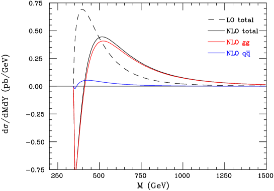
Results for $t\bar{t}$ production at the LHC ($pp$ at $\sqrt{S}=14$ TeV) with $\eta_{\rm max}=5$ and $Y=0$ are shown in fig. 1. Leading-order MSTW parton distributions [42] were used. For simplicity we have taken $Q=M$. Recall that the simplifying assumption made here is that all $t\bar{t}$ decay products are detected, so the $M$ distribution vanishes below $t\bar{t}$ threshold. We see that there is a large negative NLO correction near threshold, followed by a broad positive peak.

Figure 1: Distribution of visible mass $M$ in $t\bar{t}$ production at LHC for $\eta_{\rm max}=5$ and $Y=0$: leading and approximate next-to-leading order.

To understand these qualitative features, consider the case $a=b$, as in $gg\to t\bar{t}$, and $Y=0$, so that $\bar{x}_{1,2}=M/\sqrt{S}\equiv\bar{x}$. Then the NLO correction becomes simply

$$\delta\left(M^{2}\frac{d\sigma}{dM^{2}dY}\right)=2\eta_{\rm max}\frac{\alpha_{\rm S}}{\pi}F(\bar{x})\int dz\tilde{P}_{a}(z)\left[F(\bar{x})\hat{\sigma}(zM^{2})-F(\bar{x}/z)\hat{\sigma}(M^{2})\right]$$ (23)

The first term is positive-definite, contributes only above threshold, and diverges at threshold. It produces the broad positive peak. The second term is negative-definite, contributes around threshold, and has a divergent coefficient. It provides the sharp negative peak.

From eqs. (11) and (12), the relation $E=M\cosh Y$ still holds in this approximation and therefore the visible energy distribution is again given by eq. (10).

3 Resummation

By adding and subtracting the expression

$$\{\tilde{P}_{a}(z)+\tilde{P}_{b}(z)\}F_{a}(\bar{x}_{1},Q)F_{b}(\bar{x}_{2},Q)\hat{\sigma}_{ab}(M^{2})$$ (24)

in the integrand of eq. (2.2) and comparing with eq. (17), we see that the last line of that equation corresponds to a change of scale $Q\to Q_{c}=\theta_{c}Q$ in the parton distributions, leading to

$$M^{2}\frac{d\sigma_{ab}}{dM^{2}dY}=F_{a}(\bar{x}_{1},Q_{c})F_{b}(\bar{x}_{2},Q_{c})\Sigma_{ab}(M^{2})$$ (25)

where to first order

$$\Sigma_{ab}(M^{2}) = \hat{\sigma}_{ab}(M^{2})$$ (26)

$$+ \eta_{\rm max}\frac{\alpha_{\rm S}}{\pi}\int dz\{\tilde{P}_{a}(z)+\tilde{P}_{b}(z)\}\{\hat{\sigma}_{ab}(zM^{2})-\hat{\sigma}_{ab}(M^{2})\}\;.$$

The interpretation of this result is simple: undetected ISR at angles less than $\theta_{c}$, corresponding to scales less than $\theta_{c}Q$, is absorbed into the structure of the incoming hadrons. To resum the effects of gluons at angles greater than $\theta_{c}$, consider first the real emission of $n$ such gluons from parton $a$. In the quasi-collinear approximation these form an angular-orders sequence, giving rise to a contribution to $\Sigma_{ab}$ of

$$\left(\frac{\alpha_{\rm S}}{\pi}\right)^{n}\int_{\theta_{c}}\frac{d\theta_{1}}{\theta_{1}}\int_{\theta_{1}}\frac{d\theta_{2}}{\theta_{2}}\ldots\int_{\theta_{n-1}}\frac{d\theta_{n}}{\theta_{n}}\int_{0}^{1}dz_{1}\ldots dz_{n}\tilde{P}_{a}(z_{1})\ldots\tilde{P}_{a}(z_{n})\hat{\sigma}_{ab}(z_{1}\ldots z_{n}M^{2})$$

$$=\frac{1}{n!}\left(\eta_{\rm max}\frac{\alpha_{\rm S}}{\pi}\right)^{n}\int_{0}^{1}dz_{1}\ldots dz_{n}\tilde{P}_{a}(z_{1})\ldots\tilde{P}_{a}(z_{n})\hat{\sigma}_{ab}(z_{1}\ldots z_{n}M^{2})\;,$$ (27)

where again we have made the identification $-\ln\theta_{c}=\eta_{\rm max}$. The multiple convolution of the momentum fractions $z_{i}$ can be transformed into a product by taking moments. Defining

$$\int_{0}^{\infty}dM^{2}\left(M^{2}\right)^{-N}\hat{\sigma}_{ab}(M^{2})\equiv\hat{\sigma}^{ab}_{N}$$ (28)

we have

$$\left(\frac{\alpha_{\rm S}}{\pi}\right)^{n}\int_{0}^{\infty}dM^{2}\left(M^{2}\right)^{-N}\int dz_{1}\ldots dz_{n}\tilde{P}_{a}(z_{1})\ldots\tilde{P}_{a}(z_{n})\hat{\sigma}(z_{1}\ldots z_{n}M^{2})=\left(\tilde{\gamma}^{a}_{N}\right)^{n}\hat{\sigma}^{ab}_{N}$$ (29)

where

$$\tilde{\gamma}^{a}_{N}=\frac{\alpha_{\rm S}}{\pi}\int_{0}^{1}dz\,z^{N-1}\tilde{P}_{a}(z)\ .$$ (30)

Therefore defining correspondingly

$$\int_{0}^{\infty}dM^{2}\left(M^{2}\right)^{-N}\Sigma_{ab}(M^{2})\equiv\Sigma^{ab}_{N}\;,$$ (31)

the contribution (3) to this quantity will be

$$\frac{1}{n!}\left(\eta_{\rm max}\tilde{\gamma}^{a}_{N}\right)^{n}\hat{\sigma}^{ab}_{N}$$ (32)

which summed over $n$ gives

$$\exp\left(\eta_{\rm max}\tilde{\gamma}^{a}_{N}\right)\hat{\sigma}^{ab}_{N}\ .$$ (33)

The corresponding virtual contributions give a Sudakov-like form factor

$$\exp\left(-\frac{\alpha_{\rm S}}{\pi}\int_{\theta_{c}}\frac{d\theta}{\theta}\int_{0}^{1}dz\,\tilde{P}_{a}(z)\right)$$ (34)

and therefore the total contribution from parton $a$ is

$$\exp\left(\eta_{\rm max}\gamma^{a}_{N}\right)\hat{\sigma}^{ab}_{N}$$ (35)

where $\gamma^{a}_{N}$ is the anomalous dimension

$$\gamma^{a}_{N}=\frac{\alpha_{\rm S}}{\pi}\int_{0}^{1}dz\left(z^{N-1}-1\right)\tilde{P}_{a}(z)=\frac{\alpha_{\rm S}}{\pi}\int_{0}^{1}dz\,z^{N-1}P_{a}(z)\;,$$ (36)

$P_{a}(z)$ being the regularized $a\to ag$ splitting function. Parton $b$ gives a similar factor with $\gamma^{b}_{N}$ in place of $\gamma^{a}_{N}$, so the result for the quantity (31) is simply

$$\Sigma^{ab}_{N}=e^{\eta_{\rm max}(\gamma^{a}_{N}+\gamma^{b}_{N})}\hat{\sigma}^{ab}_{N}\;.$$ (37)

We can see as follows that this result is qualitatively correct. The anomalous dimensions are positive for small $N$ and negative for large $N$. Thus, for $\theta_{c}\ll 1$, $\Sigma^{ab}_{N}$ is enhanced relative to $\hat{\sigma}^{ab}_{N}$ at small $N$ and suppressed at large $N$. Now from the moment definition (28) small $N$ corresponds to large $M$ and vice versa. Hence the distribution of $M$ is suppressed at small $M$ and enhanced at large $M$ relative to the Born term, as observed in the Monte Carlo [41] and NLO results.

The emission of partons other than gluons is included by introducing the anomalous dimension matrix $\Gamma_{N}$ with elements given by

$$(\Gamma_{N})_{ba}=\frac{\alpha_{\rm S}}{\pi}\int_{0}^{1}dz\,z^{N-1}P_{ba}(z)$$ (38)

where $P_{ba}(z)$ is the regularized $a\to b$ splitting function. Then

$$\Sigma^{ab}_{N}=\hat{\sigma}^{a^{\prime}b^{\prime}}_{N}\left(e^{\eta_{\rm max}\Gamma_{N}}\right)_{a^{\prime}a}\left(e^{\eta_{\rm max}\Gamma_{N}}\right)_{b^{\prime}b}\ .$$ (39)

The corresponding generalization of the evolution equation (17) is

$$q\frac{\partial}{\partial q}f_{b}(x)=\frac{\alpha_{\rm S}}{\pi}\int\frac{dz}{z}P_{ba}(z)f_{a}(x/z)$$ (40)

Defining the moments of the parton distribution functions

$$f^{a}_{N}=\int_{0}^{1}dx\,x^{N-1}f_{a}(x)$$ (41)

we see that

$$q\frac{\partial}{\partial q}f^{b}_{N}=(\Gamma_{N})_{ba}f^{a}_{N}$$ (42)

with solution

$$f^{b}_{N}(q)=\left([q/q_{0}]^{\Gamma_{N}}\right)_{ba}f^{a}_{N}(q_{0})\ .$$ (43)

Hence

$$f^{b}_{N}(Q)=\left(e^{\eta_{\rm max}\Gamma_{N}}\right)_{ba}f^{a}_{N}(Q_{c})\;,$$ (44)

where

$$Q_{c}=\theta_{c}Q=Qe^{-\eta_{\rm max}}\;,$$ (45)

showing that the evolution of the visible mass distribution is related to that of the parton distributions over the same range of scales.

Taking into account the running of the strong coupling $\alpha_{\rm S}(q)$ in the evolution equation (40), eq. (44) becomes

$$f^{b}_{N}(Q)=K^{ba}_{N}f^{a}_{N}(Q_{c})$$ (46)

where

$$K^{ba}_{N}=\left(\left[\frac{\alpha_{\rm S}(Q_{c})}{\alpha_{\rm S}(Q)}\right]^{p\Delta_{N}}\right)_{ba}$$ (47)

with $p=6/(11C_{A}-2n_{f})$ and

$$(\Delta_{N})_{ba}=\frac{\pi}{\alpha_{\rm S}}(\Gamma_{N})_{ba}=\int_{0}^{1}dz\,z^{N-1}P_{ba}(z)\ .$$ (48)

The running of $\alpha_{\rm S}$ will affect eq. (39) similarly, giving

$$\Sigma^{ab}_{N}=\hat{\sigma}^{a^{\prime}b^{\prime}}_{N}K^{a^{\prime}a}_{N}K^{b^{\prime}b}_{N}\ .$$ (49)

This implies that

$$\Sigma_{ab}(M^{2})=\int_{0}^{1}dz\,\hat{\sigma}_{a^{\prime}b^{\prime}}(zM^{2})\,H_{a^{\prime}b^{\prime},ab}(z)$$ (50)

where

$$K^{a^{\prime}a}_{N}K^{b^{\prime}b}_{N}=\int_{0}^{1}dz\,z^{N-1}H_{a^{\prime}b^{\prime},ab}(z)$$ (51)

or, inverting the Mellin transformation,

$$H_{a^{\prime}b^{\prime},ab}(z)=\frac{1}{2\pi i}\int_{C}dN\,z^{-N}K^{a^{\prime}a}_{N}K^{b^{\prime}b}_{N}$$ (52)

where the contour $C$ is to the right of all singularities of the integrand.

Alternatively, eq. (50) can be expressed as a double convolution,

$$\Sigma_{ab}(M^{2})=\int_{0}^{1}dz_{1}\,dz_{2}\,\hat{\sigma}_{a^{\prime}b^{\prime}}(z_{1}z_{2}M^{2})\,K_{a^{\prime}a}(z_{1})\,K_{b^{\prime}b}(z_{2})$$ (53)

where

$$K^{b^{\prime}b}_{N}=\int_{0}^{1}dz\,z^{N-1}K_{b^{\prime}b}(z)\;.$$ (54)

It then follows from eq. (47) that $K_{b^{\prime}b}(z)$ obeys an evolution equation like that of the parton distributions:

$$Q\frac{\partial}{\partial Q}K_{b^{\prime}b}(z)=\frac{\alpha_{\rm S}(Q)}{\pi}\int\frac{dz^{\prime}}{z^{\prime}}P_{b^{\prime}a}(z^{\prime})K_{ab}(z/z^{\prime})\;.$$ (55)

Putting everything together, the visible mass distribution is related to the hard subprocess cross section (in the absence of invisible final-state particles) as follows:

$$M^{2}\frac{d\sigma_{ab}}{dM^{2}dY}=\int dz_{1}\,dz_{2}\,\hat{\sigma}_{a^{\prime}b^{\prime}}(z_{1}z_{2}M^{2})\,K_{a^{\prime}a}(z_{1})F_{a}(\bar{x}_{1},Q_{c})\,K_{b^{\prime}b}(z_{2})F_{b}(\bar{x}_{2},Q_{c})$$ (56)

where the kernel functions $K_{a^{\prime}a}(z)$ and $K_{b^{\prime}b}(z)$ can be obtained by solving the evolution equation (55) with the initial condition that $K_{ab}(z)=\delta_{ab}\delta(1-z)$ at $Q=Q_{c}$.

Since the partons sampled at scale $Q_{c}$ are always regarded as (anti-)collinear, the relation $E=M\cosh Y$ still holds and therefore the visible energy distribution is given by

$$E^{2}\frac{d\sigma_{ab}}{dE^{2}dY}=\left.M^{2}\frac{d\sigma_{ab}}{dM^{2}dY}\right|_{M=E\,\mbox{\scriptsize sech}\,Y}\ .$$ (57)

in leading-logarithmic approximation to all orders.

To verify that the integrated cross section is not affected by resummation, define $x_{1,2}=z_{1,2}\bar{x}_{1,2}$ and write eq. (56) as

$$M^{2}\frac{d\sigma_{ab}}{dM^{2}dY}=\int dx_{1}\,dx_{2}\,\hat{\sigma}_{a^{\prime}b^{\prime}}(x_{1}x_{2}S)\,K_{a^{\prime}a}(x_{1}/\bar{x}_{1})f_{a}(\bar{x}_{1},Q_{c})\,K_{b^{\prime}b}(x_{2}/\bar{x}_{2})f_{b}(\bar{x}_{2},Q_{c})\ .$$ (58)

Now

$$\frac{dM^{2}}{M^{2}}dY=\frac{d\bar{x}_{1}}{\bar{x}_{1}}\frac{d\bar{x}_{2}}{\bar{x}_{2}}$$ (59)

and

$$\sum_{a}\int\frac{d\bar{x}_{1}}{\bar{x}_{1}}K_{a^{\prime}a}(x_{1}/\bar{x}_{1})f_{a}(\bar{x}_{1},Q_{c})=f_{a^{\prime}}(x_{1},Q)\ .$$ (60)

Hence

$$\sum_{ab}\int dM^{2}dY\frac{d\sigma_{ab}}{dM^{2}dY}=\sum_{a^{\prime}b^{\prime}}\int dx_{1}\,dx_{2}\,\hat{\sigma}_{a^{\prime}b^{\prime}}(x_{1}x_{2}S)f_{a^{\prime}}(x_{1},Q)f_{b^{\prime}}(x_{2},Q)$$ (61)

in agreement with eq. (7).

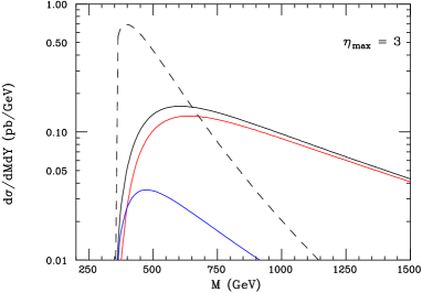
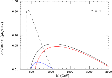
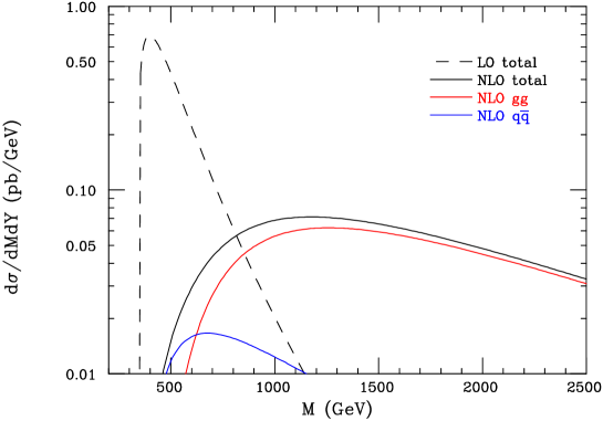
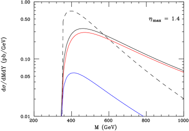
Resummed results corresponding to fig. 1 are shown in fig. 2. We see that the peak of the distribution has moved to much higher mass, beyond 1 TeV. This is due to multiple emission of ISR partons in the evolution of the initial state from the detection scale $Q_{c}$ to the hard subprocess scale $Q$. As the value of $\eta_{\rm max}$ is reduced, the range of evolution becomes smaller, less ISR is emitted, and the peak moves closer to the hard subprocess scale, as illustrated in fig. 3. However, recall that any loss of visible particles produced in the hard subprocess (top decay products in this case) has been neglected here. Such losses will cause the peak to fall below the hard subprocess scale at low values of $\eta_{\rm max}$. In ref. [41] it was found that when $\eta_{\rm max}=1.4$ the peak lies close to threshold for the hard subprocesses studied there, presumably as a result of compensation between ISR and loss of visible decay products.

Figure 2: Resummed distribution of visible mass $M$ in $t\bar{t}$ production at LHC for $\eta_{\rm max}=5$ and $Y=0$.

Figure 3: Resummed distribution of visible mass $M$ in $t\bar{t}$ production at LHC for $Y=0$ and lower values of $\eta_{\rm max}$: colour scheme as in figs.1 and 2.

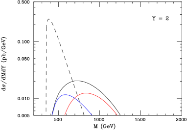
Results for higher values of the visible rapidity $Y$ are shown in fig. 4. The peak moves to lower mass as $Y$ increases, as a consequence of the suppression of high masses by the rapid fall-off of the parton distributions at high $x$.

Figure 4: Resummed distribution of visible mass $M$ in $t\bar{t}$ production at LHC for $\eta_{\rm max}=5$: results at non-zero visible rapidity $Y$.

4 Monte Carlo comparisons

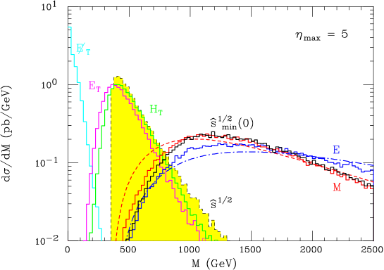
In this section we compare the predictions of the above analytical treatment with Monte Carlo results from HERWIG [43, 44]. Figure 5 shows the Monte Carlo results for various global inclusive observables in $t\bar{t}$ production at the LHC when $\eta_{\rm max}=5$. For the detector simulation we used GETJET [45] with calorimeter cell size $(\Delta\eta,\Delta\phi)=(0.1,0.1)$. To facilitate the study of ISR effects, the simulated underlying event was turned off.

Figure 5: Monte Carlo results for various inclusive observables in $t\bar{t}$ production at LHC. The yellow filled histogram shows the true hard subprocess invariant mass. The dashed red and dot-dashed blue curves show the results of eqs. (56) and (57) , respectively, integrated with respect to $Y$.

As expected, the distributions of variables that involve longitudinal momenta are broadened and shifted relative to those of purely transverse quantities. The distributions of the visible mass $M$ and the new quantity (2) are similar, while the visible energy $E$ has a broader distribution, as it includes the visible momentum.

Comparing the visible mass and energy distributions with the analytical calculations (the dashed red and dot-dashed blue curves, respectively), we find good overall agreement, considering the simplifications made in the latter, viz. the quasi-collinear approximation, no loss of top decay products and no hadronization. In addition, turning off the underlying event in the Monte Carlo does not entirely eliminate contributions from spectator parton fragments at high rapidity.

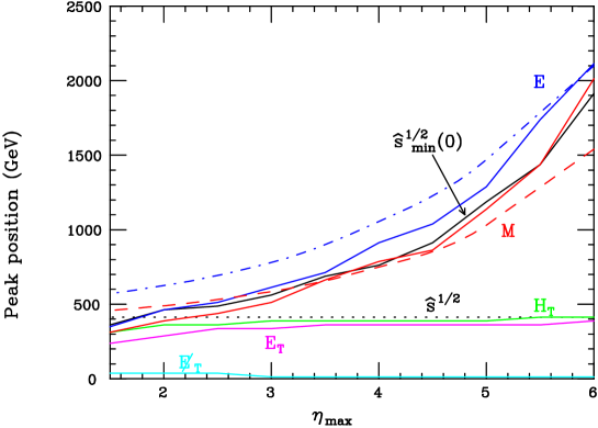
Figure 6: Position of peaks in the distributions of various inclusive observables in $t\bar{t}$ production at LHC, as a function of the maximum visible pseudorapidity $\eta_{\rm max}$. Solid curves: Monte Carlo results. Dashed red and dot-dashed blue curves: $M$ and $E$ peaks from eqs. (56) and (57), respectively. Dotted line: $t\bar{t}$ invariant mass peak.

The motion of the peaks in these distributions as the maximum visible pseudorapidity $\eta_{\rm max}$ is varied is shown in fig. 6. The distributions of the transverse quantities remain remarkably stable, while the peak positions of the other variables rise faster than linearly with increasing $\eta_{\rm max}$. The analytical prediction for the peak position of the visible mass is in good agreement with the Monte Carlo results at intermediate values of $\eta_{\rm max}$ but somewhat higher at low values and lower at high values. This is consistent with the loss of top decay products at low $\eta_{\rm max}$ and the contribution of spectator fragments at high $\eta_{\rm max}$ in the Monte Carlo. The peak position of the visible energy distribution is somewhat overestimated at all but the highest values of $\eta_{\rm max}$. However, as may be seen from fig. 5, the distribution of this quantity is quite flat near the peak, and therefore a small discrepancy between the analytical and Monte Carlo results can give rise to a larger difference in the associated peak positions.

More precise Monte Carlo studies of global inclusive observables like those considered here could be performed using methods that match parton showers to matrix elements for extra jet production; see for example [46, 47, 48] and references therein. We checked that matching to NLO (up to one extra jet) using MC@NLO [49, 50] did not lead to significantly different results.

5 Conclusions

We have derived a simple analytical formula, eq. (56), for the effects of QCD initial state radiation on the invariant mass $M$ and rapidity $Y$ of the visible part of the final state of a hadronic collision, as a function of the pseudorapidity coverage $\eta_{\rm max}$ of an idealized detector. Given the mass distribution of a hard subprocess involving incoming partons $a^{\prime}$ and $b^{\prime}$, a simple convolution with the universal functions $H_{a^{\prime}b^{\prime},ab}$ in eq. (52) provides the quantities $\Sigma_{ab}$ that, when multiplied by the relevant parton distributions, sampled at an $\eta_{\rm max}$-dependent scale, yield the visible mass and energy distributions.

The derivation involved a number of simplifying assumptions and approximations, but was in satisfactory agreement with Monte Carlo results that should in principle be more realistic. The difference between the visible mass $M$ and the new variable (2) is small when $M_{\rm inv}=0$, essentially because of the relative smallness of the missing transverse energy $\not\!\!E_{T}$, manifest in fig. 5.

Many of the approximations made here could be improved if a more precise analysis is needed. The emission of invisible particles in the hard subprocess could be taken into account by replacing the mass distribution of that process by a visible mass distribution, with the invisible component already integrated out. The universal functions $H_{a^{\prime}b^{\prime},ab}$ could be computed to next-to-leading order, as they involve the same quantities that drive the evolution of the parton distribution functions. Together with an NLO calculation of the hard subprocess mass distribution, this would provide a complete NLO description of the visible mass and energy distributions.

Whether such refinements are worthwhile depends on the extent to which observables involving longitudinal momenta are found useful in the exploration of physics beyond the Standard Model. The Monte Carlo results presented in the previous section confirm that transverse quantities are much less sensitive to the effects of ISR. However, at the very least it will be useful to check the consistency of hypotheses about new subprocesses with the distributions discussed here, which do contain independent information about their scales.

References

• [1] I. Hinchliffe, F. E. Paige, M. D. Shapiro, J. Soderqvist and W. Yao, “Precision SUSY measurements at LHC,” Phys. Rev.  D 55, 5520 (1997) [arXiv:hep-ph/9610544].
• [2] F. E. Paige, “Supersymmetry signatures at the CERN LHC,” arXiv:hep-ph/9801254.
• [3] C. G. Lester and D. J. Summers, “Measuring masses of semi-invisibly decaying particles pair produced at hadron colliders,” Phys. Lett.  B 463, 99 (1999) [arXiv:hep-ph/9906349].
• [4] H. Bachacou, I. Hinchliffe and F. E. Paige, “Measurements of masses in SUGRA models at LHC,” Phys. Rev.  D 62, 015009 (2000) [arXiv:hep-ph/9907518].
• [5] I. Hinchliffe and F. E. Paige, “Measurements in SUGRA models with large tan(beta) at LHC,” Phys. Rev.  D 61, 095011 (2000) [arXiv:hep-ph/9907519].
• [6] D. R. Tovey, “Measuring the SUSY mass scale at the LHC,” Phys. Lett.  B 498, 1 (2001) [arXiv:hep-ph/0006276].
• [7] B. C. Allanach, C. G. Lester, M. A. Parker and B. R. Webber, “Measuring sparticle masses in non-universal string inspired models at the LHC,” JHEP 0009, 004 (2000) [arXiv:hep-ph/0007009].
• [8] A. Barr, C. Lester and P. Stephens, “m(T2): The truth behind the glamour,” J. Phys. G 29, 2343 (2003) [arXiv:hep-ph/0304226].
• [9] M. M. Nojiri, G. Polesello and D. R. Tovey, “Proposal for a new reconstruction technique for SUSY processes at the LHC,” arXiv:hep-ph/0312317.
• [10] K. Kawagoe, M. M. Nojiri and G. Polesello, “A new SUSY mass reconstruction method at the CERN LHC,” Phys. Rev.  D 71, 035008 (2005) [arXiv:hep-ph/0410160].
• [11] B. K. Gjelsten, D. J. Miller and P. Osland, “Measurement of SUSY masses via cascade decays for SPS 1a,” JHEP 0412, 003 (2004) [arXiv:hep-ph/0410303].
• [12] B. K. Gjelsten, D. J. Miller and P. Osland, “Measurement of the gluino mass via cascade decays for SPS 1a,” JHEP 0506, 015 (2005) [arXiv:hep-ph/0501033].
• [13] D. J. Miller, P. Osland and A. R. Raklev, “Invariant mass distributions in cascade decays,” JHEP 0603, 034 (2006) [arXiv:hep-ph/0510356].
• [14] C. G. Lester, “Constrained invariant mass distributions in cascade decays: The shape of the ’m(qll)-threshold’ and similar distributions,” Phys. Lett.  B 655, 39 (2007) [arXiv:hep-ph/0603171].
• [15] B. K. Gjelsten, D. J. Miller, P. Osland and A. R. Raklev, “Mass determination in cascade decays using shape formulas,” AIP Conf. Proc.  903, 257 (2007) [arXiv:hep-ph/0611259].
• [16] S. Matsumoto, M. M. Nojiri and D. Nomura, “Hunting for the top partner in the littlest Higgs model with T-parity at the LHC,” Phys. Rev.  D 75, 055006 (2007) [arXiv:hep-ph/0612249].
• [17] H. C. Cheng, J. F. Gunion, Z. Han, G. Marandella and B. McElrath, “Mass Determination in SUSY-like Events with Missing Energy,” JHEP 0712, 076 (2007) [arXiv:0707.0030 [hep-ph]].
• [18] C. Lester and A. Barr, “MTGEN : Mass scale measurements in pair-production at colliders,” JHEP 0712, 102 (2007) [arXiv:0708.1028 [hep-ph]].
• [19] W. S. Cho, K. Choi, Y. G. Kim and C. B. Park, “Gluino Stransverse Mass,” Phys. Rev. Lett.  100, 171801 (2008) [arXiv:0709.0288 [hep-ph]].
• [20] B. Gripaios, “Transverse Observables and Mass Determination at Hadron Colliders,” JHEP 0802, 053 (2008) [arXiv:0709.2740 [hep-ph]].
• [21] A. J. Barr, B. Gripaios and C. G. Lester, “Weighing Wimps with Kinks at Colliders: Invisible Particle Mass Measurements from Endpoints,” JHEP 0802, 014 (2008) [arXiv:0711.4008 [hep-ph]].
• [22] W. S. Cho, K. Choi, Y. G. Kim and C. B. Park, “Measuring superparticle masses at hadron collider using the transverse mass kink,” JHEP 0802, 035 (2008) [arXiv:0711.4526 [hep-ph]].
• [23] G. G. Ross and M. Serna, “Mass Determination of New States at Hadron Colliders,” Phys. Lett.  B 665, 212 (2008) [arXiv:0712.0943 [hep-ph]].
• [24] M. M. Nojiri, G. Polesello and D. R. Tovey, “A hybrid method for determining SUSY particle masses at the LHC with fully identified cascade decays,” JHEP 0805, 014 (2008) [arXiv:0712.2718 [hep-ph]].
• [25] P. Huang, N. Kersting and H. H. Yang, “Hidden Thresholds: A Technique for Reconstructing New Physics Masses at Hadron Colliders,” arXiv:0802.0022 [hep-ph].
• [26] M. M. Nojiri, Y. Shimizu, S. Okada and K. Kawagoe, “Inclusive transverse mass analysis for squark and gluino mass determination,” JHEP 0806, 035 (2008) [arXiv:0802.2412 [hep-ph]].
• [27] D. R. Tovey, “On measuring the masses of pair-produced semi-invisibly decaying particles at hadron colliders,” JHEP 0804, 034 (2008) [arXiv:0802.2879 [hep-ph]].
• [28] M. M. Nojiri and M. Takeuchi, “Study of the top reconstruction in top-partner events at the LHC,” arXiv:0802.4142 [hep-ph].
• [29] H. C. Cheng, D. Engelhardt, J. F. Gunion, Z. Han and B. McElrath, “Accurate Mass Determinations in Decay Chains with Missing Energy,” Phys. Rev. Lett.  100, 252001 (2008) [arXiv:0802.4290 [hep-ph]].
• [30] W. S. Cho, K. Choi, Y. G. Kim and C. B. Park, “Measuring the top quark mass with mT2subscript𝑚𝑇2m_{T2} at the LHC,” Phys. Rev.  D 78, 034019 (2008) [arXiv:0804.2185 [hep-ph]].
• [31] M. Serna, “A short comparison between mT2subscript𝑚𝑇2m_{T2} and mCTsubscript𝑚𝐶𝑇m_{CT},” JHEP 0806, 004 (2008) [arXiv:0804.3344 [hep-ph]].
• [32] M. Bisset, R. Lu and N. Kersting, “Improving SUSY Spectrum Determinations at the LHC with Wedgebox and Hidden Threshold Techniques,” arXiv:0806.2492 [hep-ph].
• [33] A. J. Barr, G. G. Ross and M. Serna, “The Precision Determination of Invisible-Particle Masses at the LHC,” arXiv:0806.3224 [hep-ph].
• [34] N. Kersting, “On Measuring Split-SUSY Gaugino Masses at the LHC,” arXiv:0806.4238 [hep-ph].
• [35] M. M. Nojiri, K. Sakurai, Y. Shimizu and M. Takeuchi, “Handling jets + missing ETsubscript𝐸𝑇E_{T} channel using inclusive mT2,” arXiv:0808.1094 [hep-ph].
• [36] J. Alwall, M. P. Le, M. Lisanti and J. G. Wacker, “Model-Independent Jets plus Missing Energy Searches,” arXiv:0809.3264 [hep-ph].
• [37] W. S. Cho, K. Choi, Y. G. Kim and C. B. Park, “MT2subscript𝑀𝑇2M_{T2}-assisted on-shell reconstruction of missing momenta and its application to spin measurement at the LHC,” arXiv:0810.4853 [hep-ph].
• [38] H. C. Cheng and Z. Han, “Minimal Kinematic Constraints and MT2,” arXiv:0810.5178 [hep-ph].
• [39] M. Burns, K. Kong, K. T. Matchev and M. Park, “Using Subsystem MT2 for Complete Mass Determinations in Decay Chains with Missing Energy at Hadron Colliders,” arXiv:0810.5576 [hep-ph].
• [40] A. J. Barr, A. Pinder and M. Serna, “Precision Determination of Invisible-Particle Masses at the CERN LHC: II,” arXiv:0811.2138 [hep-ph].
• [41] P. Konar, K. Kong and K. T. Matchev, “sminsubscript𝑠min\sqrt{s}_{\rm min}: a global inclusive variable for determining the mass scale of new physics in events with missing energy at hadron colliders,” arXiv:0812.1042 [hep-ph].
• [42] A. D. Martin, W. J. Stirling, R. S. Thorne and G. Watt, “Parton distributions for the LHC,” arXiv:0901.0002 [hep-ph].
• [43] G. Corcella et al., “HERWIG 6.5: an event generator for Hadron Emission Reactions With Interfering Gluons (including supersymmetric processes),” JHEP 0101 (2001) 010 [arXiv:hep-ph/0011363].
• [44] G. Corcella et al., “HERWIG 6.5 release note,” arXiv:hep-ph/0210213.
• [45] F. Paige, private communication; F. Paige and S. Protopopescu, “ISAJET 5.02: a Monte Carlo event generator for pp𝑝𝑝pp and p¯p¯𝑝𝑝\bar{p}p interactions,” in Supercollider Physics, ed. D. Soper (World Scientific, Singapore, 1986), p. 41.
• [46] M. L. Mangano, M. Moretti, F. Piccinini and M. Treccani, “Matching matrix elements and shower evolution for top-quark production in hadronic collisions,” JHEP 0701 (2007) 013 [arXiv:hep-ph/0611129].
• [47] J. Alwall, S. de Visscher and F. Maltoni, “QCD radiation in the production of heavy colored particles at the LHC,”’ JHEP 0902 (2009) 017 [arXiv:0810.5350 [hep-ph]].
• [48] S. Hoeche, F. Krauss, S. Schumann and F. Siegert, “QCD matrix elements and truncated showers,” JHEP 0905 (2009) 053 [arXiv:0903.1219 [hep-ph]].
• [49] S. Frixione and B. R. Webber, “Matching NLO QCD computations and parton shower simulations,” JHEP 0206 (2002) 029 [arXiv:hep-ph/0204244].
• [50] S. Frixione, P. Nason and B. R. Webber, “Matching NLO QCD and parton showers in heavy flavour production,” JHEP 0308 (2003) 007 [arXiv:hep-ph/0305252].