Negative-continuum dielectronic recombination
into excited states of highly–charged ions

Abstract

The recombination of a free electron into a bound state of bare, heavy nucleus under simultaneous production of bound–electron—free–positron pair is studied within the framework of relativistic first–order perturbation theory. This process, denoted as “negative–continuum dielectronic recombination” leads to a formation of not only the ground but also the singly– and doubly–excited states of the residual helium–like ion. The contributions from such an excited–state capture to the total as well as angle–differential cross-sections are studied in detail. Calculations are performed for the recombination of (initially) bare uranium U⁹²⁺ ions and for a wide range of collision energies. From these calculations, we find almost 75 % enhancement of the total recombination probability if the excited ionic states are taken into account.

I Introduction

Owing to the recent advances in heavy–ion accelerators and ion storage rings, the electron–positron pair creation in ion–atom (or ion–ion) collisions attracts much of today’s interest both in experiment and theory Eichler and Meyerhof (1995); Eichler (2005); Baur et al. (2007). The investigation of this process is of great importance not only for a better understanding of the physics of extremely strong electromagnetic fields but also for the development of novel collider facilities Baltz et al. (1996); Bruce et al. (2007). A large number of studies are focused, therefore, on the bound–free pair production in which electron is created in an atomic (ionic) shell under a simultaneous emission of a free positron. Experimentally, such a pair production is usually observed in relativistic collisions of highly–charged ions with medium– and high–$Z$ atomic targets Belkacem et al. (1993); Vane et al. (1997); Belkacem et al. (1998). Special attention in these experimental studies is paid to the total (pair creation) cross-sections and to their dependence on both the collision energy and the nuclear charge of both the projectile and the target. Theoretical analysis of the total cross-sections is not a simple task since it usually requires the solution of the two–center time–dependent Dirac equation. Even though a number of approaches, such as the coupled–channel methods Reinhardt et al. (1978); Müller-Nehler and Soff (1994); Eichler and Meyerhof (1995); Eichler (2005) and the lattice numerical solutions Ionescu and Belkacem (1999); Busic et al. (2004), have been developed to deal with the two–center Dirac problem, they result in very demanding and time–consuming calculations.

Apart from the energetic collisions of high–$Z$ projectiles with heavy atomic targets, an alternative and very promising route has been offered recently to investigate the bound–electron—free–positron production. In this process a free incoming electron is captured into a bound state of heavy, highly–charged ion and the released energy is converted into an electron–positron pair Artemyev et al. (2003). Due to the schematic similarity to the usual dielectronic recombination of few–electron ions, this process has been denoted as negative continuum dielectronic recombination (NCDR). It is important to outline, however, that in contrast to dielectronic recombination, the electron to be “excited” in NCDR is not initially bound to an ion but an electron from the negative continuum. Therefore, negative continuum dielectronic recombination of a free electron with an initially bare nucleus of charge $Z$ results in the production of a helium–like ion and a free outgoing positron:

$$X^{Z+}+e^{-}\,\rightarrow\,X^{(Z-2)+}+e^{+}\,.$$ (1)

Of course, this reaction has a threshold and becomes possible only if the energy of incoming electron in the center of mass rest frame is larger than the sum of the positron rest energy and the energy of the residual helium–like ion.

Unlike the other mechanisms of pair creation, the NCDR involves only one–center Dirac problem which significantly simplifies its theoretical analysis. In Ref. Artemyev et al. (2003), for example, the first–order perturbation approach has been developed to study the properties of the emitted positron and the total recombination probabilities. Within this approach, based on relativistic Dirac’s theory, detailed calculations have been carried out for the cross-sections of the NCDR into the ground $(1s)^{2}$ state of (initially) bare led Pb⁸²⁺ and uranium U⁹²⁺ ions. These calculations have indicated that the ground–state recombination cross-sections do not exceed the value of 30 $\mu$bar. This makes, experimental study of the NCDR process rather difficult. It was argued, however, that a significant enhancement of the NCDR probability can be expected due to electron transfer into excited states of finally helium–like ions. Together with the unique signature of ionic charge change by two units accompanied by a simultaneous positron emission [cf. Eq. (1)], such an enhancement shall render the NCDR process observable with the advent of the new generation of heavy–ion storage rings with high beam intensities such as, for example, at the future Facility for Antiproton and Ion Research (FAIR) at Darmstadt GSI (2001).

Despite its impact on the planned FAIR experiments, the influence of the excited–state recombination on the total NCDR probability has not been studied in detail until now. A first step towards such a study was performed by us in Ref. Artemyev et al. (2005) where the electron transfer into some low–lying bound states of high–$Z$, bare ions has been investigated. Relativistic calculations performed in Ref. Artemyev et al. (2005) have confirmed the significant role of excited–state NCDR but have faced us to the necessity of a more systematic analysis.

In this contribution, we apply here the first–order perturbation theory based on the relativistic Dirac’s equation to explore a negative continuum dielectronic recombination of a free electron into singly– and doubly–excited states of (initially) bare, highly–charged ions. Special emphasis in our present study is placed on the contributions which come from the excited–state capture to both, the total and the angle–differential NCDR cross sections. The basic expressions for these cross-sections, as obtained within the framework of the independent particle model (IPM) for the description of the (final) two–electron states, are discussed in Section II. In particular, it is argued that any analysis of the NCDR properties can be traced back to the transition amplitudes which describe the interelectronic interaction in the capture process. In Section III, the evaluation of these matrix elements is briefly outlined. Results of our fully relativistic calculations are presented then in Section IV for the initially bare uranium ions U⁹²⁺ and for a wide range of collision energies. The calculations have been carried out for the NCDR into all singly–excited $(1snl_{j})_{J}$ with $n\leq 4$ and doubly–excited $(2s2l_{j})_{J}$ states. In order to take into account even higher–lying states, an extrapolation of our results has been performed to larger principal quantum numbers $n$. By making use of such an extrapolation procedure we have found that the recombination into excited ionic states may enhance the total cross-section by about 75 % when compared to the ground–state NCDR. A brief summary of this important finding and its implication for future experiments is finally given in Section V.

Relativistic units ($\hbar=m_{e}=c=1$) are used throughout the paper. In the following, moreover, electron energies are always defined as including the electron rest mass.

II Theory

Not much has to be said about the basic formalism for studying the negative continuum dielectronic recombination of high–$Z$ bare ions. Recently, this formalism, based on the quantum electrodynamical approach, has been discussed by us in Refs. Artemyev et al. (2003, 2005). In particular, we argued that to zeroth order of perturbation theory, NCDR is given by the diagram shown in Fig. 1. In this diagram, ${p}_{i}$ is the asymptotic momentum of the incoming electron and $a$ and $b$ denote the quantum states of the (finally) bound electrons. Moreover, according to the standard procedure Bjorken and Drell (1965); Itzykson and Bernard Zuber (1980), the outgoing positron with four-momentum $p_{f}$ is described as an incoming electron with four-momentum $-p_{f}$.

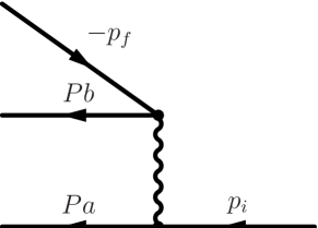
Figure 1: Feynman diagram for the negative-continuum dielectronic recombination. $a$ and $b$ are the bound one-electron states and $P$ is the permutation operator.

Evaluation of the diagram depicted in Fig. 1 requires the knowledge of the (two–electron) wavefunction of the final ionic state. Since our analysis of the NCDR process is restricted to heavy ions for which the electron–electron interaction effects are usually small, it is convenient to describe this wavefunction within the framework of the independent particle model (IPM). That is, the wavefunction of the final helium–like ion with the well–defined angular momentum $J$ and its projection $M$ is approximated by means of Slater determinants built from hydrogenic orbitals:

$$\Psi^{bound}_{JM}({\bf r}_{1},{\bf r}_{2}) = N\sum_{m_{a},m_{b}}C_{j_{a}m_{a},\,j_{b}m_{b}}^{JM}$$

$$\times\left|\begin{array}[]{ll}\psi_{n_{a}\kappa_{a}m_{a}}({\bf r}_{1})&\psi_{n_{b}\kappa_{b}m_{b}}({\bf r}_{1})\\ \psi_{n_{a}\kappa_{a}m_{a}}({\bf r}_{2})&\psi_{n_{b}\kappa_{b}m_{b}}({\bf r}_{2})\end{array}\right|$$

$$= N\sum_{m_{a},m_{b}}C_{j_{a}m_{a},\,j_{b}m_{b}}^{JM}\sum_{P}(-1)^{P}$$

$$\times \psi_{n_{Pa}\kappa_{Pa}m_{Pa}}({\bf r}_{1})\psi_{n_{Pb}\kappa_{Pb}m_{Pb}}({\bf r}_{2})\,.$$ (5)

Here, $\psi_{n_{a}\kappa_{a}m_{a}}(\bm{r})$ and $\psi_{n_{b}\kappa_{b}m_{b}}(\bm{r})$ are the well–known solutions of the Dirac’s equation for a bound electron, $C_{j_{a}m_{a},\,j_{b}m_{b}}^{JM}$ is the Clebsch–Gordan coefficient, $P$ is the permutation operator, $(-1)^{P}$ is the permutation parity and $N$ is the normalization factor. As usual, this factor is $N=1/2$ for $n_{a}=n_{b}$, $\kappa_{a}=\kappa_{b}$ and $N=1/\sqrt{2}$ otherwise.

By making use of the final state wavefunction (II) we are able to evaluate the Feynman diagram from Fig. 1 and, hence, to find the differential (in positron emission angle) NCDR cross–section in the center of mass rest–frame:

$$\frac{d\sigma}{d\Omega_{f}}(n_{a}\kappa_{a},n_{b}\kappa_{b};J) = \frac{16\pi^{4}N^{2}}{v_{i}}{\bf p}_{f}^{2}$$

$$\times\sum_{M}\sum_{m_{a},\,m_{b}}\sum_{m_{i},\,m_{f}}\Big{|}\sum_{P}(-1)^{P}C^{J\,M}_{j_{a}m_{a},\,j_{b}m_{b}}$$

$$\times\left\langle PaPb\left|I(\varepsilon_{i}-\varepsilon_{Pa})\right|{p}_{i},m_{i},-{p}_{f},m_{f}\right\rangle\Big{|}^{2}\,,$$

where we assume that the incident electron is unpolarized and the spin states of the residual ion and emitted positron remain unobserved. In Eq. (II), moreover, for the sake of shortness we denote $|ab\rangle\equiv|n_{a}\kappa_{a}m_{a},n_{b}\kappa_{b}m_{b}\rangle$, $\varepsilon_{i}$ and $\varepsilon_{a,b}$ are the one–electron Dirac energies of the incoming and bound electrons, respectively, and $I(\omega)$ is the electron–electron interaction operator. In Coulomb and Feynman gauges this operator reads:

$$I_{C}(\omega) = \alpha\left(\frac{1}{r_{12}}-({\mbox{\boldmath$\alpha$}}_{1}\cdot{\mbox{\boldmath$\alpha$}}_{2})\frac{\exp(i|\omega|r_{12})}{r_{12}}\right.$$

$$+ \left.\Big{[}({\mbox{\boldmath$\alpha$}}_{1}\cdot{\mbox{\boldmath$\nabla$}}_{1}),\Big{[}({\mbox{\boldmath$\alpha$}}_{2}\cdot{\mbox{\boldmath$\nabla$}}_{2}),\frac{\exp(i|\omega|r_{12})-1}{\omega^{2}r_{12}}\Big{]}\Big{]}\right)\,,$$

$$I_{F}(\omega) = \alpha(1-{\mbox{\boldmath$\alpha$}}_{1}\cdot{\mbox{\boldmath$\alpha$}}_{2})\frac{\exp(i|\omega|r_{12})}{r_{12}}\,,$$ (8)

where $r_{12}=|{\bf r}_{1}-{\bf r}_{2}|$ and ${\bm{\alpha}}_{k}$ denotes the vector of Dirac matrices for the $k$th electron. Below, we employ the Feynman gauge to calculate the NCDR cross-sections. It is obvious, however, that the results obtained are gauge invariant since both the free– and bound–state wavefunctions in Eq. (II) are exact solutions of the Dirac equation.

The transition matrix element in the last line of Eq. (II) contains the wavefunctions of incoming electron $\left|{p}_{i}m_{i}\right\rangle$ and outgoing positron $\left|-{p}_{f}m_{f}\right\rangle$ with the well defined asymptotic momenta. For the further evaluation of the NCDR differential cross-section, it is therefore necessary to decompose these continuum waves into partial waves in order to apply the standard techniques for the theory of angular momentum. As discussed previously, however, special care has to be taken about the choice of the quantization axis since this directly influences the particular form of the partial wave decomposition. Using, for example, the incoming electron momentum ${p}_{i}$ as the quantization axis ($z$–axis), the full expansion of the continuum electron wave function is given by Eichler and Meyerhof (1995); Rose (1961):

$$|{p}_{i}m_{i}\rangle = \frac{1}{\sqrt{4\pi}}\frac{1}{\sqrt{\varepsilon_{i}|{\bf p}_{i}|}}\sum_{\kappa}i^{l}\exp(i\Delta_{\kappa})$$ (9)

$$\times\sqrt{2l+1}C^{j\,m_{i}}_{l\,0,\,(1/2)\,m_{i}}\left|\varepsilon_{i},\kappa,m_{i}\right\rangle\,,$$

where the summation runs over Dirac’s angular momentum quantum number $\kappa=\pm(j+1/2)$ for $l=j\pm 1/2$ with $l$ representing the parity of the partial waves $\left|\varepsilon_{i},\kappa,m_{i}\right\rangle$. In expansion (9), moreover, $\Delta_{\kappa}$ is the Coulomb phase shift and the partial waves

$$\langle{\bf r}|\varepsilon_{i},\kappa,m_{i}\rangle=\left(\begin{array}[]{c}g_{\varepsilon_{i},\kappa}(r)\Omega_{\kappa m_{i}}(\hat{\bf r})\\ if_{\varepsilon_{i},\kappa}(r)\Omega_{-\kappa m_{i}}(\hat{\bf r})\end{array}\right)\,,$$ (12)

decompose in a standard way into a radial and an angular part and, thus, help to carry out the integration over all angles in the NCDR cross-section (II) analytically.

In contrast to the incoming electron, the outgoing positron does not necessarily move along the $z$–axis. In this case it is rather convenient to retain the axis of spin quantization in the direction of $z$–axis and just rotate the space part of the wavefunction Eichler and Meyerhof (1995):

$$|-{p}_{f},m_{f}\rangle = \frac{1}{\sqrt{\varepsilon_{f}|{\bf p}_{f}|}}\sum_{\kappa,M_{f}}i^{l^{\prime}}\exp(i\Delta_{\kappa})$$ (13)

$$\times C^{j\,M_{f}}_{l^{\prime}\,m_{l^{\prime}},\,(1/2)\,m_{f}}Y^{*}_{l^{\prime}m_{l^{\prime}}}(-\hat{p}_{f})$$

$$\times|-\varepsilon_{f},\kappa,M_{f}\rangle\,.$$

Indeed, the value of $m_{f}$ in this expansion does not have any physical meaning since for the relativistic continuum electron (positron) the spin projection has a sharp value only in the direction of propagation (so called helicity). However, since in Eq. (II) we perform summation over all possible spin states of the outgoing positron the use of expansion (13) is well justified.

By inserting now partial wave expansions (9) and (13) into Eq. (II), we finally can write the differential NCDR cross-section as:

$$\frac{d\sigma}{d\Omega_{f}}(n_{a}\kappa_{a},n_{b}\kappa_{b};J) = \frac{4\pi^{3}|{\bf p}_{f}|N^{2}}{\varepsilon_{f}{\bf p}^{2}_{i}}$$

$$\times\sum_{M}\sum_{m_{a}m_{b}}\sum_{m_{i},m_{f}}\Big{|}\sum_{P,\kappa_{i},\kappa_{f},M_{f}}(-1)^{P}$$

$$\times C^{J\,M}_{j_{a}m_{a},\,j_{b}m_{b}}\;i^{l_{i}+l_{f}^{\prime}}\exp(i\Delta_{\kappa_{i}}+i\Delta_{\kappa_{f}})\sqrt{2l_{i}+1}$$

$$\times C^{j_{i}\,m_{i}}_{l_{i}\,0,\,(1/2)\,m_{i}}C^{j_{f}\,M_{f}}_{l_{f}^{\prime}\,m_{l_{f}^{\prime}},\,(1/2)\,m_{f}}Y_{l_{f}^{\prime},m_{l_{f}^{\prime}}}^{*}(-\hat{\bf p}_{f})$$

$$\times\langle PaPb|I(\varepsilon_{i}-\varepsilon_{Pa})|(\varepsilon_{i},\kappa_{i},m_{i})(-\varepsilon_{f},\kappa_{f},M_{f})\rangle\Big{|}^{2}\,.$$

Within the framework of independent particle model this equation is still exact and allows to calculate the cross-section for the negative continuum dielectronic recombination into any possible final configuration of the helium–like ion. In the next Section, for example, we make use of Eq. (II) to investigate electron capture into singly– as well as doubly–excited states of U⁹⁰⁺ ions.

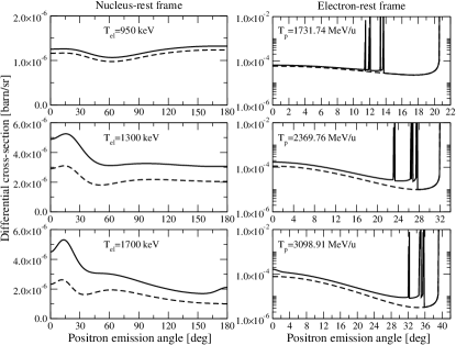
Figure 2: Differential cross-section in the emitted positron angle for the NCDR into $(1s)^{2}$ state (dashed line) and sum of the cross-sections into all possible $(1snl_{j})$ with $n\leq 4$ and $(2s2l_{j})$ states (solid line).

III Computation

As seen from Eq. (II), any further analysis of the NCDR angle–differential cross-sections can be traced back to the transition amplitude:

$$M(a,b)$$

$$=\left\langle n_{a}\kappa_{a}m_{a},n_{b}\kappa_{b}m_{b}\left|I(\varepsilon_{i}-\varepsilon_{a})\right|(\varepsilon_{i},\kappa_{i},m_{i})(-\varepsilon_{f},\kappa_{f},M_{f})\right\rangle$$

which describes the interelectronic interaction during the capture process. In the computations below, we make use of the single–particle Dirac’s wavefunctions modified for the finite nuclear size in order to evaluate such an amplitude. Similar to our previous work Artemyev et al. (2003), the radial components of these wavefunctions have been calculated with the help of the RADIAL package Salvat et al. (1995). This package can be applied for computation of both bound and continuum solutions of the Dirac equation, but only for positive energies. In order to find negative–continuum solutions, we used the fact that the large $g_{-\varepsilon,-\kappa}^{(e^{-})}$ and the small $f_{-\varepsilon,-\kappa}^{(e^{-})}$ radial components of the electron wave function can be expressed in terms of the positron function components as $g_{-\varepsilon,-\kappa}^{(e^{-})}(r)=f_{\varepsilon,\kappa}^{(e^{+})}(r)$, $f_{-\varepsilon,-\kappa}^{(e^{-})}(r)=g_{\varepsilon,\kappa}^{(e^{+})}(r)$ Rose (1961).

By making use of the standard two–component representation (12) of the electron (and positron) wavefunctions as well as the multipole expansion of the interelectronic interaction operator (II), we were able to separate NCDR transition amplitude (III) into the radial and the spin–orbital parts. While the latter can be evaluated analytically using the calculus of the irreducible tensor operators Balashov et al. (2000), the radial integrations have been accomplished numerically with the help of Gauss–Legendre quadratures. To perform this two-dimensional integration we used the standard technique, elaborated for the calculation of such integrals in the case when all four wave function describe bound electrons (see e.g. Ref. Johnson et al. (1988)). However, for relativistic ion–atom collisions such an integration is not a simple task due to the rapid oscillations of the Dirac continuum wavefunctions. In order to overcome this problem we had to use much denser grid of integration knots, than in the case of bound wave functions. Most seriously these oscillations affect NCDR calculations for the highly–excited ionic states which have a significant overlap with the continuum spectrum. In order to achieve a required accuracy of 0.01 % in the computation of radial integrals for these states, we have used few hundreds integration grid points in the Gauss–Legendre procedure. Stability of our numerical results with respect to the exact number and position of radial knots has been proved in series of calculations.

Apart from the influence of the particular integration (Gauss–Legendre) scheme, the role of nuclear–size effect in the numerical evaluation of the NCDR cross sections has been also verified. By making use of the RADIAL package, calculations have been performed not only for the (finite–size) nucleus with root-mean-square radius of 5.86 fm but also for the point–like nucleus. Nuclear–size effect, found from this calculations does not exceed the level of 0.1% which is well below experimental accuracy of the planned NCDR experiments.

IV Results and discussion

After a brief discussion of the theoretical background and the main computational procedures we are ready now to focus on the question of how the electron capture into (highly) excited ionic states affects the total NCDR cross-section $\sigma_{tot}$. We define such a cross-section as a sum over all partial cross-sections describing recombination into possible particular states of the (finally) helium–like projectile:

$$\sigma_{tot} = \sum\limits_{n_{a}\kappa_{a},n_{b}\kappa_{b};J}\sigma(n_{a}\kappa_{a},n_{b}\kappa_{b};J)\,,$$ (16)

where, in turn, $\sigma(n_{a}\kappa_{a},n_{b}\kappa_{b},J)$ is obtained upon integration of Eq. (II) over the positron emission angle:

$$\sigma(n_{a}\kappa_{a},n_{b}\kappa_{b},J)=\int{\frac{d\sigma}{d\Omega_{f}}(n_{a}\kappa_{a},n_{b}\kappa_{b};J)\,{\rm d}\Omega_{f}}\,.$$ (17)

Most naturally, this angular integration can be performed analytically by using the explicit form of the differential cross section (II) and the orthogonality properties of the spherical harmonics.

Before presenting results of our calculations for the total NCDR cross sections, first we would like to discuss the influence of the excited–state recombination on the emission pattern of positrons. In Fig. 2, we display the differential cross sections (II) as a function of positron emission angle for the recombination into helium–like U⁹⁰⁺ ions. In the left column of the figure results of our fully relativistic calculations are presented in the rest frame of the ion which—to zeroth order in $m_{el}/M_{ion}$—coincides with the center of mass rest–frame. Within this frame we have studied positron emission patterns for three kinetic energies of incoming electron: 950 keV (upper panel), 1300 keV (middle panel) and 1700 keV (lower panel). For all three energies we present not only the $K$–shell capture cross section (dashed line) but also the sum of the partial (differential) cross-sections for the NCDR into all singly excited states $(1s\,nl_{j})_{J}$ with $n\leq 4$ and doubly–excited states $(2s\,2l_{j})_{J}$. As seen from Fig. 2, while the capture into these states almost does not affect the NCDR cross-section at the near–threshold energy of $T_{el}$ = 950 keV, it results in a significant enhancement of positron emission for higher electron velocities. For the collision energy of $T_{el}=1700$ keV, for example, the NCDR cross-section increases by about factor of two if the recombination into excited ionic states is taken into account.

Until now we have discussed the NCDR differential cross-sections only in the rest frame of the ion. While the theoretical analysis of the electron recombination process is easier to be performed in such a projectile frame, the forthcoming experimental results on the positron emission most likely will be obtained in the electron rest–frame (laboratory frame). In the following, therefore, we shall apply the Lorenz transformation in order to find the cross-section (II) in the laboratory frame. As it was already discussed in Refs. Artemyev et al. (2003); Eichler and Meyerhof (1995); Dedrick (1962), such a transformation predicts that positron emission in the laboratory frame is possible only within the forward hemisphere and that the maximal emission angle is given by:

$$\sin(\theta_{\rm max})=\frac{\beta_{p}\gamma_{p}}{\beta_{n}\gamma_{n}}\,.$$ (18)

Here, $\gamma=1/\sqrt{1-\beta^{2}}$ is the relativistic Lorenz factor and $\beta$ denotes the velocity (in units of the speed of light). Moreover, the values with sub–index ${}^{\prime\prime}p^{\prime\prime}$ correspond to the positron’s speed and Lorenz factor in the nucleus–rest frame while ones with sub–index ${}^{\prime\prime}n^{\prime\prime}$ to the nucleus in the laboratory frame.

Table 1: The total cross-section of NCDR into the $(1snl_{j})$, and $(2s2l_{j})$ states of U⁹⁰⁺ (initial charge state 92+). Units are keV for the kinetic energy of the electron, $\mu$barn for the cross sections.

$T_{el}$	950	1300	1700
$(1s)^{2}$	13.8	26.7	20.0
$(1s2s)$	6.82$\times 10^{-1}$	7.47	5.91
$(1s2p)$	2.62$\times 10^{-1}$	2.87	2.41
$(1s3s)$	9.49$\times 10^{-2}$	2.12	1.73
$(1s3p)$	4.02$\times 10^{-2}$	9.58$\times 10^{-1}$	8.18$\times 10^{-1}$
$(1s3d)$	7.80$\times 10^{-4}$	1.37$\times 10^{-2}$	1.88$\times 10^{-2}$
$(1s4s)$	2.38$\times 10^{-2}$	8.40$\times 10^{-1}$	6.95$\times 10^{-1}$
$(1s4p)$	1.22$\times 10^{-2}$	4.16$\times 10^{-1}$	3.54$\times 10^{-1}$
$(1s4d)$	3.33$\times 10^{-4}$	8.89$\times 10^{-3}$	7.41$\times 10^{-3}$
$(1s4f)$	2.61$\times 10^{-5}$	2.97$\times 10^{-4}$	1.01$\times 10^{-3}$
$(2s)^{2}$		4.69$\times 10^{-1}$	4.41$\times 10^{-1}$
$(2s2p)$		3.38$\times 10^{-1}$	3.37$\times 10^{-1}$
$\Sigma$	14.9	42.2	32.7
Extrapolated	14.9	44.3(7)	34.5(9)

Existence of the maximal emission angle (18) leads to the fact that the differential NCDR cross-section (II) calculated in the laboratory frame becomes infinite when $\theta_{f}=\theta_{\rm max}$ [cf. Ref. Artemyev et al. (2003) for further details]. This singularity appears, however, only for the “model” calculations with monochromatic ions and electrons. If one considers, in contrast, some velocity distribution of the particles either in electron target or/and in ion beam such a singularity transforms into a resonant peak. Theoretical investigation of the peak structures in the NCDR cross-section is currently underway and will be reported in a upcoming publication.

It immediately follows from Eq. (18) and the energy conservation condition that the maximal positron emission angle $\theta_{\rm max}$ and, hence, the (position of) singularity in the recombination cross-section, depends on the energy of the final helium–like state. This can be observed in the right column of Fig. 2 where the NCDR cross-section is displayed in the laboratory frame as a function of positron emission angle. As seen from the figure, the positrons emitted in the $K$–shell NCDR have the largest angle $\theta_{\rm max}$. This angle is drastically reduced, however, for the electron capture into (weaker bound) excited ionic states. Such an energy– and, hence, state–dependence of the NCDR differential cross-section provides a unique possibility to separate experimentally the positrons which are emitted in course of the ground– as well as excited–state electron recombination. Moreover, the existence of the maximal angle $\theta_{\rm max}$ may allow one to distinguish NCDR from the other—competitive—processes which also result in positron emission. Obviously, this becomes possible if one starts to detect the outgoing positrons at the polar angles larger then the maximal one for the NCDR into the ground state.

Up to the present we have discussed the angle–differential NCDR cross-sections both in the projectile (ion–rest) and in the laboratory (electron–rest) frames. Integration of these cross sections over the positron emission angle and summation over all configurations (see Eqs. (16)–(17)) will yield the total NCDR cross-section. In contrast to the angle–differential ones, this cross-section does not depend on the particular frame [cf. Ref. Artemyev et al. (2003) for further discussion]. Hence, one can perform the integration over the positron emission angles in both the ion– and the electron–rest frames. Below, for example, the total cross-sections are calculated within the projectile frame which is more preferable from the computational viewpoint because of the absence of the singularities in the positron angular distribution.

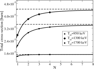
Figure 3: The convergence of the NCDR cross-sections $\sigma_{N}$ (cf. Eq. (19)) with increasing of $N$ and it’s extrapolation. The symbols are numerical results, the solid lines represent their interpolation by the third degree polynomials in inverse powers of $N$, and the dashed lines are the limits of these polynomials at $N\rightarrow\infty$.

As seen from Eq. (16), the computation of the total NCDR cross-section $\sigma_{\rm tot}$ requires first a knowledge of the partial cross-sections $\sigma(n_{a}\kappa_{a},n_{b}\kappa_{b},J)$ describing the electron recombination into the particular two–electron states $\left|n_{a}\kappa_{a},n_{b}\kappa_{b};J\right\rangle$. In our present work, for instance, we take into account all singly–excited $(1s\,nl_{j})$ (up to $(1s\,4f_{7/2})$) and doubly–excited $(2s\,2l_{j})$ states of finally helium–like uranium U⁹⁰⁺ ions. The partial cross-sections for the recombination into these states are given in Table 1 for three energies of incoming electron: $T_{kin}=$ 950 keV, 1300 keV and 1700 keV. As seen from the table, the probability of the NCDR process significantly reduces for the highly excited ionic states. For instance, the cross-section of the recombination into the $(1s\,4f_{7/2})_{3,4}$ levels is about four orders of magnitude smaller comparing with the ground–state one $\sigma((1s)^{2})$. Such a behavior of the NCDR probabilities allowed us to apply an extrapolation scheme in order to estimate the contribution from the $(1s\,nl_{j})$ states with $n>4$ to the total cross-section (16). That is, by employing the polynomials in inverse powers of $N$ for fitting the cross–sections

$$\sigma_{N}=\sum_{n=1}^{N}\sum_{ljJ}\sigma(1s\,nl_{j};J)\,,$$ (19)

we were able to find $\sigma_{\rm tot}=\lim_{N\to\infty}\sigma_{N}$. Application of the $(1/N)^{l}$–polynomial fitting seems to be justified since both the (ordinary) electron capture and bound–state pair production cross sections are known to scale roughly as $1/N^{3}$ Eichler and Meyerhof (1995). One may expect, therefore, similar $N$–dependence for the NCDR process which leads to a production of a singly–excited helium–like ions. The extrapolation procedure is illustrated in Fig. 3, where the symbols display our numerical results for $\sigma_{N}$ taken for $N=1...4$, solid lines plot the interpolation polynomials, and dashed lines indicate their limits at $N\to\infty$. In contrast to the singly–excited states, no extrapolation procedure has been applied for the high–$n$ doubly–excited states since their contribution to the total NCDR cross-section (16) was found to be negligible. Instead, we just added partial cross-sections $\sigma(2s\,2l_{j})$ to the results of the extrapolation over $(1s\,nl_{j})$ states.

In order to estimate an accuracy of our extrapolation scheme, we have used first only the levels with $n=$ 1, 2 and 3 in order to find a fitting function. Then we repeated the same procedure but now including cross sections for the recombination into the $(1s\,4l_{j})$ states. The second asymptotic limit was found to be in about 1–2% agreement with the first one.

The total NCDR cross-sections $\sigma_{\rm tot}$ obtained by means of the procedure discussed above are given in the last row of Table 1 together with the estimations of the computational error. These estimations have been derived by comparing the results of the extrapolation procedure performed with the help of the polynomials of different degrees. As seen from the last row of the table, negative continuum dielectronic recombination into excited ionic states results in a significant enhancement of the total cross-section $\sigma_{\rm tot}$ when compared with the ground–state capture (cf. first row of the table). Moreover, the role of the excited states in the NCDR process increases with increasing kinetic energy of the electron. While, for example, the excited–state contribution to the total cross-section (16) does not exceed 8 % for the electron kinetic energy of $T_{\rm el}=$ 950 keV, it increases to almost 75 % for $T_{\rm el}=$ 1700 keV. Such a behavior can be easily explained by the fact that the threshold of the NCDR process depends on the total energy $E_{ab}$ of the (final) two–electron system (II) as:

$$\varepsilon_{ab}^{\rm th} = E_{ab}+mc^{2}\,,$$ (20)

and, hence, increases for excited ionic states. Therefore, since close to threshold the probability of the NCDR is very low due to strong exponential damping of the low-energy positron wave function in the region close to the nucleus, the role of the excited–state recombination becomes more pronounced only for rather high collision energies.

In Table 1 we have presented the total (16) as well as partial (17) NCDR cross-sections for only three energies of incoming electron. In order to study the energy dependence of these cross-sections in more detail we plot them in Fig. 4 as a function of $T_{el}$. Similar to before, the dashed curve in the figure represents the partial cross–section $\sigma((1s)^{2})$ of the NCDR into the ground state. Next four curves are obtained by adding to $\sigma((1s)^{2})$ the capture cross-sections for the $(1s\,2l_{j})$, $(1s\,3l_{j})$, $(1s\,4l_{j})$, and $(2s\,2l_{j})$ states, respectively [cf. Eq. 19]. Finally, the solid curve display the total cross-section $\sigma_{\rm tot}$ obtained as a result of the extrapolation procedure. Again, the increasing role of the excited ionic state $(1s\,nl_{j})$ and $(2s\,2l_{j})$ for kinetic energies $T_{\rm el}>$ 1000 keV can be clearly seen from the figure. Apart from the significant enhancement of the NCDR probability, the recombination into these states leads also to a slight shift of the maximum of the total cross-section $\sigma_{\rm tot}(T_{\rm el})$ towards the higher collision energies.

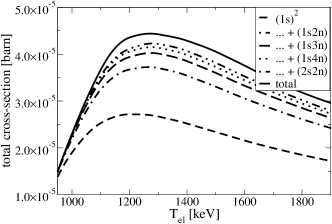
Figure 4: The total cross-section of NCDR into various bound states as a function of the kinetic energy of the incoming electron.

V Summary

In summary, the negative continuum dielectronic recombination of high–$Z$, bare ions with free electron targets has been studied within a framework of the first–order perturbation theory and Dirac’s relativistic equation. For this process, which leads to a production of a continuum–state positron and a residual helium–like ion, we have evaluated both, the angle–differential and the total cross-sections. Special attention in our theoretical analysis has been paid to the effects on these cross–sections owing to an electron transition into excited ionic states. We have demonstrated, for example, that NCDR into singly–excited $(1s\,nl_{j})$ with $n>1$ and doubly excited $(2s\,2l_{j})$ states of (finally) helium–like uranium U⁹⁰⁺ may result in a significant—up to 75 %—enhancement of the total recombination cross-section.

Despite such an enhancement, total recombination cross sections remain rather small making thus observation of the process difficult at the present–day facilities. Owing to the recent advances in ion storage ring and particle detector techniques, however, NCDR experiments are planed to be carried out at the future ion beam FAIR facility GSI (2001). One of the signatures of the NCDR process is that the projectiles change their charge state by two units. For the estimated NCDR cross sections and beam intensities of $10^{8}$ ions/second at an energy of 1.5 GeV/u (conservative estimate for the FAIR facility GSI (2001)), an event rate of about 2/10 per second can be expected for a target thickness of $10^{19}$ particle/cm² . As targets one may prefer low–$Z$ targets such as Be. Here, competitive atomic processes such as uncorrelated double electron capture might lead to a background of about one event per minute which may partially mask the original process. In order to avoid such a background an alternative experimental set–up may be considered where the emitted positron is detected in coincidence with the down–charged ions. Assuming a detector efficiency of the level of 1% about 10 coincidence events in one hour could be expected which makes NCDR process clearly observable at the future FAIR facility in Darmstadt. More detailed analysis of the various experimental scenarios as well as of the possible competitive processes is now underway and will be presented elsewhere Voitkiv et al. (2009).

VI Acknowledgments

Elucidating discussions with C. Kozhuharov are gratefully acknowledged. A.A. and A.S. acknowledge support from the Helmholtz Gemeinschaft (Nachwuchsgruppe VH–NG–421). The work of V.M.S. was supported by RFBR (Grant No. 08-02-91967) and by DFG (Grant No. 436RUS113/950/0-1).

References

- Eichler and Meyerhof (1995) J. Eichler and W. Meyerhof, Relativistic Atomic Collisions (Academic Press, San Diego, 1995).
- Eichler (2005) J. Eichler, Phys. Lett. A 347, 67 (2005).
- Baur et al. (2007) G. Baur, K. Hencken, and D. Trautmann, Physics Reports 453, 1 (2007).
- Baltz et al. (1996) A. J. Baltz, M. J. Rhoades-Brown, and J. Weneser, Phys. Rev. E 54, 4233 (1996).
- Bruce et al. (2007) R. Bruce, J. M. Jowett, S. Gilardoni, A. Drees, W. Fischer, S. Tepikian, and S. R. Klein, Physical Review Letters 99, 144801 (2007).
- Belkacem et al. (1993) A. Belkacem, H. Gould, B. Feinberg, R. Bossingham, and W. E. Meyerhof, Phys. Rev. Lett. 71, 1514 (1993).
- Vane et al. (1997) C. R. Vane, S. Datz, E. F. Deveney, P. F. Dittner, H. F. Krause, R. Schuch, H. Gao, and R. Hutton, Phys. Rev. A 56, 3682 (1997).
- Belkacem et al. (1998) A. Belkacem, N. Claytor, T. Dinneen, B. Feinberg, and H. Gould, Phys. Rev. A 58, 1253 (1998).
- Reinhardt et al. (1978) J. Reinhardt, V. Oberacker, B. Müller, W. Greiner, and G. Soff, Phys. Lett. B 178, 183 (1978).
- Müller-Nehler and Soff (1994) U. Müller-Nehler and G. Soff, Physics Reports 246, 101 (1994).
- Ionescu and Belkacem (1999) D. C. Ionescu and A. Belkacem, Physica Scripta T80, 128 (1999).
- Busic et al. (2004) O. Busic, N. Grün, and W. Scheid, Phys. Rev. A 70, 062707 (2004).
- Artemyev et al. (2003) A. N. Artemyev, T. Beier, J. Eichler, A. E. Klasnikov, C. Kozhuharov, V. M. Shabaev, T. Stöhlker, and V. A. Yerokhin, PRA 67, 052711 (2003).
- GSI (2001) Conceptual Design Report: An international accelerator facility for beams of ions and antiprotons (GSI, http://www.gsi.de/GSI-Future/cdr/, 2001).
- Artemyev et al. (2005) A. N. Artemyev, A. E. Klasnikov, T. Beier, J. Eichler, C. Kozhuharov, V. M. Shabaev, T. Stöhlker, and V. A. Yerokhin, NIMB 235, 270 (2005).
- Bjorken and Drell (1965) J. D. Bjorken and S. D. Drell, Relativistic Quantum Fields (McGraw-Hill, New York, 1965).
- Itzykson and Bernard Zuber (1980) C. Itzykson and J. Bernard Zuber, Quantum Field Theory (McGraw-Hill, New York, 1980).
- Rose (1961) M. E. Rose, Relativistic Electron Theory (John Wiley & Sons, New York, 1961).
- Salvat et al. (1995) F. Salvat, J. M. Fernández-Varea, and W. Williamson Jr., Comput. Phys. Commun. 90, 151 (1995).
- Balashov et al. (2000) V. V. Balashov, A. N. Grum-Grzhimailo, and N. M. Kabachnik, eds., Polarization and Correlation Phenomena in Atomic Collisions (Kluwer Academic Plenum Publishers, New York, 2000).
- Johnson et al. (1988) W. R. Johnson, S. A. Blundell, and J. Sapirstein, Phys. Rev. A 37, 2764 (1988).
- Dedrick (1962) K. G. Dedrick, Rev. Mod. Phys. 34, 429 (1962).
- Voitkiv et al. (2009) A. B. Voitkiv, B. Najjari, A. N. Artemyev, and A. S. Surzhykov, in preparation.