Statistics of the two-point transmission at Anderson localization transitions
Abstract
At Anderson critical points, the statistics of the two-point transmission for disordered samples of linear size is expected to be multifractal with the following properties [Janssen et al PRB 59, 15836 (1999)] : (i) the probability to have behaves as , where the multifractal spectrum terminates at as a consequence of the physical bound ; (ii) the exponents that govern the moments become frozen above some threshold: , i.e. all moments of order are governed by the measure of the rare samples having a finite transmission (). In the present paper, we test numerically these predictions for the ensemble of power-law random banded matrices, where the random hopping decays as a power-law . This model is known to present an Anderson transition at between localized () and extended () states, with critical properties that depend continuously on the parameter . Our numerical results for the multifractal spectra for various are in agreement with the relation in terms of the singularity spectrum of individual critical eigenfunctions, in particular the typical exponents are related via the relation . We also discuss the statistics of the two-point transmission in the delocalized phase and in the localized phase.
I Introduction
Since its discovery fifty years ago [1], Anderson localization has remained a very active field of research (see the reviews [2, 3, 4, 5, 6, 7, 8]). One of the most important property of Anderson localization transitions is that critical eigenfunctions are described by a multifractal spectrum defined as follows (for more details see for instance the reviews [6, 8]): in a sample of size , the number of points where the weight scales as behaves as
| (1) |
The inverse participation ratios (I.P.R.s) can be then rewritten as an integral over
| (2) |
The exponent can be obtained via a saddle-point calculation in , and one obtains the Legendre transform formula [6, 8]
| (3) |
These scaling behaviors, which concern individual eigenstates , can be translated for the local density of states
| (4) |
as follows : for large , when the energy levels become dense, the sum of Eq. 4 scales as
| (5) |
and its moments involve the exponents introduced in Eq. 2
| (6) |
These notions concern one-point functions, and it is natural to consider also the statistics of two-point functions. In particular, a very interesting observable to characterize Anderson transitions is the two-point transmission when the disordered sample of size is attached to one incoming wire and one outcoming wire [9, 28] : (i) it remains finite in the thermodynamic limit only in the delocalized phase, so that it represents an appropriate order parameter for the conducting/non-conducting transition; (ii) exactly at criticality, it displays multifractal properties in direct correspondence with the multifractality of critical eigenstates, i.e. it displays strong fluctuations that are not captured by more global definitions of conductance. More precisely, as first discussed in [9] for the special case of the two dimensional quantum Hall transition, the critical probability distribution of the two-point transmission takes the form
| (7) |
and its moments involve non-trivial exponents
| (8) |
As stressed in [9], the physical bound on the transmission implies that the multifractal spectrum exists only for , and this termination at leads to a complete freezing of the moments exponents
| (9) |
at the value where the saddle-point of the integral of Eq. 8 vanishes . It is very natural to expect some relation between the two multifractal spectra and , and the possibility proposed in [9] is that before the freezing of Eq. 9 occurs, the transmission should scale as the product of two independent local densities of states (Eq. 6)
| (10) |
We refer to [9] for physical arguments in favor of this relation. Equations 9 and 10 for the moments exponents are equivalent to following relation between the two multifractal spectra
| (11) |
In this paper, our aim is to test numerically these predictions for the statistics of the two-point transmission at the critical points of the Power-law Random Banded Matrix (PRBM) model, where one parameter allows to interpolate continuously between weak multifractality and strong multifractality. We will also discuss the statistics of the two-point transmission off criticality.
The paper is organized as follows. In section II, we introduce the PRBM model and the scattering geometry used to define the two-point transmission. In Section III, we present our numerical results concerning the multifractal statistics of the two-point transmission at criticality. We then discuss the statistics of the two-point transmission in the localized phase (Section IV) and in the delocalized phase (Section V) respectively. Our conclusions are summarized in section VI. The appendices A and B contain more details on the numerical computations.
II Model and observables
Beside the usual short-range Anderson tight-binding model in finite dimension , other models displaying Anderson localization have been studied, in particular the Power-law Random Banded Matrix (PRBM) model, which can be viewed as a one-dimensional model with long-ranged random hopping decaying as a power-law of the distance with exponent and parameter (see below for a more precise definition of the model). The Anderson transition at between localized () and extended () states has been characterized in [10] via a mapping onto a non-linear sigma-model. The properties of the critical points at have been then much studied, in particular the statistics of eigenvalues [11, 12, 13], and the multifractality of eigenfunctions [14, 15, 16, 17, 18, 19], including boundary multifractality [20]. The statistics of scattering phases, Wigner delay times and resonance widths in the presence of one external wire have been discussed in [21, 22]. Related studies concern dynamical aspects [23], the case with no on-site energies [24], and the case of power-law hopping terms in dimension [25, 26, 27]. In this paper, we consider the PRBM in a ring geometry (dimension with periodic boundary conditions) in the presence of two external wires to measure the transmission properties.
II.1 Power-law random banded matrices with periodic boundary conditions
We consider sites in a ring geometry with periodic boundary conditions, where the appropriate distance between the sites and is defined as [14]
| (12) |
The ensemble of power-law random banded matrices of size is then defined as follows : the matrix elements are independent Gaussian variables of zero-mean and of variance
| (13) |
The most important properties of this model are the following. The value of the exponent determines the localization properties [10] : for states are localized with integrable power-law tails, whereas for states are delocalized. At criticality , states become multifractal [14, 15, 16, 17] and exponents depend continuously of the parameter , which plays a role analog to the dimension in short-range Anderson transitions [14] : the limit corresponds to weak multifractality ( analogous to the case ) and can be studied via the mapping onto a non-linear sigma-model [10], whereas the case corresponds to strong multifractality ( analogous to the case of high dimension ) and can be studied via Levitov renormalization [34, 14]. Other values of have been studied numerically [14, 15, 16, 17].
II.2 Scattering geometry used to define to two-point transmission
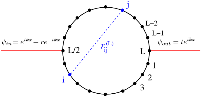
In quantum coherent problems, the most appropriate characterization of transport properties consists in defining a scattering problem where the disordered sample is linked to incoming wires and outgoing wires, and in studying the reflection and transmission coefficients. This scattering theory definition of transport, first introduced by Landauer [29], has been often used for one-dimensional systems [30, 31, 32] and has been generalized to higher dimensionalities and multi-probe measurements (see the review [33]). In the present paper, we focus on the Landauer transmission for the scattering problem shown on Fig. 1: an incoming wire is attached at the site and an outgoing wire is attached at the site . We are thus interested into the eigenstate that satisfies the Schrödinger equation
| (14) |
inside the disorder sample characterized by the random , and in the perfect wires characterized by no on-site energy and by hopping unity between nearest neighbors. Within these perfect wires, one requires the plane-wave forms
| (15) |
These boundary conditions define the reflection amplitude of the incoming wire and the transmission amplitude of the outgoing wire. The Landauer transmission
| (16) |
is then a number in the interval . More details on the numerical computation of the transmission in a given sample are given in Appendix A.
To satisfy the Schrödinger Equation of Eq. 14 within the wires with the forms of Eq. 15, one has the following relation between the energy and the wave vector
| (17) |
To simplify the discussion, we will focus in this paper on the case of zero-energy (wave-vector ) that corresponds to the center of the band.
In the following, we study numerically the statistical properties of the Landauer transmission for rings of size with corresponding statistics of independent samples. For typical values, the number of samples is sufficient even for the bigger sizes, whereas for the measure of multifractal spectrum, we have used only the smaller sizes where the statistics of samples was sufficient to measure correctly the rare events.
III Statistics of the two-point transmission at criticality ()
As recalled in the Introduction, the two-point transmission is expected to display multifractal statistics at criticality [9]. We first focus on the scaling of the typical transmission before we turn to the multifractal spectrum and the moments of arbitrary order.
III.1 Typical transmission at criticality ()
As discussed in [9, 28], the typical transmission
| (18) |
is expected to decay at criticality with some power-law
| (19) |
where the exponent is directly related via the relation
| (20) |
to the typical exponent that characterizes the typical weight of eigenfunctions
| (21) |
This typical value corresponds to the maximum value of the multifractal spectrum introduced in Eq. 1 . (Note that in [9, 28]), is denoted by and by . Here we have chosen to use the explicit notation ’typ’ for clarity).
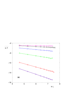
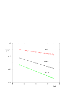
For the PRBM considered here, the dimension is , and critical exponents depend continuously on . We show on Fig. 2 (a) the as a function of : the slopes allows to measure the exponents
| (22) |
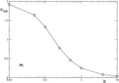
On Fig. 2 (b), we show how the exponent depends on . The values we have measured are listed in Table 1, together with the corresponding values of obtained via Eq. 20 : these values of are compatible with the values of the maxima of the multifractal spectrum of critical eigenstates measured in [14] (see Fig. 2 and Fig. 6 of [14]) and in [19] (see Fig. 2 and Fig. 3 of [19]).
b 0.01 0.05 0.1 0.25 0.5 1 4 10 2 1.92 1.64 1.33 0.77 0.46 0.25 0.08 0.04 0 2 1.96 1.82 1.66 1.38 1.23 1.12 1.04 1.02 1
The two limits and can be understood as follows. The case corresponds to very weak multifractality with the typical exponent [14, 19]. Equation 20 yields that the critical exponent of the typical transmission becomes arbitrary small in the limit
| (23) |
The opposite limit corresponds to very strong multifractality with the typical exponent [14, 19]. Equation 20 thus yields
| (24) |
III.2 Multifractal spectrum with termination at
As recalled in the introduction, the statistics of the two-point transmission is expected to be multifractal at criticality, as a consequence of the multifractal character of critical eigenfunctions [9]. For the PRBM, the multifractal spectrum of Eq. 7 will depend continuously on the parameter
| (25) |
Since it describes a probability, the multifractal spectrum satisfies , and the maximal value is reached only for the typical value discussed above
| (26) |
The relation of Eq. 20 between the two typical exponents and is expected to come from the more general relation of Eq. 11 between the two multifractal spectra and
| (27) |
An essential property of the spectrum is that it exists only for as a consequence of the physical bound , so that it terminates at at the finite value
| (28) |
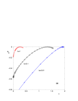
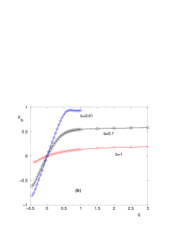
To measure numerically the multifractal spectrum , we have used the standard method based on -measures of Ref. [35] (see more details in Appendix B). To show how the parameter allows to interpolate between weak multifractality and strong multifractality, we compare on Fig. 3 (a) the multifractal spectra for the three values , and . For instance for the value , the termination value we measure is in agreement via Eq. 28 with the value of Fig. 6 of [14] and Fig. 2 of [19].
III.3 Freezing transition of the moments exponents
As usual, the multifractal statistics of Eq. 25 has for consequence that the moments of arbitrary order
| (29) |
are governed by non-trivial exponents that can be obtained via the saddle-point calculation
| (30) |
As long as the saddle-point value satisfies , can be obtained via the usual Legendre transform formula
| (31) |
However above some threshold , the saddle-point value will saturate to the boundary value
| (32) |
and the exponent will saturate to the value
| (33) |
This freezing phenomenon of at predicted in [9] means that all moments of order are dominated by the rare events corresponding to a finite transmission , whose measure behaves as .
We show on Fig. 3 (a) the moments exponents for the three values , and . For instance for , the freezing value corresponds to the termination value of Fig. 3 (a).
It turns out that for Anderson transitions, a special symmetry of the multifractal spectrum has been proposed (see [19, 36] and references therein) that relates the regions and via the relation . This symmetry then fixes the value of where or equivalently to be exactly
| (34) |
Numerically, it is difficult to measure precisely the value where the exponents become completely frozen as a consequence of finite-size corrections around this phase transition point for the , as already found for the quantum Hall transition in [9]. However Fig. 3 (b) shows that in the limit of strong multifractality (), the numerical saturation value is not far from the theoretical prediction of Eq. 34.
IV Statistics of the two-point transmission in the localized phase ()
IV.1 Typical transmission in the localized phase
In usual short-range models, the localized phase is characterized by exponentially localized wavefunctions, whereas in the presence of power-law hoppings, localized wavefunction can only decay with power-law integrable tails. For the PRBM, it is moreover expected that the asymptotic decay is actually given exactly by the power-law of Eq. 13 for the hopping term defining the model [10] : . As a consequence in the localized phase , one expects the typical decay
| (35) |
As shown on Fig. 4, we have checked this power-law decay of the typical transmission for the case and the two values , .
IV.2 Histogram of in the localized phase ()
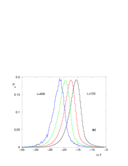
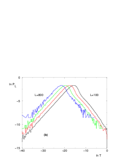
We show on Fig. 5 the histograms of for the four sizes in the localized phase for the case : these data seem to indicate that as grows, the probability distribution shifts to the left while keeping a fixed shape. This means that the relative variable with respect to the typical value discussed above (see Eq. 35) remains a finite variable as . In addition, the left tail is governed by the exponent
| (36) |
or equivalently after the change of variable
| (37) |
These properties can be understood by the following simple argument. In the localized phase , one may assume that for large , the transmission is dominated by the direct hopping term (see Fig. 1)
| (38) |
where is a Gaussian variable of zero mean and variance unity (see Eq. 13). In particular, its probability density is finite near the origin . The change of variable
| (39) |
then yields the power-law of Eq. 37.
V Statistics of the two-point transmission in the delocalized phase ()
V.1 Typical transmission in the delocalized phase
In the delocalized phase, the eigenfunctions are not multifractal anymore, but monofractal with the single value for the weight As a consequence, the typical transmission is expected to remain finite as [9] (in Eq. 20, the case yields )
| (40) |
The two-point transmission is thus a good order parameter of the transport properties [9].
V.2 Histogram of in the delocalized phase
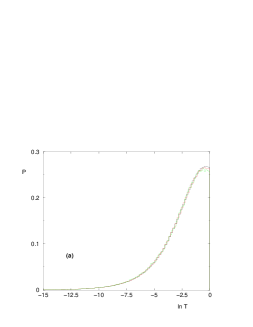
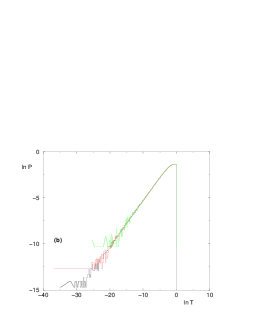
We find that the whole probability distribution converges for large towards a fixed distribution . As an example, we show on Fig. 6 the histograms of for three sizes concerning the case and . These histograms stops at as a consequence of the bound . In the region of very small transmission the log-log plot of Fig. 6 (b) indicates the same form as in Eq. 36
| (41) |
or equivalently after a change of variable
| (42) |
As explained around Eq. 39, this power-law behavior simply means that the transmission can be written as the square of some random variable that has a finite probability density at the origin . This means that all negative moments of order actually diverge in the delocalized phase
| (43) |
VI Conclusions and perspectives
In this paper, we have studied numerically the statistics of the two-point transmission as a function of the size in the PRBM model that depends on two parameters :
(i) in the delocalized phase (), we have found that the probability distribution of converges for towards a law presenting the power-law of Eq. 42 for .
(ii) in the localized phase (), we have found that the probability distribution keeps a fixed shape around the typical value as grows, and the typical value decays only as the power-law of Eq. 35 as a consequence of the presence of power-law hoppings.
(iii) exactly at criticality (), the statistics of the two-point transmission is multifractal : we have measured the multifractal spectra as well as the moments exponents for various values of the parameter that allows to interpolate between weak multifractality and strong multifractality. We have tested in detail the various expectations of Ref. [9] concerning the termination of at , the freezing of above some value , and the relations with the singularity spectrum of individual critical eigenstates.
To finish, we should stress that the relation of Eq. 11 relates the transmission between two ’bulk points’ to the ’bulk multifractal spectrum’ . In localization models, it is however more usual to attach leads to the boundaries of the disordered sample : then the statistics of the two-point transmission is related to the ’surface multifractal spectrum’ as will be discussed in more details elsewhere [37]. We will also discuss in [37] the statistical properties of the transmission for various scattering geometries involving a large number of wires.
Appendix A Computation of the two-point transmission in each sample
To compute the transmission of a given sample via Eq. 16, we have to solve the Schödinger problem of Eq. 14 with the scattering boundary conditions of Eq. 15. This can be decomposed in two steps as follows.
A.1 Recursive elimination of the ’interior sites’
The first step consists in the iterative elimination of the ’interior sites’, i.e. of all the sites not connected to the external wires (see Fig. 1). To eliminate the site , one uses the Schödinger Eq. 14 projected on this site
| (44) |
to make the substitution
| (45) |
in all other remaining equations. Then from the point of view of remaining sites, the hoppings are renormalized according to
| (46) |
This procedure is stopped when the only remaining sites are the two sites and connected to the external wires (see Fig. 1) : the three real remaining parameters are the renormalized hopping and the two renormalized on-site energies ,
A.2 Effective scattering problems for the two boundary sites
The second step consists in solving the scattering problem for the two boundary sites and connected to the external wires (see Fig. 1) with the renormalized parameters obtained above. The Schödinger Eq. 14 projected on the boundary sites and read
| (47) |
The boundary conditions of Eq. 15 fixes the following ratio on the outgoing wire
| (48) |
The following ratio
| (49) |
concerning the incoming wire can be then computed in terms of the three real renormalized parameters
| (50) |
The reflexion coefficient of Eq. 15 is then obtained as
| (51) |
yielding the transmission of Eq. 16.
Appendix B Computation of the multifractal spectrum over the samples
To measure numerically the multifractal spectrum of Eq. 7 that characterizes the statistics of the transmission over the samples of size , we have used the standard method based on -measures of Ref. [35]. More precisely, for various sizes , we have measured the transmission for a number of independent samples . Then for various values of , we have computed the moments of Eq. 8
| (52) |
to extract the moments exponents as the slope of the log-log plot
| (53) |
We have also computed the auxiliary observables
| (54) |
and
| (55) |
to obtain and as the slopes of
| (56) |
and
| (57) |
This yields a parametric plot in of the multifractal spectrum : on Figure 3 (a), each circle of coordinate corresponds to a value of .
References
- [1] P.W. Anderson, Phys. Rev. 109, 1492 (1958).
- [2] D.J. Thouless, Phys. Rep. 13, 93 (1974) ; D.J. Thouless, in “Ill Condensed Matter” (Les Houches 1978), Eds R. Balian et al. North-Holland, Amsterdam (1979).
- [3] B. Souillard, in “ Chance and Matter” (Les Houches 1986), Eds J. Souletie et al. North-Holland, Amsterdam (1987).
- [4] I.M. Lifshitz, S.A. Gredeskul and L.A. Pastur, “Introduction to the theory of disordered systems” (Wiley, NY, 1988).
- [5] B. Kramer and A. MacKinnon, Rep. Prog. Phys. 56, 1469 (1993).
- [6] M. Janssen, Phys. Rep. 295, 1 (1998).
- [7] P. Markos, Acta Physica Slovaca 56, 561 (2006).
- [8] F. Evers and A.D. Mirlin, Rev. Mod. Phys. 80, 1355 (2008).
- [9] M. Janssen, M. Metzler and M.R. Zirnbauer, Phys. Rev. B 59, 15836 (1999).
- [10] A.D. Mirlin et al, Phys. Rev. E 54, 3221 (1996).
- [11] I. Varga and D. Braun, Phys. Rev. B 61, R11859 (2000).
- [12] V.E. Kravtsov et al, J. Phys. A 39, 2021 (2006).
- [13] A.M. Garcia-Garcia, Phys. Rev. E 73, 026213 (2006).
- [14] F. Evers and A. D. Mirlin Phys. Rev. Lett. 84, 3690 (2000); A.D. Mirlin and F. Evers, Phys. Rev. B 62, 7920 (2000).
- [15] E. Cuevas, V. Gasparian and M. Ortuno, Phys. Rev. Lett. 87, 056601 (2001).
- [16] E. Cuevas et al, Phys. Rev. Lett. 88, 016401 (2001).
- [17] I. Varga, Phys. Rev. B 66, 094201 (2002).
- [18] E. Cuevas, Phys. Rev. B 68, 024206 (2003).
- [19] A. D. Mirlin et al, Phys. Rev. Lett 97, 046803 (2006).
- [20] A. Mildenberger et al, Phys. Rev. B 75, 094204 (2007).
- [21] J.A. Mendez-Bermudez and T. Kottos, Phys. Rev. B 72, 064108 (2005).
- [22] J.A. Mendez-Bermudez and I. Varga, Phys. Rev. B 74, 125114 (2006).
- [23] R.P.A. Lima et al, Phys. Rev. B 71, 235112 (2005).
- [24] R.P.A. Lima et al, Phys. Rev. B 69, 165117 (2004).
- [25] H. Potempa and L. Schweitzer, Phys. Rev. B 65, 201105(R) (2002).
- [26] E. Cuevas, Phys. Stat. Sol. 241, 2109 (2004).
- [27] E. Cuevas, Phys. Rev. B 71, 024205 (2005).
- [28] F. Evers, A. Mildenberger and A. D. Mirlin, Phys. Stat. Sol. 245, 284 (2008).
- [29] R. Landauer, Philos. Mag. 21, 863 (1970).
- [30] P. W. Anderson, D. J. Thouless, E. Abrahams and D. S. Fisher Phys. Rev. B 22, 3519 (1980).
- [31] P. W. Anderson and P.A. Lee, Suppl. Prog. Theor. Phys. 69, 212 (1980).
- [32] J.M. Luck, “Systèmes désordonnés unidimensionnels” , Alea Saclay (1992).
- [33] A.D. Stone and A. Szafer, IBM J. Res. Dev. 32, 384 (1988).
- [34] L.S. Levitov, Europhys. Lett. 9, 83 (1989); L.S. Levitov, Phys. Rev. Lett. 64, 547 (1990); B.L. Altshuler and L.S. Levitov, Phys. Rep. 288, 487 (1997); L.S. Levitov, Ann. Phys. (Leipzig) 8, 5, 507 (1999)
- [35] A. Chhabra and R.V. Jensen, Phys. Rev. Lett. 62, 1327 (1989).
- [36] L.J. Vasquez, A. Rodriguez and R.A. Romer, Phys. Rev. B 78, 195106 (2008); A. Rodriguez, L.J. Vasquez and R.A. Romer, Phys. Rev. B 78, 195107 (2008); A. Rodriguez, L.J. Vasquez and R.A. Romer, arxiv:0812.1654.
- [37] C. Monthus and T. Garel, in preparation.