Conformal tightness of holographic scaling in black hole thermodynamics

Abstract

The near-horizon conformal symmetry of nonextremal black holes is shown to be a mandatory ingredient for the holographic scaling of the scalar-field contribution to the black hole entropy. This conformal tightness is revealed by semiclassical first-principle scaling arguments through an analysis of the multiplicative factors in the entropy due to the radial and angular degrees of freedom associated with a scalar field. Specifically, the conformal SO(2,1) invariance of the radial degree of freedom conspires with the area proportionality of the angular momentum sums to yield a robust holographic outcome.

1 Introduction

The holographic scaling of the Bekenstein-Hawking black hole entropy [1]:

$$S_{\rm BH}\propto{\mathcal{A}}\;,$$ (1.1)

i.e., its proportionality with the area ${\mathcal{A}}$ of the event horizon, is one of the central results of contemporary theoretical physics and a litmus test for quantum theories of gravity [2]. In essence, the apparent universality of the area law suggests that the horizon encodes information at the quantum level [3, 2, 4] (in the form of a holographic principle [5]).

In the search for patterns that may elucidate this intriguing property, several lines of research have focused on the existence of a near-horizon conformal symmetry [6, 7, 8] as a ubiquitous property of black hole thermodynamics. Most remarkably, in Refs. [9, 10], the thermodynamics is explicitly connected with the underlying near-horizon conformal field theory through the Cardy formula. Alternatively, within a general framework inspired by the brick-wall model [3], conformal quantum mechanics (CQM) has been directly linked with the thermodynamic properties [11, 12] by considering a scalar field ($D\geq 4$)

$$S=-\frac{1}{2}\int d^{D}x\,\sqrt{-g}\,\left[g^{\mu\nu}\,\nabla_{\mu}\Phi\,\nabla_{\nu}\Phi+m^{2}\Phi^{2}+\xi R\Phi^{2}\right]\;,$$ (1.2)

in a given gravitational background. Admittedly, in the form derived from the action (1.2), it only yields the scalar field contribution to the entropy of the black hole, though extensions to higher-spin fields are in progress. In addition and most importantly, a complete understanding of the predominant role of CQM in the determination of the thermodynamic properties of black holes has not yet been fully achieved, especially vis-à-vis the physical and geometric meaning of the underlying conformal symmetry. It should be noticed that semiclassical methods, based on quantum fields in the black hole background, include both the brick wall approach or thermal atmosphere proposal, and the entanglement entropy approach [14, 15]. Moreover, the brick wall and entanglement entropies are essentially equivalent .

Our paper provides further strong evidence of the conformal characterization of black hole thermodynamics by focusing, for scalar fields, on a critical question regarding the entropy, while the more complex issue of the role played by conformal symmetry in the Hawking effect is left for a forthcoming publication. In effect, the apparent central role of CQM is highlighted by the conformal determination of the Hawking temperature; however, the angular-momentum sums in semiclassical treatments of quantum field theory also seem to be an essential ingredient in the derivation of the Bekenstein-Hawking entropy $S_{\rm BH}$. Thus, the question we now formulate is whether or not the area law, equation (1.1), for the entropy is a direct consequence of the statistical counting of the angular degrees of freedom, independently of the attendant near-horizon conformal symmetry. In other words, is the scaling of the entropy critically constrained by the conformal nature of the radial degree of freedom, above and beyond the role played by the angular degrees of freedom? Or, by contrast, does the conformal symmetry merely provide circumstantial evidence rather than logical necessity for the holographic nature of the entropy? Again, for the sake of simplicity, we will only focus on the scalar-field contribution to the entropy. This issue is further motivated by early back-of-the-envelope phase-space arguments (see [17, 18] and [19]), which appear to suggest the accidental nature of the conformal symmetry, with $S_{\rm BH}$ in equation (1.1) arising from the straightforward angular summation of degrees of freedom. However, such arguments rely on implicit assumptions regarding the radial degrees of freedom—incidentally, related observations were made in Ref. [20], where additional issues concerning the nature of the horizon were also addressed. Specifically, as we explicitly show below, the radial part of the metric yields a multiplicative complementary piece in the phase-space counting for the scalar field, with ‘radial conformality’ of the near-horizon physics guaranteeing the preservation of holographic scaling. What comes out from this analysis is further evidence of the governing role played by CQM—at least for scalar fields: first, in the direct determination of the Hawking temperature; and second, as the central result of our paper, in the statistical counting of the relevant near-horizon degrees of freedom. Most importantly, the robustness of these results can be tested by considering a larger class of metrics and displaying what may be dubbed conformal tightness:

Near-horizon conformal behavior—as described by conformal quantum mechanics—is a necessary condition for the thermal properties of black holes. Any non-conformal modification of the metric spoils the thermal identification of the Hawking temperature and breaks the holographic scaling or Bekenstein-Hawking area law for the entropy.

Our proofs rely on properties of the metric, via an argument that traces the apparent origin of the holographic scaling of the entropy to the angular degrees of freedom. A first step is taken in section 2, then followed by a more precise characterization of conformal tightness in section 3, and further context in section 4. Additional topics in the appendices include the computation of the near-horizon spectral integrals (A) and alternative phase-space arguments (B).

2 Origin of the area law: basic setup for generalized Schwarzschild metrics

Our stated goal is to highlight the ‘conformal emergence’ of the area scaling of the black hole entropy, by considering a quantum scalar field probe with action (1.2) in a gravitational background of the form

$$ds^{2}=-f(r)\,dt^{2}+\left[f(r)\right]^{-1}\,dr^{2}+r^{2}\,d\Omega^{2}_{(D-2)}\;$$ (2.1)

[in which $d\Omega^{2}_{(D-2)}$ is the metric on the unit $(D-2)$-spheres, $S^{D-2}$, that foliate the spacetime manifold and the metric conventions of Ref. [21] are used]. Equation (2.1) represents a static-coordinate description or generalized Schwarzschild chart for a generic static geometry. The corresponding family of spacetimes includes the Reissner-Nordström geometries in $D$ spacetime dimensions [22], and possibly extensions with a cosmological constant. In Section 3, we generalize this family to emphasize that the conformal nature of the thermodynamics appears to be a fairly universal property of black holes. In principle, the basic results of conformal tightness could be further generalized to axisymmetric stationary spacetimes, as will be discussed in a forthcoming paper. As is well known, for static spacetimes, there exists a coordinate frame in which the timelike coordinate $t$ is associated with the Killing vector field $\mbox{\boldmath$\xi$ }\!=\partial_{t}$ that is hypersurface orthogonal [23], and for which the metric can be adapted to $ds^{2}=g_{00}\,dt^{2}+\gamma_{ij}dx^{i}dx^{j}$, where $g_{00}$ and the spatial metric $\gamma_{ij}$ are time independent; this includes equation (2.1) and the generalization of section 3. The Killing vector $\xi$ permits the introduction of a Killing horizon ${\mathcal{H}}$ where the surface gravity $\kappa$ is defined in purely geometric terms [23],

$$\kappa\stackrel{{\scriptstyle(\mathcal{H})}}{{=}}\frac{1}{2}\sqrt{-\frac{1}{2}\nabla_{\alpha}\xi_{\beta}\nabla^{\alpha}\xi^{\beta}}\;.$$ (2.2)

In addition, for the particular class of metrics (2.1),

$$\kappa\stackrel{{\scriptstyle(\cal H)}}{{=}}\sqrt{\nabla_{\alpha}V(x)\nabla^{\alpha}V(x)}\stackrel{{\scriptstyle(\mathcal{H})}}{{=}}\frac{1}{2}\,f^{\prime}_{+}\,,$$ (2.3)

in which $V(x)\equiv\sqrt{-\xi^{\mu}\xi_{\mu}}=\sqrt{f(r)}$ and all the derivatives are evaluated at $\mathcal{H}$, in terms of $f_{+}^{\prime}=f^{\prime}(r_{+})$, using the standard notation $r=r_{+}$ for the outer event horizon, identified as the largest root of the equation $f(r)=0$. In the nonextremal case: $f^{\prime}_{+}\neq 0$, which is the focus of this work, the surface gravity has a well-defined nonzero value (while the extremal case will be tackled elsewhere, in view of its subtle analytical properties [4]).

It should be noticed that the Hawking temperature can be computed for the metrics (2.1) from the removal of the conical singularity, with the result

$$\beta=\frac{2\pi}{\kappa}$$ (2.4)

for the inverse temperature; see section 3 for a more detailed account for a generalized class of metrics. As a general methodology, the relations (2.3) and (2.4)—properly generalized in section 3—will be systematically used to simplify the interpretation of the statements and calculations; consequently, our focus will be on addressing the questions stated in section 1, especially on the conformal nature of the entropy.

To shed light on the origin of the holographic expression (1.1) we will often invoke scaling relationships arising from the relevant physics, e.g., $\kappa\simeq f_{+}^{\prime}$. While the complete analytical results are displayed in subsection 2.1, the scaling equations will help elucidate the role played by the different degrees of freedom in the ensuing holographic behavior.

2.1 Origin of the area law: detailed computation in generalized Schwarzschild coordinates

The basic strategy is to identify the origin of the area law for the entropy through the bookkeeping of the relevant degrees of freedom. The standard procedure is based on the Fourier expansion of the quantum field with a complete set of orthonormal modes $\Phi_{\omega_{s},s}=\phi_{s}(r,\Omega)\,e^{-i\omega_{s}t}$ that satisfy the Klein-Gordon equation in the black-hole background,

$$\frac{1}{\sqrt{-g}}\partial_{\mu}\left(\sqrt{-g}\,g^{\mu\nu}\,\partial_{\nu}\Phi\right)-\left(m^{2}+\xi R\right)\Phi=0\;,$$ (2.5)

where the terms above include the d’Alembert-Beltrami operator, the mass term, and a possible coupling to the Ricci scalar $R$, as described by the action (1.2). In this decomposition, for the static metric (2.1) in generalized Schwarzschild coordinates $(t,r,\Omega)$, the factorization $\Phi_{\omega_{s}}=\phi_{s}(r,\Omega)\,e^{-i\omega_{s}t}$ is based on the Lie-derivative equation ${\mathcal{L}}_{\mbox{\boldmath${\scriptstyle\xi}$ }}\Phi_{\omega}=-i\omega\Phi_{\omega}$ with the Killing vector $\xi$ (for positive-frequency modes, and the corresponding conjugate relation for negative-frequency modes). Thus,

$$\Phi(t,r,\Omega)=\sum_{s}\left[a_{s}\,\phi_{s}(r,\Omega)\,e^{-i\omega_{s}t}+a^{\dagger}_{s}\,\phi^{*}_{s}(r,\Omega)\,e^{i\omega_{s}t}\right]\;,$$ (2.6)

where the creation and annihilation operators $a^{\dagger}_{s}$ and $a_{s}$ satisfy the canonical commutation relations and $s=(n,l,{\bf m})$ labels the radial and angular eigenvalues—in particular, the states in the ensuing Fock space are generated according to their occupation numbers per mode from the Boulware vacuum [24]. Equation (2.5) can then be recast in the spatially-reduced form (with an operator $\hat{{\mathcal{A}}}$)

$$\hat{{\mathcal{A}}}\,\Phi=\omega^{2}\,\Phi\;,$$ (2.7)

after the Fourier frequency decomposition above is enforced (i.e., $\partial_{t}^{2}\rightarrow-\omega^{2}$). The spatial part of each mode is further rewritten in Liouville normal form [11] by the substitution $\phi(r,\Omega)=Y_{l{\bf m}}\big{(}\Omega\big{)}\,u(r)\,[f(r)]^{-1/2}\,r^{-(D-2)/2}$, where the angular dependence of the ultraspherical harmonics $Y_{l{\bf m}}\big{(}\Omega\big{)}$ (with eigenvalues $\lambda_{l,D}=l(l+D-3)$) supplements the normal radial behavior

$$u^{\prime\prime}(r)-V_{\rm eff}(r;\omega,\alpha_{l,D})\,u(r)=0\;.$$ (2.8)

In equation (2.8), the primes stand for radial derivatives and $V_{\rm eff}(r)$ is interpreted as an effective gravitational potential. Defining

$$\alpha_{l,D}=l(l+D-3)+\nu^{2}=\left(l+\frac{D-3}{2}\right)^{2}\;,$$ (2.9)

with $\nu=(D-3)/2$, which yields the angular momentum eigenvalues for each dimensionality $D$, and $\Theta=\omega/2\kappa$, then, the dominant near-horizon orders of the effective interaction are 

$$V_{\rm eff}(r;\omega,\alpha_{l,D})\stackrel{{\scriptstyle(\mathcal{H})}}{{\sim}}-\left(\Theta^{2}+\frac{1}{4}\right)\frac{1}{x^{2}}+\frac{\alpha_{l,D}}{2\kappa\,r_{+}^{2}}\frac{1}{x}\;$$ (2.10)

[up to terms $O(x)$], where $x=r-r_{+}$ and hereafter we use the symbol $\stackrel{{\scriptstyle(\mathcal{H})}}{{\sim}}$ for the near-horizon expansion with respect to the variable $x$, which displays the typical pattern shown in Figure 1 .

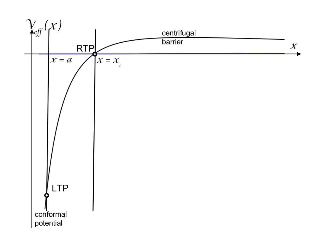
Figure 1: Near-horizon effective gravitational potential $V_{\rm eff}$ from equation (2.10), showing the interplay between the angular-momentum and conformal terms. The WKB left and right turning points: $x=a$ and $x=x_{1}$, represented by small circles, are labeled LTP and RTP.

In particular, the SO(2,1) conformal symmetry [25] under scrutiny is displayed by the leading term in equation (2.10), which amounts to the scale invariant potential $V_{\rm eff}\stackrel{{\scriptstyle(\mathcal{H})}}{{\sim}}\left.V_{\rm eff}\right|_{\rm CQM}=-\left(\Theta^{2}+1/4\right)/x^{2}$, i.e., it has same degree of homogeneity as the derivative term in equation (2.8). The ‘conformal parameter’ $\Theta$ characterizes the effective coupling strength of CQM [26, 27] and determines the Hawking temperature [28] in a unique manner [29]. However, the explicit form of the effective gravitational potential in equation (2.10) also reveals that the naive power counting with respect to $1/x$ breaks down due to the competing interplay between the two leading terms in the near-horizon expansion:

(i) The purely conformal potential $\left.V_{\rm eff}\right|_{\rm CQM}\propto-1/x^{2}$, which carries the radial degrees of freedom, is strictly dominant for low angular momenta $\alpha\equiv\alpha_{l,D}$.

(ii) The centrifugal potential term $\alpha/\left(fr^{2}\right)\propto 1/x$, which carries the angular degrees of freedom, becomes comparable to the conformal interaction for high angular momenta $\alpha$.

Evidently, this interplay is the key to answering the questions posed in section 1, regarding the relative roles played by the angular and radial degrees of freedom.

With the above considerations in mind, we seek to reformulate the thermodynamics within this framework, in purely conformal terms. In this program, the critical components of the entropy calculation involve the sequential computation of the following quantities: the spectral function, the entropy, and Planck-scale renormalization.

First, the computation of the spectral function $N(\omega)$ from the near-horizon effective gravitational potential (2.10) can be accomplished either by WKB or phase-space methods [11, 12], and also via the heat-kernel approach [30]. For our presentation in this section, the competition between the angular-momentum degrees of freedom and the leading near-horizon (conformal) effective potential is most clearly seen in its one-dimensional WKB form, which furnishes the asymptotically exact ‘spectral integral’

$$\!\!\!\!\!\!\!\!\!\!\!\!N(\omega)\stackrel{{\scriptstyle(\mathcal{H})}}{{\sim}}\frac{\Theta}{\pi\,\Gamma(D-2)}\int_{0}^{\alpha_{\rm max}(a)}d\alpha\,\alpha^{D/2-2}\,\int_{a}^{x_{1}(\alpha)}\frac{dx}{x}\,\sqrt{1-\frac{\alpha}{2\kappa r_{+}^{2}\,\Theta^{2}}\,x}\;$$ (2.11)

as the near-horizon limit of the WKB algorithm (1.1) further discussed in A. In equation (2.11), $a$ is a coordinate cutoff defining the left turning point of the potential (2.10) with ‘zero effective energy,’ while $x_{1}=r_{1}-r_{+}$ is the root of the radicand associated with its right turning point: $x_{1}(\alpha)=2\kappa r_{+}^{2}\,\Theta^{2}/\alpha$ and the angular momentum upper bound $\alpha_{\rm max}(a)=2\kappa r_{+}^{2}\,\Theta^{2}/a$ corresponds to the left-right turning-point orientation $a\leq x_{1}(\alpha)$. An alternative phase-derivation is presented in B. The ‘conformal measure’ $dx/x$ of the radial integration in equation (2.11) plays a key role in our derivation and is related to the scale-invariant radial measure used in Ref. [20].

Second, the computation of the entropy itself can be performed for the field (1.2) with the canonical-ensemble spectral rule [11, 12]

$$S=-\int_{0}^{\infty}d\omega\,\ln(1-e^{-\beta\omega})\,\left[\left(\omega\frac{d}{d\omega}+2\right)\frac{dN(\omega)}{d\omega}\right]\;,$$ (2.12)

which amounts to a thermal free-field distribution of independent modes at inverse temperature $\beta$, with canonical partition function $Z=\exp\left[-\int_{0}^{\infty}dN(\omega)\,\ln(1-e^{-\beta\omega})\right]$. The details of the spacetime curvature background, carried by the effective gravitational potential, are embodied in the nontrivial spectral function $N(\omega)$ of equation (2.11).

As a final step, the evident near-horizon divergence $N(\omega)\stackrel{{\scriptstyle(\mathcal{H})}}{{\propto}}a^{-(D/2-1)}$ of equation (2.11). calls for regularization, e.g., in terms of a short-scale coordinate regulator $a$ to be introduced as the lower limit in the divergent integral $\int_{a}dx$. The ensuing ‘ultraviolet catastrophe’ of the spectral number function $N(\omega)$ can be viewed as arising from the ultraviolet singular nature of CQM. As first proposed in Ref. [3], for the metrics (2.1), a geometric radial distance from the horizon,

$$h_{D}=\int_{r_{+}}^{r_{+}+a}ds\stackrel{{\scriptstyle(\mathcal{H})}}{{\sim}}\sqrt{\frac{2a}{\kappa}}\;,$$ (2.13)

yields an invariant answer that reveals new spacetime physics at the Planck scale $\ell_{P}\simeq h_{D}$.

The three essential steps listed above will now be used to show the conformal tightness of the black hole entropy. Equation (2.11) can be evaluated as shown in A, leading to the spectral function

$$\!\!\!\!\!\!\!\!\!\!\!\!\!\!\!\!\!\!\!\!\!\!\!\!\!\!\!\!\!\!N(\omega)\stackrel{{\scriptstyle(\mathcal{H})}}{{\sim}}\frac{2}{\pi\,(D-2)\,\Gamma(D-2)}\,B\left(\frac{D-2}{2},\frac{3}{2}\right)\,\Theta^{D-1}\,\left(2\kappa\,r_{+}^{2}\right)^{(D-2)/2}\,a^{-(D/2-1)}\;,$$ (2.14)

where $B(p,q)$ is the beta function. Consequently, after the replacement (2.13) is made, the relevant spectral-function scaling becomes

$$N(\omega)\simeq\biggl{(}\frac{\omega}{2\kappa}\biggr{)}^{D-1}\;\left(\frac{{\mathcal{A}}_{D-2}}{\left[h_{D}\right]^{D-2}}\right)\;,$$ (2.15)

by the explicit introduction of the area ${\mathcal{A}}_{D-2}$ from factors $r_{+}^{D-2}$; the ratios highlight the dimensionless nature of $N(\omega)$. The numerical proportionality prefactor in equation (2.15), as needed for a replacement of the symbol $\simeq$ by an equal sign, can be written as

$$\widehat{\mathcal{N}}_{D}=\frac{2^{D-1}\,B\left((D-2)/2,3/2\right)}{\pi\,(D-2)\,\Gamma(D-2)\,\Omega_{D-2}}\;.$$ (2.16)

Finally, the entropy (2.12) corresponding to Eqs. (2.15) and (2.16) is given by

$$S\stackrel{{\scriptstyle(\mathcal{H})}}{{\sim}}{\mathcal{S}}_{D}\,S_{\rm BH}\,\left(\frac{2\pi}{\kappa\beta}\right)^{D-1}\;,$$ (2.17)

which consists of three distinct factors: the numerical prefactor ${\mathcal{S}}_{D}$, the Bekenstein-Hawking entropy $S_{\rm BH}=\,{\mathcal{A}}_{D-2}/4\left(\ell_{D}\right)^{D-2}$ and the temperature factor $\left(2\pi/\kappa\beta\right)^{D-1}$. While the latter can be straightforwardly set equal to unity due the Hawking inverse-temperature identification (2.4), the former involves some additional algebra [11] in terms of the Riemann zeta function $\zeta(s)$, leading to ${\mathcal{S}}_{D}\left[h_{D}/\ell_{D}\right]^{(D-2)}=D\zeta(D)\Gamma(D/2-1)\pi^{1-3D/2}/2^{D-2}$, which shows ${\mathcal{S}}_{D}$ is a number of order unity, if and only if the elevation $h_{D}$ is of the order of the Planck length $\ell_{D}$. Thus, for the ’t Hooft assignment [3] (generalized to $D$ spacetime dimensions)

$$h_{D}/\ell_{D}=\frac{1}{2}\left[D\zeta(D)\Gamma(D/2-1)\pi^{1-3D/2}\right]^{1/(D-2)}\;,$$ (2.18)

which is a form of geometric renormalization, the entropy reduces to the holographic result $S_{\rm BH}$.

2.2 Origin of the area law: scaling arguments in generalized Schwarzschild coordinates

In this subsection, we provide further insight into the scaling relations that constitute the core of the holographic scaling of the entropy. Unlike the results of the previous subsection, we will omit numerical factors, assume naturalness, and enforce dimensional relations defined up to dimensionless factors of order one.

First, the value of the Hawking temperature $T_{H}\equiv\left(\beta_{H}\right)^{-1}$, in addition to its connection with the surface gravity via equation (2.4), implies the temperature–inverse-length chain of scaling relations

$$2\pi\left(\beta_{H}\right)^{-1}\simeq\kappa\simeq f_{+}^{\prime}\;,$$ (2.19)

where $f^{\prime}_{+}$ is the natural scale of inverse length arising from a nonextremal metric (2.1) via the near-horizon expansion $f\sim f^{\prime}_{+}x$. The singular case of extremal black holes involves additional subtleties [33] and will be discussed elsewhere. Hereafter, the symbol $\simeq$ stands for a binary scaling relation in the sense of dimensional analysis, governed by the following criteria: (i) completeness of relevant scale dependence; (ii) a ‘naturalness’ condition satisfied by its numerical coefficients (i.e., with their order of magnitude being not too different from order one). Such dimensional equality captures the scale homogeneity of any quantity with respect to all other relevant physical or geometrical parameters for black hole thermodynamics.

The one additional ingredient not displayed in equation (2.19) is the spectral scaling with respect to the inverse temperature $\beta$, i.e., the dimensional relationship between $\beta$ and a characteristic frequency $\omega$. For the thermodynamic functions, this scaling is driven by the thermal distribution, e.g., as in equation (2.12) for the entropy. Thus, the temperature dependence is fully controlled by the spectral partition function $L(\xi)=-\ln(1-e^{-\xi})$, through the Boltzmann factor $e^{-\xi}$. As this dependence is carried by a function of $\xi=\beta\,\omega$ alone, the characteristic frequency is given by the dimensional equality

$$\omega_{\rm characteristic}\simeq\beta^{-1}\;,$$ (2.20)

which further supplements the chain of scaling relations (2.19). This can be seen from the following fairly general argument for a generic thermodynamic function

$${\mathcal{T}}=\int_{0}^{\infty}d\omega\,L(\beta\omega)\,\hat{\mathcal{T}}_{\omega}(\beta)\!\left[\frac{dN(\omega)}{d\omega}\right]\;,$$ (2.21)

where the operator $\hat{\mathcal{T}}_{\omega}(\beta)$ governs the specific properties of the thermodynamic function ${\mathcal{T}}$. In general, $\hat{\mathcal{T}}_{\omega}(\beta)$ is a differential operator with respect to $\omega$ and possibly $\beta$-dependent, as follows by the replacement of any thermal derivatives $\partial/\partial\beta=\omega\partial/\partial\xi$ and integration by parts with respect to $\xi$; this effectively replaces all such derivatives by their frequency counterparts, thus yielding the operator $\hat{\mathcal{T}}_{\omega}(\beta)$. For example, for the free energy ${\mathcal{T}}=F$, $\hat{\mathcal{T}}_{\omega}=-1/\beta$; and for the entropy ${\mathcal{T}}=S$, $\hat{\mathcal{T}}_{\omega}=2+\omega\,d/d\omega$. As a result, it is the interplay of the three factors in equation (2.21)—with the third one being the density of states—that yields the corresponding thermodynamic potential function. The scaling statement (2.20) follows by enforcing the replacement $\xi=\beta\omega$, with $\xi\simeq 1$ being the dominant part of the integral—this procedure is elaborated upon below for the all-important entropy function.

In particular, the characteristic dimensional scaling of the entropy (2.12) can be seen by rewriting it in the form

$$S=-\int_{0}^{\infty}d\xi\,\ln(1-e^{-\xi})\,\left[\left(\xi\frac{d}{d\xi}+2\right)\frac{dN(\xi/\beta)}{d\xi}\right]\;,$$ (2.22)

and recognizing that the dominant value of the integral arises from $\xi\simeq 1$ as the interplay between the decreasing logarithmic partition function and the increasing density of states. As all the factors in equation (2.22) are dimensionless and of order one, except for the spectral function $N(\omega)$, it follows that the final outcome is a number governed by naturalness times the spectral function itself evaluated at $\xi/\beta\simeq 1/\beta$. This argument is unambiguous when the functional form of $N(\omega)$ is homogeneous, which is certainly the case for our problem, e.g., as described in equation (2.15); this power-law dependence $\omega^{p}$ with $p=D-1$ implies, from Euler’s theorem for homogeneous functions, that the integral of equation (2.22) scales as $\beta^{-p}$, which amounts to the shorthand expression

$$S\left.\simeq N(\omega)\right|_{\omega\simeq\beta^{-1}}\;.$$ (2.23)

Therefore, for any homogeneous density function, the scaling (2.23), with the interplay between the partition-like function and the density of states, involves a numerical coefficient of order one. However, the details are subtle, in the presence of a regularization, and are further discussed in the next section.

Consequently, the scaling (2.15) is directly transferred from the spectral function to the entropy, with the additional simplification that the Hawking-temperature identification is made. Once this is recognized, the entropy acquires the factorized structure

$$S\simeq\underbrace{\left(\begin{array}[]{c}{\rm`Extra}\\ {\rm Scaling}\\ {\rm Factor^{\prime}}\end{array}\right)}_{\mbox{\small RADIAL}}\;\times\;\underbrace{\begin{array}[]{c}\\ \;\;\;{\mathcal{A}}\;\;\;.\\ \\ \end{array}}_{\mbox{\small ANGULAR}}$$ (2.24)

In short, this factorization for $S$ follows from (2.23) from the corresponding factorization of $N(\omega)$, with an area factor $\mathcal{A}$, e.g., equation (2.23). This is a direct consequence of the statistical counting and is most easily seen via the phase space methods, as in appendix B. The phase counting (2.2) shows directly, for the thermal atmosphere of a black hole, that $N\propto\mathcal{A}\int dr||\vec{k}||^{d}$, because it has an entropy spread over a shell of volume $dV_{(d)}\sim\Omega_{(d-1)}r_{+}^{d-1}dr\sim\mathcal{A}\,dr$; and the integral depends on the details of the radial problem, thus yielding an ‘extra scaling factor’.

The structural simplicity of this result provides the natural context to address the relative roles played by the angular and radial degrees of freedom for the area law of the entropy. Moreover, for the general-relativistic black holes described by the standard metric (2.1): (i) the near-horizon radial physics is conformal; and (ii) the ensuing scale-invariant nature of the radial degree of freedom implies the trivial scaling

$$\left.\left(\begin{array}[]{c}{\rm`Extra}\\ {\rm Scaling}\\ {\rm Factor^{\prime}}\end{array}\right)\right|_{{\rm CQM};\;\beta\equiv\beta_{H}}\simeq 1\;,$$ (2.25)

which obviously generates the area law in equation (2.24). Therefore, equation (2.25), which is thus traced back to CQM, involves a preservation of holographic scaling—the radial degree of freedom does not spoil the area law suggested by equation (2.24).

In conclusion, our procedure shows that the separation of degrees of freedom leads to the factorized form of the entropy (2.24), which, in turn, generates the Bekenstein-Hawking area law via a trivial radial scaling. Insofar as equation (2.25) relies on the scale-invariant nature of the near-horizon radial degree of freedom, this result can be attributed to the role played by CQM. A more exhaustive characterization is given in the next section.

3 Conformal tightness of black hole thermodynamics: a general derivation

In this section we examine the anticipated conformal tightness of the area law by specifying the generalized conditions for Eqs. (2.24) and (2.25) to hold true. For this purpose, we simply relax the form of equation (2.1); as a first step, we consider a generic spherically symmetric metric, with extensions for axisymmetric metrics to be discussed elsewhere.

3.1 Thermodynamic landscape of black hole solutions

For the analysis of black hole solutions vis-à-vis thermodynamic and conformal properties, we simply relax the form of equation (2.1) into

$$ds^{2}=-A(r)\,dt^{2}+B(r)\,dr^{2}+r^{2}\,d\Omega^{2}_{(D-2)}\;,$$ (3.1)

which is the most general spherically symmetric metric. This geometry is described via a further generalization of Schwarzschild coordinates, i.e., with a time $t$ measured by an observer at asymptotic infinity and with $r$ being an ‘area radial coordinate’ [such that a $(D-2)$-sphere of radius r has proper area ${\mathcal{A}}=\Omega_{D-2}\,r^{D-2}$]. As such, the new family encompasses a larger class of black hole metrics than equation (2.1)—as in the stringy example of subsection 3.7; in addition, it may be regarded as a generic ‘off-shell metric’ (not necessarily a solution to the general-relativistic field equations) conceived to characterize the conformal tightness property. Within the family of geometries described by equation (3.1), one may consider the hypersurfaces with $r=$ constant and decrease $r$ gradually from asymptotic spacelike infinity, until the value $r=r_{+}$ is reached for which the hypersurface is everywhere null—this is a boundary where ingoing timelike paths cannot go back to infinity; thus, it is an event horizon ${\mathcal{H}}$. As $\partial_{\mu}r$ is normal to these hypersurfaces, the inverse metric element $g^{rr}=g^{\mu\nu}\partial_{\mu}r\partial_{\nu}r$ vanishes, so that $g^{rr}(r_{+})=0$ and

$$\left.B(r)\right|_{\mathcal{H}}=\infty\;.$$ (3.2)

Therefore, in this approach, one identifies the roots of $g^{rr}(r)=B^{-1}(r)$ and selects the largest one, defining ${\mathcal{H}}$ and leading to the analysis of the field behavior in its neighborhood.

For the concomitant black hole thermodynamics, we now extend the statistical-counting treatment of subsection 2.2 with the generalized background (3.1). The statistical thermodynamic details are computed in subsection 3.6 after all the relevant quantities and parameters are reevaluated. For the generalized metrics (3.1), the Klein-Gordon equation (2.5) has the explicit form

$$\!\!\!\!\!\!\!\!\!\!\!\!\!\!\!\!\!\!\!\!\!\!\!\!\!\!\!\!\!\!\!\!\left[\Box-\left(m^{2}+\xi R\right)\right]\Phi$$

$$\!\!\!\!\!\!\!\!\!\!\!\!\!\!\!\!\!\!\!\!\!\!\!\!\!\!\!\!\!\!\!\!=\left\{-\frac{1}{A}\,\partial_{t}^{2}+\frac{1}{B}\,\left[\partial_{r}^{2}+\frac{1}{\hat{f}r^{D-2}}\partial_{r}\left(\hat{f}r^{D-2}\,\partial_{r}\right)\right]+\frac{1}{r^{2}}\,{\Delta}^{(D-2)}_{(\sigma)}-\left(m^{2}+\xi R\right)\right\}\Phi=0\;,$$ (3.3)

where a generalized scale factor

$$\hat{f}\equiv\hat{f}(r)=\sqrt{\frac{A}{B}}$$ (3.4)

is defined, and ${\Delta}^{(D-2)}_{(\sigma)}$ is the Laplacian on $S^{D-2}$. The angular dependence is given by the spherical harmonics $Y_{l{\bf m}}\big{(}\Omega\big{)}$, i.e., the eigenfunctions of the negative Laplacian $-{\Delta}^{(D-2)}_{(\sigma)}$ on $S^{D-2}$,

$$-\frac{1}{\sqrt{\sigma}}\frac{\partial}{\partial\theta^{a}}\left[\sqrt{\sigma}\,\sigma^{ab}\frac{\partial}{\partial\theta^{b}}Y_{l{\bf m}}\big{(}\Omega\big{)}\right]=l(l+D-3)Y_{l{\bf m}}\big{(}\Omega\big{)}\;,$$ (3.5)

for an arbitrary choice of angular coordinates $\Omega\equiv\left\{\theta^{a}\right\}$ ($a=1,\ldots,D-2$) and metric $\sigma_{ab}$ on $S^{D-2}$. The assumed spherical symmetry of the gravitational background (2.1) implies that both $\alpha_{l,D}$ and $\omega=\omega_{nl}$ are independent of the angular momentum quantum numbers ${\bf m}$. In particular, the multiplicity $g_{l}$ of the eigenvalue in equation (3.5) is $g_{l}=(2l+D-3)(l+D-4)!/[l!(D-3)!]$. Then, a complete set of orthonormal solutions reads

$$\phi_{nl{\bf m}}(r,\Omega)=Y_{l{\bf m}}\big{(}\Omega\big{)}\chi(r)u_{nl}(r)\;,$$ (3.6)

where the Liouville transformation factor $\chi(r)=\left[\hat{f}(r)r^{D-2}\right]^{-1/2}$ is used to reduce the radial equation to its Liouville-normal form,

$$u_{nl}^{\prime\prime}(r)+I_{(D)}(r;\omega_{nl},\alpha_{l,D})\,u_{nl}(r)=0\;,$$ (3.7)

for every particular frequency $\omega_{nl}$, with

$$\!\!\!\!\!\!\!\!\!\!\!\!\!\!\!\!\!\!\!\!\!\!\!\!\!\!\!\!\!\!I_{(D)}(r;\omega,\alpha_{l,D}) \equiv -V_{\rm eff}(r;\omega,\alpha_{l,D})$$ (3.8)

$$= \frac{1}{\hat{f}^{2}}\left(\omega^{2}+\frac{\hat{f}^{\prime 2}}{4}\right)-B\,\frac{\alpha_{l,D}}{r^{2}}$$

$$-B\,\left(m^{2}+\xi R\right)-\frac{\hat{f}^{\prime\prime}}{2\hat{f}}-\frac{(D-2)}{r}\,\frac{\hat{f}^{\prime}}{2\hat{f}}+\left[\left(B-1\right)\nu^{2}+\frac{1}{4}\right]\frac{1}{r^{2}}\;,$$

where the angular-momentum coupling $\alpha_{l,D}$ is defined in equation (2.9).

Equation (3.8) is the basis for our analysis for the remainder of this paper. To determine the relevant contributions to black hole thermodynamics, we perform a near-horizon expansion, assuming that the metric coefficients admit the leading expressions

$$A(r) \stackrel{{\scriptstyle(\mathcal{H})}}{{\sim}} c_{t}x^{p_{t}}\;,$$ (3.9)

$$\left[B(r)\right]^{-1} \stackrel{{\scriptstyle(\mathcal{H})}}{{\sim}} c_{r}x^{p_{r}}\;,$$ (3.10)

where $c_{t},c_{r}>0$ from generic metric-signature conditions, while

$$p_{r}>0$$ (3.11)

conforms to the existence of a horizon via equation (3.2). Notice, in particular, that

$$\hat{f}\stackrel{{\scriptstyle(\mathcal{H})}}{{\sim}}\sqrt{c_{t}c_{r}}\;x^{p/2}\;,$$ (3.12)

where

$$p=p_{t}+p_{r}\;.$$ (3.13)

As a simple power-counting in equation (3.8) shows, when the near-horizon expansion is enforced, the only relevant terms become the first two in equation (3.8), which provide the leading interaction (first one) and the angular momentum contribution (second one). In this approach, $p_{t}$ and $p_{r}$ may be regarded as free parameters to explore the ‘thermodynamic landscape’ of possible black holes; as it turns out, the following analysis inevitably brings us back to CQM. The main results for the relevant functions and parameters are outlined in the next few subsections.

3.2 Modified effective potential and angular momentum

The leading near-horizon gravitational potential arises from the first term in the second line of equation (3.8), and takes the form

$$V_{\rm eff}(x)\stackrel{{\scriptstyle(\mathcal{H})}}{{\sim}}-\frac{1}{\hat{f}^{2}}\left(\omega^{2}+\frac{\hat{f}^{\prime 2}}{4}\right)\stackrel{{\scriptstyle(\mathcal{H})}}{{\sim}}-\left[\left(\frac{\omega^{2}}{c_{t}c_{r}}\right)\,\frac{1}{x^{p}}+\frac{1}{4}\left(\frac{p}{2}\right)^{2}\frac{1}{x^{2}}\right]\;,$$ (3.14)

which involves the effective coupling

$$\lambda_{\rm eff}=\Theta_{\rm eff}^{2}=\frac{\omega^{2}}{c_{t}c_{r}}\;,$$ (3.15)

and power-law exponent (3.13). By comparison with the radial derivative terms of the normal-reduced equation (2.7), the scale-invariant case defining CQM occurs if and only if

$$\left.p\right|_{\rm CQM}=\left.\left(p_{t}+p_{r}\right)\right|_{\rm CQM}=2\;,$$ (3.16)

in which case the ‘extra term’ carries the critical coupling $1/4$ that guarantees the relevant physics in the strong-coupling regime [27] (and is absorbed in equation (3.15)).

Furthermore, for our current purposes, the third term on the right-hand side in equation (3.3), which stands for the angular-momentum degrees of freedom, leads to the second term in the second line of equation (3.8). In turn, this implies that the near-horizon effective angular-momentum term (to be combined with the reduced operator $\partial_{r}^{2}$) is

$$V_{L}\stackrel{{\scriptstyle(\mathcal{H})}}{{\sim}}\frac{B}{{r_{+}^{2}}}\,\alpha_{l,D}\stackrel{{\scriptstyle(\mathcal{H})}}{{\sim}}\frac{\alpha_{l,D}}{c_{r}\,r_{+}^{2}}\,x^{-p_{r}}\;.$$ (3.17)

Notice that, once the CQM condition (3.16) is adopted, the dominance of the singular term defining CQM is guaranteed for $p_{r}<2$. Moreover, it is the integration with respect to the angular momentum parameter $\alpha_{l,D}$, when equation (3.17) is used for statistical counting, that produces the holographic area factor in the entropy (2.24).

3.3 Geometrical radial distance

From the radial part of the metric, $d\rho^{2}=B(r)\,dr^{2}$, it follows that the invariant radial distance from the horizon takes the near-horizon form

$$\rho\stackrel{{\scriptstyle(\mathcal{H})}}{{\sim}}\int\frac{1}{\sqrt{c_{r}x^{p_{r}}}}\,dx\stackrel{{\scriptstyle(\mathcal{H})}}{{\sim}}\frac{1}{\sqrt{c_{r}}}\,\frac{x^{1-p_{r}/2}}{1-p_{r}/2}\;,$$ (3.18)

whence the geometric elevation of the ‘brick wall’ becomes

$$h_{D}\stackrel{{\scriptstyle(\mathcal{H})}}{{\sim}}\frac{2}{2-p_{r}}\,\frac{1}{\sqrt{c_{r}}}\,a^{1-p_{r}/2}\;.$$ (3.19)

This generalizes equation (2.13) and permits the computation of spectral functions in terms of a geometric, coordinate-invariant quantity. Notice that this procedure breaks down for $p_{r}\geq 2$, with the limiting case $p_{r}=2$ leading to a logarithmic integration. As a result,

$$p_{r}<2\;$$ (3.20)

is a necessary condition for consistency of the framework. The logarithmic limiting case $p_{r}=2$ will be discussed elsewhere.

3.4 Hawking temperature and conical singularity

The two-dimensional Euclidean metric $\left.ds^{2}\right|_{d\Omega=0}$ (restricted to the time-radial sector) admits the near-horizon approximation

$$\left.ds^{2}\right|_{d\Omega=0} = A\,dt_{E}^{2}+B\,dr^{2}\;,$$ (3.21)

$$\stackrel{{\scriptstyle(\mathcal{H})}}{{\sim}} c_{t}\,x^{p_{t}}\,dt_{E}^{2}+\frac{1}{c_{r}}\,x^{-p_{r}}\,dx^{2}$$ (3.22)

$$\stackrel{{\scriptstyle(\mathcal{H})}}{{\sim}} \left(\frac{2-p_{r}}{2}\right)^{\frac{2p_{t}}{2-p_{r}}}c_{t}\,\left(c_{r}\right)^{\frac{p_{t}}{2-p_{r}}}\,\rho^{\frac{2p_{t}}{2-p_{r}}}\,dt_{E}^{2}+d\rho^{2}\;,$$ (3.23)

which takes a conical form $\left.ds^{2}\right|_{d\Omega=0}=d\rho^{2}+\alpha^{2}\rho^{2}dt_{E}^{2}$, ultimately leading to the Hawking temperature, if an only if

$$\left.p\right|_{\rm thermal}=\left.\left(p_{t}+p_{r}\right)\right|_{\rm thermal}=2\;.$$ (3.24)

Moreover, the factor $\alpha$ in the Euclidean-time part of the metric, which defines the conical angular deficit, becomes $\alpha=\left(p_{t}\sqrt{c_{r}c_{t}}\right)/2$. In particular, removal of the conical singularity with a periodic time involves a rescaled angular-type coordinate $\chi$ of period $2\pi$, such that $d\chi=\alpha\,dt_{E}$; correspondingly, the inverse Hawking temperature becomes

$$\beta=\frac{4\pi}{p_{t}}\,\sqrt{\frac{1}{c_{t}\,c_{r}}}\;.$$ (3.25)

Interestingly, the condition (3.24) is identical to conformality, equation (3.16), within a generalized class of metrics. This verifies one of the attributes of the concept of conformal tightness spelled out in the Introduction.

3.5 Surface gravity

From the general definition (2.2), based on the timelike Killing vector $\mbox{\boldmath$\xi$ }\!=\partial_{t}$, the surface gravity can be computed geometrically from the limiting form of the metric coefficients at the horizon. In particular, for any metric diagonalized in the $(t,r)$ sector, the relation

$$\kappa\stackrel{{\scriptstyle(\mathcal{H})}}{{=}}\sqrt{-g^{tt}\,g^{rr}\,\left(\frac{g_{tt,r}}{2}\right)^{2}}\;$$ (3.26)

follows by straightforward algebra. In addition, for the family of metrics (3.1),

$$\kappa\stackrel{{\scriptstyle(\cal H)}}{{=}}\sqrt{\frac{\left(A^{\prime}\right)^{2}}{4AB}}\stackrel{{\scriptstyle(\cal H)}}{{\sim}}\tilde{\kappa}\;x^{[(p_{t}+p_{r})-2]/2}\;,$$ (3.27)

with

$$\tilde{\kappa}=\frac{p_{t}\,\sqrt{c_{r}c_{t}}}{2}\;,$$ (3.28)

whence $\kappa$ has a finite and nonzero value provided that the necessary condition

$$\left.\left(p_{t}+p_{r}\right)\right|_{\rm gravity}=2$$ (3.29)

be satisfied. This condition is identical to equation (3.24) for consistency of the Hawking temperature, i.e., equivalent to the removal of the conical singularity. The argument above verifies that $\kappa$ is inextricably linked to the Hawking temperature, viz., the expected identification (2.4) is indeed maintained.

3.6 Spectral density and entropy

The spectral function that generalizes equation (2.14) is computed in a similar manner by any of the techniques mentioned in section 2, and further developed in A. This requires the use of the effective potentials $V_{\rm eff}$ and $V_{L}$ given by Eqs. (3.14) and (3.17). Notice that, if $p\neq 2$, the radial measure in equation (1.10) fails to be the scale invariant $dx/x$ that ultimately led to the trivial ‘extra scaling factor’ (2.25), with a holographic entropy. By contrast, the ensuing modified spectral function and entropy derived from equation (1.10) have additional scale factors associated with the horizon curvature and radius (which are large scales compared to the Planck length)—these generate the breakdown of the trivial scaling (2.25), along with the area law for the entropy. This can be seen by performing the integrals in equation (1.10); thus, from equation (1.11), the scaling of the spectral function for $p>2$ takes the form

$$N(\omega)\stackrel{{\scriptstyle(\mathcal{H})}}{{\propto}}\left(\sqrt{\lambda_{\rm eff}}\right)^{D-1}\,c_{r}^{D/2-1}\,a^{-(q-1)}\;{\mathcal{A}}_{D-2}\;.$$ (3.30)

As shown in A, the additional exponent

$$q=(D-1)\,\frac{p_{t}}{2}+\frac{p_{r}}{2}\;$$ (3.31)

[i.e., $q=(D/2-1)\,p_{t}+p/2$] ultimately generates the breakdown of the scaling relations and holographic scaling, unless a precise combination of $p_{t}$ and $p_{r}$ conspires to restore the conformal theory. Once the replacement of the coordinate parameter $a$ by the geometric elevation is made via equation (3.19), the scaling of the spectral function becomes

$$N(\omega)\simeq\biggl{(}\frac{\omega}{2\tilde{\kappa}}\biggr{)}^{D-1}\;\left(\frac{{\mathcal{A}}_{D-2}}{\left[h_{D}\right]^{D-2}}\right)\;\times\left[\left(h_{D}\right)^{2}\,c_{r}\right]^{\frac{(1-q)}{(2-p_{r})}+\frac{D-2}{2}}\;,$$ (3.32)

where $\tilde{\kappa}$ is the auxiliary parameter of equation (3.28). The last factor in equation (3.32),

$$\left.\left(\begin{array}[]{c}{\rm`Extra}\\ {\rm Scaling}\\ {\rm Factor^{\prime}}\end{array}\right)\right|_{\beta\equiv\beta_{H}}\simeq\left[\left(h_{D}\right)^{2}\,c_{r}\right]^{\frac{(1-q)}{(2-p_{r})}+\frac{D-2}{2}}\;,$$ (3.33)

is transferred from the spectral function to the entropy via the algorithm (2.12). In principle, such dependence would modify the scaling because it depends on ratios of the size of curvature and horizon radius to the Planck length. Then, the removal of this spurious scaling (3.33) is guaranteed if and only if

$$\frac{(1-q)}{(2-p_{r})}+\frac{(D-2)}{2}=0\;;$$ (3.34)

when combined with the definition of $q$, equation (3.31), a linear relation between $p_{t}$ and $p_{r}$ is obtained, which coincides with the CQM condition (3.16). The argument above proves that:

Any deviation from conformal quantum mechanics would lead to a breakdown of the Bekenstein-Hawking area law for the entropy.

Moreover, it should be noticed that, as the dimensions of $c_{t}$ and $c_{r}$ depend on the chosen exponents $p_{t}$ and $p_{r}$, with $[\tilde{\kappa}]=\left[{\rm length}\right]^{-p/2}$, this would introduce yet additional scaling modifications via the first factor in equation (3.32). Thus, at an even deeper level, the thermodynamics is more tightly constrained by the fact that the parameter $\tilde{\kappa}$ is not a genuine surface gravity—simply put, neither the surface gravity nor the temperature can be consistently defined, as discussed in subsections 3.4 and 3.5. The case $p<2$ leads to a non-homogeneous spectral function $N(\omega)$, and the scaling relations above are further disrupted. In short, once the restriction (3.24) is enforced for consistency, the conformal theory applies with $p=2$, but with a possibly modified angular-momentum term as in equation (3.17). In that theory, the scaling (3.33) becomes trivial and holography is restored. In effect, regardless of the value of $p_{r}<2$ in equation (3.17), the basic entropy expression (2.17) will still hold true—possibly with a modified numerical prefactor that carries the value $q=1+(D/2-1)p_{t}$ (instead of $D/2$). This concludes the proof of the conformal nature of the area law for the entropy.

3.7 Further characterization and examples of conformal tightness

The results of the previous subsections give a basic characterization of the concept of conformal tightness spelled out in the Introduction, including both the Hawking-temperature identification and the preservation of holographic scaling.

Let us now sum up the various constraining conditions on the values of $p_{t}$ and $p_{r}$: a horizon restriction (3.11), a thermal restriction (3.24), and the geometric distance and CQM vs. angular-momentum restriction (3.20). When the near-horizon expansions are analytic, with integer exponents, the set of restrictions uniquely selects the original case of CQM, with $p_{t}=p_{r}=1$. The corresponding metric is a modification of equation (2.1), with a similar analytic structure,

$$ds^{2}=-C(r)f(r)dt^{2}+D(r)[f(r)]^{-1}dr^{2}+r^{2}\,d\Omega^{2}_{(D-2)}\;,$$ (3.35)

and supplemented with the restrictions: firstly that

$$f(r)\stackrel{{\scriptstyle(\mathcal{H})}}{{\sim}}f^{\prime}_{+}x\;$$ (3.36)

(with $f^{\prime}_{+}\neq 0$ defining a nonextremal black hole solution); and secondly, that both $C$ and $D$ should tend to constant, nonzero values

$$C\stackrel{{\scriptstyle(\mathcal{H})}}{{\sim}}C_{*}\;\;\;\;\;\;\;\;D\stackrel{{\scriptstyle(\mathcal{H})}}{{\sim}}D_{*}\;$$ (3.37)

at the horizon. Notice that the form of the metric (3.35) can be recast into our original parametrization of Eqs. (3.1) and (3.4) via $\hat{f}^{2}\equiv A/B=f^{2}\,C/D$.

Alternatively, by redefining the radial coordinate via $r^{2}\rightarrow r^{2}D(r)$, this generalized family takes the form

$$ds^{2}=-{C}(r)f(r)dt^{2}+{D}(r)\left\{[f(r)]^{-1}dr^{2}+r^{2}\,d\Omega^{2}_{(D-2)}\right\}\;,$$ (3.38)

with the conditions (3.36) and (3.37) to be enforced just as before. It should be noticed that $r$ is no longer the area coordinate in equation (3.38) [except in the case when ${D}(r)=1$]; as customary, we have kept the same symbol $r$, even though the new $r$ is a different coordinate.

In short, as shown throughout this section, the modified metrics do not change the essence of the conformal character or the fundamental thermodynamic results. As a simple illustration of this generalization, let us consider the stringy solution corresponding to a five-dimensional extended-supergravity and non-extremal metric [31, 32]

$$ds^{2}=-\left(1-\frac{r_{0}^{2}}{r^{2}}\right)\,F^{-2/3}dt^{2}+F^{1/3}\,\left[\left(1-\frac{r_{0}^{2}}{r^{2}}\right)^{-1}dr^{2}+r^{2}d\Omega_{(3)}^{2}\right]\;,$$ (3.39)

which is not of the form (2.1), but does fall into the class (3.38), with the obvious substitutions $f=1-r_{0}^{2}/r^{2}$, ${C}=F^{-2/3}$, and ${D}=F^{1/3}$ [where $F(r)$ has a finite value dependent on the free parameters related to the three charges and mass]. This model can be further extended to $D$ dimensions [32],

$$\!\!\!\!\!\!\!\!\!\!\!\!\!\!\!\!\!\!\!\!\!\!\!\!\!\!\!\!\!\!\!\!\!\!\!\!\!\!ds^{2}=-\left(1-\frac{r_{0}^{D-3}}{r^{D-3}}\right)\,F^{-(D-3)/(D-2)}dt^{2}+F^{1/(D-2)}\,\left[\left(1-\frac{r_{0}^{D-3}}{r^{D-3}}\right)^{-1}dr^{2}+r^{2}d\Omega_{(D-2)}^{2}\right],\,$$ (3.40)

following the same pattern (3.38); and similar considerations could be applied to other geometries. The results derived in this paper not only exhibit the conformal tightness property of the metric but also provide a simple computational framework for the evaluation of all the relevant thermodynamic quantities.

4 Outstanding issues and conclusions

Our analysis highlights the fundamental nature of the SO(2,1) conformal symmetry for black hole thermodynamics. This is substantiated by comprehensive analytical and scaling arguments using a scalar field probe. In essence, at first, the angular degrees of freedom appear to yield the Bekenstein-Hawking area scaling (1.1) for the scalar-field contribution to the entropy. However, the apparent holographic scaling is preserved if and only if the near-horizon physics is conformal, as revealed by the radial degree of freedom. This feature of the thermodynamics is tested by extending the class of metrics and showing the ensuing conformal tightness. In this manner, our work extends the scope of [11, 12] and [30].

The program can be further expanded in the followings ways: considering other, non-scalar, fields; verifying the conformal tightness of holographic scaling for higher orders of the heat kernel expansion; extending the class of metrics of subsection 3.7 to axisymmetric spacetimes; and finding a deeper physical interpretation of this intriguing conformal symmetry. These extensions, which will be discussed elsewhere, are technically relevant. In effect, any violations of the area law for particular fields would render the holographic result unlikely. In this sense, the verification of this property for a scalar probe is a nontrivial first step.

Given the scope of the conformal framework for black hole thermodynamics, our arguments suggest the need for a deeper characterization of this intriguing property—a topic that will be expanded in a forthcoming paper. This exploration would entail unearthing the geometrical meaning of the symmetry vis-à-vis the near-horizon approximation and possibly establishing a connection with other frameworks, e.g., the approach of Refs. [9, 10].

Appendix A Semiclassical spectral analysis: evaluation of the ‘near-horizon spectral integral’ for black hole thermodynamics

The spectral function $N(\omega)$ is evaluated via a semiclassical algorithm

$$N(\omega)=\underbrace{\frac{1}{\Gamma(D-2)}\int d\alpha\,\alpha^{(D-4)/2}}_{\rm angular\;contribution}\,\underbrace{\frac{1}{\pi}\,\int dr\,k_{\alpha}(r)}_{\rm radial\;contribution}\;,$$ (1.1)

with the angular summation $\sum_{l,m}$ replaced by a semiclassical integral and a WKB radial ordinal-number estimate via a Langer-corrected wavenumber $k_{\alpha_{l,D}}(r)=k_{\alpha_{l,D}}(r_{+}+x)=\sqrt{\mathfrak{I}-1/4x^{2}}$, as mandated by the horizon coordinate singularity. The potential (2.10) has two turning points, $a$ and $x_{1}\equiv x_{1}(\alpha)$. Correspondingly, in equation (1.1), the WKB algorithm involves the turning-point cutoffs enforced by the double Heaviside product $\theta\bigl{(}x-a\bigr{)}\,\theta\bigl{(}x_{1}(\alpha)-x\bigr{)}$; in addition, a third Heaviside function enforces the condition $a\leq x_{1}$, which prevents the inversion of the turning points $a$ and $x_{1}$, so that

$$\!\!\!\!\!\!\!\!\!\!\!\!N(\omega)\stackrel{{\scriptstyle(\mathcal{H})}}{{\sim}}\frac{\Theta}{\pi\,\Gamma(D-2)}\int_{0}^{\infty} d\alpha\,\alpha^{D/2-2}\,\int_{0}^{\infty}\frac{dx}{x}\,\sqrt{1-\frac{\alpha}{f_{+}^{\prime}r_{+}^{2}\,\Theta^{2}}\,x}$$ (1.2)

$$\times \theta\bigl{(}x-a\bigr{)}\,\theta\bigl{(}x_{1}(\alpha)-x\bigr{)}\,\theta\bigl{(}\alpha_{\rm max}(a)-\alpha\bigr{)}\;;$$

thus, the ‘near-horizon spectral integral’ (2.11) is established.

The coordinate-singular nature of the near-horizon physics suggests that extra care should be exercised when evaluating the spectral function (1.2). In this appendix, we focus on two alternative calculations of this integral, while an equivalent phase-space approach follows in B—these multiple evaluations confirm the robust nature of the final outcome. The physical scales involved in equation (1.2) can be explicitly singled out and displayed,

$$N(\omega)\stackrel{{\scriptstyle(\mathcal{H})}}{{\sim}}\Theta^{D-1}\,\left(f^{\prime}_{+}\,r_{+}^{2}\right)^{(D-2)/2}a^{-(D/2-1)}\;{\mathcal{N}}\;,$$ (1.3)

via the introduction of the dimensionless auxiliary variables shown below. In equation (1.3), the dimensionless integral ${\mathcal{N}}$ can be computed in two different ways:

1. As the sequence of a radial plus an angular integration (in that order), via

   $$\hat{\alpha}=\frac{\alpha}{\alpha_{\rm max}(a)}=\frac{\alpha\,a}{f^{\prime}_{+}\,r_{+}^{2}\Theta^{2}}\;,\;\;\;\;\;\;\;\;\;\;\;\;\zeta=\hat{\alpha}\,\frac{x}{a}\;,$$ (1.4)

   leading to

   $${\mathcal{N}}=\frac{1}{\pi\,\Gamma(D-2)}\,\int_{0}^{1}d\hat{\alpha}\,\hat{\alpha}^{D/2-2}\,\int_{\hat{\alpha}}^{1}\frac{d\zeta}{\zeta}\,\sqrt{1-\zeta}\;.$$ (1.5)

2. As the sequence of an angular plus a radial integration, via

   $$\hat{\alpha}^{\prime}=\frac{\alpha}{\alpha_{\rm max}(x)}=\frac{\alpha\,x}{f^{\prime}_{+}\,r_{+}^{2}\Theta^{2}}\;,\;\;\;\;\;\;\;\;\;\;\;\;u=\frac{x}{a}\;,$$ (1.6)

   leading to

   $${\mathcal{N}}=\frac{1}{\pi\,\Gamma(D-2)}\,\int_{1}^{x_{1}/a}\frac{du}{u^{D/2}}\,\int_{0}^{1}d\hat{\alpha}^{\prime}\,\left(\hat{\alpha}^{\prime}\right)^{D/2-2}\sqrt{1-\hat{\alpha}^{\prime}}\;.$$ (1.7)

Either from equation (1.5) or from equation (1.7), the numerical coefficient ${\mathcal{N}}$ is found to be

$${\mathcal{N}}=\frac{2\,B\bigl{(}D/2-1,3/2\bigr{)}}{\pi\,(D-2)\,\Gamma(D-2)}\;.$$ (1.8)

Specifically, equation (1.7) yields this result from the angular integral—generating a beta function $B\bigl{(}D/2-1,3/2\bigr{)}$] and enforcing ${x_{1}/a\sim\infty}$. By contrast, equation (1.5) leads to the integral $\int_{0}^{1}d\hat{\alpha}\,\hat{\alpha}^{D/2-2}\,\left[F(1)-F(\hat{\alpha})\right]$, which involves the function

$$F(\zeta)=\int^{\zeta}d\zeta\,\frac{\sqrt{1-\zeta}}{\zeta}=2\sqrt{1-\zeta}+\ln\left|\frac{\left(\sqrt{1-\zeta}-1\right)}{\left(\sqrt{1-\zeta}+1\right)}\right|\;$$ (1.9)

and reproduces the same value after a straightforward integration by parts.

When the generalized metrics (3.1) of section 3 are considered, with effective potentials $V_{\rm eff}$ and $V_{L}$ given by Eqs. (3.14) and (3.17), the spectral integral (1.2) gets modified into

$$\!\!\!\!\!\!\!\!\!\!\!\!N(\omega)\stackrel{{\scriptstyle(\mathcal{H})}}{{\sim}}\frac{\sqrt{\lambda_{\rm eff}}}{\pi\,\Gamma(D-2)}\int_{0}^{\infty} d\alpha\,\alpha^{D/2-2}\,\int_{0}^{\infty}\frac{dx}{x^{p/2}}\,\sqrt{1-\frac{\alpha}{c_{r}r_{+}^{2}\,\lambda_{\rm eff}}\,x^{p_{t}}}$$ (1.10)

$$\times \theta\bigl{(}x-a\bigr{)}\,\theta\bigl{(}x_{1}(\alpha)-x\bigr{)}\,\theta\bigl{(}\alpha_{\rm max}(a)-\alpha\bigr{)}\;.$$

The integrals in equation (1.10) can be performed just for the conformal case, via the generalization of Eqs. (1.4)—(1.9); the outcome of this procedure is

$$N(\omega)\stackrel{{\scriptstyle(\mathcal{H})}}{{\sim}}\left(\sqrt{\lambda_{\rm eff}}\right)^{D-1}\,\left(c_{r}\,r_{+}^{2}\right)^{(D-2)/2}a^{-(q-1)}\;{\mathcal{N}}\;,$$ (1.11)

where the modified exponent is $q=(D-1)\,p_{t}/2+p_{r}/2$ (equation (3.31)), which is seen to be different from $D/2$ and spoils all the scaling relations. In addition, the numerical coefficient—which replaces equation (1.8)—is

$${\mathcal{N}}=\frac{B\bigl{(}D/2-1,3/2\bigr{)}}{\pi\,(q-1)\,\Gamma(D-2)}\;.$$ (1.12)

Incidentally, in equation (1.10), we ignored the extra term proportional to $1/x^{2}$ in the effective potential (3.14). This term only matters for $p=2$; otherwise, if $p>2$, it merely generates a correction scaled by $a^{p-2}/\lambda_{\rm eff}$, which is of the order of the very small ratio $\left(a/r_{+}\right)^{p-2}$ in the radicand, and can be safely neglected. If $p<2$, then the correction is more complex as the spectral function is no longer homogeneoeus—and the scaling relations are definitely altered in a nontrivial manner.

Appendix B Phase-space arguments

The phase-space method for the semiclassical statistical counting of states provides further insight into our conformal-tightness arguments. In this method, the reduced Klein-Gordon equation involves a simple Hamiltonian formulation (with effective Hamiltonian $\mathcal{H}_{\rm eff}$), leading to the spectral function

$$N(\omega)\approx\int d^{d}x\,\int\frac{d^{d}p}{(2\pi)^{d}}\;\theta(-{\mathcal{H}_{\rm eff}})\;,$$ (2.1)

in $d=D-1$ spatial dimensions. In a straightforward multidimensional approach, the spectral function is written as a configuration-space integral and all the generalized momenta are first integrated out simultaneously. The ensuing integral becomes

$$N({\omega})\approx\frac{\Omega_{(d-1)}}{d\,(2\pi)^{d}}\,\int dV_{(d)}\,\,\|\vec{k}(\vec{x})\|^{d}\;,$$ (2.2)

where $dV_{(d)}=d^{d}x\,\sqrt{\gamma}$ is the $d$-dimensional spatial volume element, $\gamma$ is the spatial metric, and $\|\vec{k}(\vec{x})\|$ is defined from the generalized WKB framework. In the case of spherical symmetry,

$$N({\omega})\approx\frac{[\Omega_{(d-1)}]^{2}}{d\,(2\pi)^{d}}\,\int dr\,[\gamma_{rr}]^{-(d-1)/2}\,r^{d-1}\,\left[\tilde{k}(r)\right]^{d}\;,$$ (2.3)

where $\tilde{k}(r)=[\gamma_{rr}]^{1/2}\,\|\vec{k}(r)\|$ is the covariant-component form of the radial counterpart of $\|\vec{k}(\vec{x})\|$. Details can be found in Ref. [12].

For the computation of the spectral functions in our paper, all that is needed is the reversal to $D=d+1$ and the replacements:

• $$\tilde{k}(r)\stackrel{{\scriptstyle(\mathcal{H})}}{{\sim}}k(x)\equiv\sqrt{-V_{\rm eff}(x)}=\frac{\sqrt{\lambda_{\rm eff}}}{x^{p/2}}\;,$$ (2.4)

  where $V_{\rm eff}(r)$ is given in equation (3.14).

• $$\gamma_{rr}\stackrel{{\scriptstyle(\mathcal{H})}}{{\sim}}\frac{1}{c_{r}x^{p_{r}}}\;.$$ (2.5)

As a result, the competition between the angular and radial degrees of freedom acquires its factorized form because of the corresponding multiplicative structure in phase space; specifically,

$$\!\!\!\!\!\!\!\!\!\!\!\!\!\!\!\!\!\!\!\!\!\!\!\!N(\omega)\stackrel{{\scriptstyle(\mathcal{H})}}{{\sim}}\frac{\Omega_{(d-1)}}{d\,(2\pi)^{d}}\,\underbrace{\Omega_{(d-1)}r_{+}^{D-2}}_{\rm angular\;piece\;=\;{\mathcal{A}}}\,\int dx\,\underbrace{\left[k(x)\right]^{D-1}}_{\rm radial\;interaction}\,\underbrace{\left[c_{r}x^{p_{r}}\right]^{(D-2)/2}}_{\rm metric\;factors}\;.$$ (2.6)

This integral expression reduces to the conformal spectral function (2.14) for $p=2$ and to the generalized case, equation (1.11), for arbitrary values of $p$ and $p_{r}$.

Incidentally, even though the derivation and use of equation (2.6) may appear to be more involved, the phase-space method reveals even more clearly the separation of the degrees of freedom directly arising from the angular and radial variables.

References

References

-
[1]
Bekenstein J D
1973 Phys. Rev. D 7 2333
Bekenstein J D 1974 Phys. Rev. D 9 3292 -
[2]
For extensive reviews see
Wald R M
2001 Living Rev. Rel. 4 6
[arXiv:gr-qc/9912119]
Padmanabhan T 2005 Phys. Rep. 406 49 [arXiv:gr-qc/0311036] - [3] ’t Hooft G 1985 Nucl. Phys. B 256 727
- [4] Frolov V P and Fursaev D V, 1998 Class. Quantum Grav. 15 2041 [arXiv:hep-th/9802010] and references therein
-
[5]
’t Hooft G
1993 arXiv:gr-qc/9310026
Susskind L 1995 J. Math. Phys. 36 6377 [arXiv:hep–th/9409089]
Reviewed in Bousso R 2002 Rev. Mod. Phys. 74 825 [arXiv:hep-th/0203101]
Maldacena J M 1998 Adv. Theor. Math. Phys. 2 231 [arXiv:hep-th/9711200]
Maldacena J M 1999 Int. J. Theor. Phys. 38 1113. - [6] Strominger A 1998 J. High Energy Phys. JHEP02(1998)009 [arXiv:hep-th/9712251]
- [7] Govindarajan T R, Suneeta V and Vaidya S 2000 Nucl. Phys. B 583 291
-
[8]
Birmingham D, Gupta K S and Sen S
2001 Phys. Lett. B 505 191
[arXiv:hep-th/0002036]
Gupta K S and Sen S 2002 Phys. Lett. B 526 121 [arXiv:hep-th/0112041]
Gupta K S and Sen S 2003 Mod. Phys. Lett. A 18 1463 [arXiv:hep-th/0302183] -
[9]
Carlip S
1999 Phys. Rev. Lett. 82 2828
[arXiv:hep-th/9812013]
Carlip S 1999 Class. Quantum Grav. 16 3327 [arXiv:gr-qc/9906126]
Carlip S 2000 Nucl. Phys. B 88 10 [arXiv:gr-qc/9912118]
Carlip S 2002 Phys. Rev. Lett. 88 241301 [arXiv:gr-qc/0203001]
Carlip S 2005 Class. Quantum Grav. 22 1303 [arXiv:hep-th/0408123] - [10] Solodukhin S N 1999 Phys. Lett. B 454 213 [arXiv:hep-th/9812056]
- [11] Camblong H E and Ordóñez C R 2005 Phys. Rev. D 71 104029 [arXiv:hep-th/0411008]
- [12] Camblong H E and Ordóñez C R 2005 Phys. Rev. D 71 124040 [arXiv:hep-th/0412309]
- [13] Briggs A, Camblong H E and Ordóñez C R 2013 Int. J. Mod. Phys. A 28 1350047 [arXiv:1109.5846]
- [14] Kabat D and Strassler M J 1994 Phys. Lett. B 329 46 [arXiv:hep-th/9401125]
- [15] Cooperman J H and Luty M A 2013 Renormalization of entanglement entropy and the gravitational effective action arXiv:1302.1878
- [16] Solodukhin S N 2011 Living Rev. Rel. 14 8 [arXiv:1104.3712 [hep-th]]
- [17] Susskind L and Uglum J 1994 Black holes, interactions, and strings arXiv:hep-th/9410074
- [18] Susskind L and Lindesay J 2005 An Introduction to Black Holes, Information and the String Theory Revolution: The Holographic Universe (Singapore: World Scientific)
- [19] Frasca M 2005 Gen. Relat. Gravit. 37 2239 [arXiv:hep-th/0411245] and references therein
- [20] Marolf D 2005 On the quantum width of a black hole horizon Springer Proc. Phys. 98 99 [arXiv:hep-th/0312059]
- [21] Misner C W, Thorne K S and Wheeler J A 1973 Gravitation (San Francisco, CA:Freeman)
- [22] Myers R and Perry M J 1986 Ann. Phys., NY 172 304
- [23] Frolov V P and Novikov I D 1998 Black Hole Physics: Basic Concepts and Developments, (Dordrecht:Kluwer) section 6.3
- [24] S. Mukohyama and W. Israel, S. Mukohyama and W. Israel 1998 Phys. Rev. D 58 104005 [arXiv:gr-qc/9806012]
-
[25]
Jackiw R
1972 Phys. Today 25 23
de Alfaro V, Fubini S and Furlan G 1976 Nuovo Cimento A 34 569
Jackiw R 1980 Ann. Phys., NY 129 183
Jackiw R 1990 Ann. Phys., NY 201 83 - [26] Camblong H E and Ordóñez C R 2003 Phys. Rev. D 68 125013 [arXiv:hep-th/0303166]
- [27] Camblong H E and Ordóñez C R 2005 Phys. Lett. A 345 22 [arXiv:hep-th/0305035]
- [28] Hawking S W 1975 Commun. Math. Phys. 43 199
- [29] Srinivasan K and Padmanabhan T 1999 Phys. Rev. D 60 024007 [arXiv:gr-qc/9812028]
- [30] Camblong H E and Ordóñez C R 2007 J. High Energy Phys. JHEP12(2007)099 [arXiv:0709.2942 [hep-th]]
- [31] Horowitz G, J. Maldacena J and Strominger A 1996 Phys. Lett. B 383 151 [arXiv:hep-th/9603109]
- [32] Ortín T 2004 Gravity and Strings (Cambridge:Cambridge University Press)
- [33] Carroll S M, Johnson M C and Randall L 2009 J. High Energy Phys. JHEP11(2009)109 [arXiv:0901.0931[hep-th]] and references therein