The glass transition of dense fluids of hard and compressible spheres

Abstract

We use computer simulations to study the glass transition of dense fluids made of polydisperse, repulsive spheres. For hard particles, we vary the volume fraction, $\varphi$, and use compressible particles to explore finite temperatures, $T>0$. In the hard sphere limit, our dynamic data show evidence of an avoided mode-coupling singularity near $\varphi_{\rm MCT}\approx 0.592$, they are consistent with a divergence of equilibrium relaxation times occuring at $\varphi_{0}\approx 0.635$, but they leave open the existence of a finite temperature singularity for compressible spheres at volume fraction $\varphi>\varphi_{0}$. Using direct measurements and a new scaling procedure, we estimate the equilibrium equation of state for the hard sphere metastable fluid up to $\varphi_{0}$, where pressure remains finite, suggesting that $\varphi_{0}$ corresponds to an ideal glass transition. We use non-equilibrium protocols to explore glassy states above $\varphi_{0}$ and establish the existence of multiple equations of state for the unequilibrated glass of hard spheres, all diverging at different densities in the range $\varphi\in[0.642,0.664]$. Glassiness thus results in the existence of a continuum of densities where jamming transitions can occur.

I Introduction

Making sharp statements about the existence of genuine phase transitions underlying the observation of non-equilibrium glassy states is a favourite game for workers dealing with disordered states of matter, one which can easily prompt much controversy. Experimentally, a notable exception is the case of spin glasses for which the existence of a finite temperature phase transition is not controversial young , because the location of the spin glass transition was consistently determined from theoretically motivated dynamic scaling relations binder , also reported for some frustrated magnets gingras . Despite the ubiquitous observation of non-ergodic disordered states across condensed matter physics houches ; bookjamming , the existence of genuine glassy phases is in fact very rarely established.

For many-body particle systems reviewnature , such as molecular and colloidal glasses, no such scaling predictions are available or experimentally accessible, and the location of glass transitions is often deduced from a limited set of measurement using uncontrolled extrapolations reviewnature . For molecular glasses, fitting the temperature evolution of the viscosity of a large number of materials even over more than 15 decades cannot qualitatively discriminate theories based on the existence of a finite temperature singularity from those suggesting a divergence at zero-temperature only fit1 ; fit2 ; fit3 . Another well-studied instance where glassy behaviour is observed is the hard sphere system at thermal equilibrium, which becomes highly viscous when the packing fraction $\varphi$ increases. Interestingly, this idealized model system can be realized experimentally using colloidal particles pusey . However, the determination of the location of a critical volume fraction where the equilibrium relaxation time diverges is plagued by uncertainties similar to the ones encountered in thermal glasses, since it relies on the extrapolation of a singularity from a single set of data obtained at increasing $\varphi$ vanmegen ; chaikin ; luca .

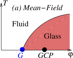
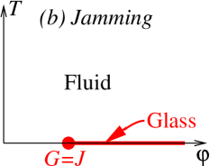
Figure 1: Sketch of two possible phase diagrams for harmonic spheres. (a) In mean-field replica calculations, an ideal glass transition occurs at finite temperature for $\varphi$ above that of point $G$, the ideal glass transition point for hard spheres. The pressure of the equilibrium glass diverges at larger density at Glass Close Packing ($GCP$). (b) No glass transition occurs before jamming at point $J$ at $T=0$ where the equilibrium pressure also diverges, with no glass transition occuring at finite temperature at larger density. Alternative phase diagrams such as (a) with $G=GCP$, or (b) with $G\neq J$ are in principle possible.

In a recent article tom , we studied the glassy dynamics of a model of soft repulsive particles where the glass transition occurs when either the particle volume fraction, $\varphi$, or the temperature, $T$, are varied, see Fig. 1. We have discovered the existence of activated dynamic scaling in the whole $(T,\varphi)$ plane constraining the actual functional form of the divergence, and allowing a precise location of the singularity. In particular, we found that in the limit $T\to 0$, where the particles become infinitely hard, a dynamic singularity seems to occur at a well-defined critical packing fraction, $\varphi_{0}$. We called ‘point $G$’ the location of this special glass point in the phase diagram shown in Fig. 1.

Our aim in the present work is to study more precisely the nature of point $G$, extending our studies to thermodynamic observables, most notably equations of state, and to explore how point $G$ fits within existing theoretical frameworks. By simultaneously studying hard and compressible particles, we are again able to put severe constraints on the nature of the dynamic divergence at point $G$. The picture which is most consistent with our data relies on the existence of a hard sphere glass phase above $\varphi_{0}$. It remains possible that the ideal glass transition reported here is eventually avoided when a much larger set of data becomes available, but we show that theories where a transition is absent describe the data rather poorly.

We first introduce the theoretical background guiding our analysis (Sec. II). We then define the numerical models (Sec. III), and successively analyze dynamic (Sec. IV) and thermodynamic (Sec. V) behaviour at thermal equilibrium, before exploring non-equilibrium glassy states (Sec. VI).

II Ideal glasses and jammed states

In this section we introduce theoretical ideas, tools and predictions needed to analyze the numerical results presented below.

II.1 Useful analogies for hard and soft particles

It is useful to draw more precise analogies between the glass transition observed in thermal glasses and in hard spheres. In thermal glasses, the natural control parameter is the temperature, $T$, and observables such a equilibrium relaxation times, $\tau_{\alpha}(T)$, and the energy density, $e(T)$, are measured. In the following, we shall measure relaxation times by studying the time decay of the self-part of the intermediate scattering function,

$$F_{s}(q,t)=\frac{1}{N}\left\langle\sum_{j=1}^{N}e^{i{\bf q}\cdot({\bf r}_{j}(t)-{\bf r}_{j}(0))}\right\rangle,$$ (1)

where ${\bf r}_{j}(t)$ represents the position of particle $j$ at time $t$ in a system composed of $N$ particles. The brackets represent an ensemble average at thermal equilibrium. In practice we define $F_{s}(q,\tau_{\alpha})=1/e$ for a fixed wavevector $q$, corresponding roughly to the first peak of the static structure factor and detecting particle motion typically over the interparticle distance. For isotropic pairwise interactions defined by the potential $V(r)$, the energy density reads

$$e=\frac{1}{N}\left\langle\sum_{i=1}^{N}\sum_{j>i}V(|{\bf r}_{i}-{\bf r}_{j}|)\right\rangle.$$ (2)

In hard sphere systems, the natural control parameter is the volume fraction,

$$\varphi=\rho\pi\sigma^{3}/6,$$ (3)

for particles of diameter $\sigma$ and a number density $\rho=N/V$, where $V$ is the volume of the sample. The equation of state of the hard sphere system is then measured by defining the reduced pressure,

$$Z(\varphi)=\frac{P}{\rho k_{B}T},$$ (4)

where $k_{B}$ is the Boltzmann constant, and $P$ the pressure. In numerical work, the pressure can be measured from the Virial,

$$Z=1-\frac{1}{3Nk_{B}T}\left\langle\sum_{i=1}^{N}\sum_{j>i}w(|{\bf r}_{i}-{\bf r}_{j}|)\right\rangle,$$ (5)

where $w(r)=rV^{\prime}(r)$. For the hard sphere system it can conveniently be reexpressed as

$$Z(\varphi)=1+4\varphi g(\sigma^{+}),$$ (6)

where $g(r=\sigma^{+})$ is the pair correlation function measured at contact.

It is interesting to notice that the volume fraction $\varphi$ plays a role analogous to the energy density $e$ in molecular glasses, while the reduced pressure is the thermodynamic parameter analogous to temperature. Since glassiness sets in when $\varphi$ and $Z$ increase in hard spheres, and when $T$ and $e$ decrease in molecular glasses, the analogy between both system reads:

$$T\leftrightarrow\frac{1}{Z},\quad e\leftrightarrow\frac{1}{\varphi}.$$ (7)

Therefore, a finite temperature singularity in thermal glasses translates into a singularity at finite pressure in hard spheres, while the limits $T\to 0$ and $Z\to\infty$ are analogous. In both limits, indeed, no particle motion is possible.

At the dynamical level, a reference law for the relaxation time of molecular glasses is the Arrhenius law,

$$\tau_{\alpha}(T)=\tau_{\infty}\exp\left(\frac{E}{k_{B}T}\right),$$ (8)

where $\tau_{\infty}$ and $E$ are two constants with dimensions of time and energy, respectively. Deviations from Arrhenius behaviour, ‘super-Arrhenius relaxation’, are often interpreted as the signature of the non-trivial cooperative nature of glassy dynamics. This physical intuition can in fact be rigorously established using concepts drawn from linear response theory science ; JCP ; dalle . Angell has introduced the notion of ‘fragility’ to quantify these deviations angell , and suggested to represent the experimental data in an Arrhenius representation, $\log\tau_{\alpha}$ vs. $1/T$. Popular functional forms to account for deviations from Arrhenius behaviour are the Vogel-Fulcher-Tamman (VFT) law,

$$\tau_{\alpha}(T)=\tau_{\infty}\exp\left(\frac{A}{(T-T_{0})^{\delta}}\right),$$ (9)

where the exponent $\delta$ is usually taken to unity, $\delta=1$, and the Bässler law,

$$\tau_{\alpha}(T)=\tau_{\infty}\exp\left(\frac{B}{T^{\alpha}}\right),$$ (10)

where the value $\alpha=2$ can be obtained from different theoretical perspectives bassler ; east ; pnas ; nef . An obvious difference between Eqs. (9) and (10) is the introduction in the former of a special temperature $T_{0}$ where the relaxation time is predicted to diverge, and below which a true glass phase should exist. In the latter, equilibrium could in principle be maintained down to $T=0$, and no glass phase exists.

Using the dictionary in Eq. (7) we now see that these well-known expressions for thermal glasses translate into relations between $\tau_{\alpha}$ and $Z$. Thus the simplest dynamic law for hard sphere, analogous to Arrhenius behaviour, reads

$$\tau_{\alpha}(\varphi)=\tau_{\infty}\exp[cZ(\varphi)],$$ (11)

where $c$ is an adimensional constant. Just as the Arrhenius law stems from considering relaxation in a liquid arising from a thermally activated local relaxation over a fixed energy barrier, Eq. (11) describes a relaxation arising from local fluctuations of the volume, which justifies fully our analogy between $T$ and $1/Z$. This idea is made more precise in free volume approaches, see Sec. II.3 below.

The VFT and Bässler expression respectively become

$$\tau_{\alpha}(\varphi)=\tau_{\infty}\exp\left(\frac{A}{[Z_{0}-Z(\varphi)]^{\delta}}\right),$$ (12)

and

$$\tau_{\alpha}(\varphi)=\tau_{\infty}\exp[BZ^{\alpha}(\varphi)].$$ (13)

However, since the experimental control parameter is the volume fraction $\varphi$ while $Z$ is often hard to access experimentally, these expressions are usually recast in terms of relations between $\tau_{\alpha}$ and $\varphi$. This can be confusing since the equivalence between soft and hard particles is then easily lost, as it depends on the explicit behaviour of the equilibrium equation of state, $Z=Z(\varphi)$. Fitting formula using $Z$ or $\varphi$ can only take mathematically equivalent forms when the pressure is finite at the volume fraction where $\tau_{\alpha}$ diverges, if it exists. A well-known example is the algebraic power laws predicted by the mode-coupling theory mct for molecular glasses,

$$\tau_{\alpha}(T)\sim(T-T_{\rm MCT})^{-\gamma},$$ (14)

and for hard spheres,

$$\tau_{\alpha}(\varphi)\sim(\varphi_{\rm MCT}-\varphi)^{-\gamma}.$$ (15)

Alternatively, an instance where the mathematical equivalence is clearly lost arises if there exists a ‘jamming’ density $\varphi^{\star}$ where $Z(\varphi)$ diverges, $Z\sim(\varphi^{\star}-\varphi)^{-1}$, because then an ‘Arrhenius’ behaviour in $Z$ as in Eq. (11) becomes similar to a ‘super-Arrhenius’ VFT form when the variable $\varphi$ is used instead. Similarly, strong and fragile molecular glass-forming materials would look alike if the energy density were used instead of the temperature, since both types of system could for instance behave as $\tau_{\alpha}\sim\exp(c/(e-e_{0}))$.

This example shows that the fragility of hard sphere systems should be evaluated by adapting the Angell plot to the pressure variable and by plotting $\log\tau_{\alpha}$ vs. $Z$, emphasizing possible deviations from the straight line corresponding to the reference law (11) sear . Note that in a recent experimental work, the Angell plot was adapted to soft colloids using $\varphi$ as an abscissa, instead of the pressure johan . The above considerations suggest that it would be very interesting to reanalyze the behaviour of these soft colloids along the lines suggested above in order to discuss possible changes of ‘fragility’.

II.2 Ideal glass transition

The above expressions for the relaxation time in thermal and hard sphere glasses can be justified from several theoretical approaches. We shall describe those theoretical frameworks which make specific predictions for both hard and soft sphere systems, and are therefore relevant to the present work.

A finite temperature/pressure dynamic singularity as in Eqs. (9) and (12) and a true glass phase exist in the context of random first order transitions KTW ; FZ . In the fluid phase before the transition, the dynamics is dominated by the existence of a large number of metastable states, allowing the definition of a finite configurational entropy. The dynamic transition coincides with the point where the configurational entropy of the fluid vanishes, and the transition is accompanied by a jump in the specific heat (for thermal glasses) or in the compressibility (for hard spheres). The glass phase is characterized by a vanishing configurational entropy, and the structure of phase space is that of a system with one-step level of replica symmetry breaking.

The existence of an ‘ideal’ glass transition is an exact result for a number of many-body interacting models defined in mean-field geometries, but remains a conjecture for three-dimensional realistic particle models. Interestingly, it is possible to turn this conjecture into a basis for actual microscopic, but approximate, calculations of the location of the glass transition and the structure of the glass phase remi ; mp . These approximations have been applied to fluids of hard and soft particles. For hard spheres, this approach predicts the existence of a divergence of $\tau_{\alpha}$ at a finite pressure, $Z_{0}$, at a packing fraction $\varphi_{0}$ FZ ; silvio ; FZ2 . Above $\varphi_{0}$ the phase which dominates the equilibrium measure is a non-ergodic glassy phase characterized by replica symmetry breaking. The equilibrium equation of state for the glass phase diverges at a packing fraction larger than $\varphi_{0}$, called ‘Glass Close Packing’, $\varphi_{GCP}$, because it corresponds to the densest possible glass with an infinite pressure FZ . Replica calculations have not been applied to the system of compressible spheres studied below, but they would presumably yield a phase diagram as sketched in Fig. 1-(a), with a glass transition line $T_{0}(\varphi>\varphi_{0})$ emerging from point $G$ at $\varphi_{0}$. It would be interesting to study also the finite temperature fate of the jamming transition at $GCP$ from this theoretical perspective.

As mentioned in the introduction, experimental evidence relies heavily on extrapolations since equilibrium can not be achieved very close to the transition. A quite favourable experimental finding is the coincidence, with reasonable if not decisive accuracy tanaka , of the extrapolated temperatures for the vanishing of the configurational entropy and for the divergence of the relaxation time obtained in several experimental studies of molecular glass-formers. For hard particles, this coincidence seems to hold in numerical studies foffi , but the extrapolations are not unambiguous, and arguably not very convincing.

II.3 Free volume ideas

Free volume arguments are very popular in the literature of the molecular glass transition freevol , although they are easier to understand in the context of hard spheres. Free volume predictions for hard spheres exist both for the equation of state and for the dynamical behaviour. In this approach, there exists a maximal packing fraction, $\varphi^{\star}$, where the equilibrium pressure of the hard sphere fluid diverges as wood :

$$Z(\varphi)=\frac{d}{1-\varphi/\varphi^{\star}},$$ (16)

where $d$ is the dimension of space. The critical packing fraction $\varphi^{\star}$ is often called ‘random close packing’ in the literature liu , but we discuss below its meaning in more detail.

To obtain dynamical predictions, one then assumes that for $\varphi<\varphi^{\star}$ each particle possesses some amount of ‘free volume’, which can then be used to perform local relaxations. In the traditional approach, one gets the ‘Arrhenius’ prediction in Eq. (11) predicting that $\tau_{\alpha}$ diverges at $\varphi^{\star}$ as

$$\tau_{\alpha}\sim\exp(cZ)\sim\exp[cd\varphi^{\star}/(\varphi^{\star}-\varphi)].$$ (17)

In this approach, $Z$ and $\tau_{\alpha}$ diverge together at the packing fraction $\varphi^{\star}$, in contrast with the ideal glass transition scenario.

Using Eq. (7), we remark that these free volume predictions are then the direct analog of the Arrhenius behaviour for thermal glasses, and should serve as a reference basis to analyze hard sphere data, the analog of ‘strong’ behaviour for thermal glasses. Physically, it indeed makes sense that the divergence in $Z$ should be accompanied by a divergence of $\tau_{\alpha}$ since no relaxation is possible when all particles touch each other, just as no relaxation occurs at $T=0$ for molecular glasses. The free volume scenario was very recently revisited in Ref. ohern , where $\varphi^{\star}$ was given a specific interpretation in terms of the jamming transition occuring at point $J$ pointJ in the phase diagram of Fig. 1-(b), predicting that $\varphi^{\star}=\varphi_{J}$. We discuss the physical meaning of $\varphi_{J}$ further below.

In recent work, Schweizer and coworkers have developed a statistical approach to describe the dynamics of hard spheres at large density ken . They obtain a self-consistent equation of motion for the dynamics of a tracer particle which they can solve either numerically, or, in some limit, analytically. In the latter case, they predict in particular a Bässler law as in Eq. (13) with $\alpha=2$. They assume further that the pressure diverges at random close packing as in Eq. (16), producing therefore the prediction of a non-trivial ‘fragile’ behaviour for hard spheres, namely

$$\tau_{\alpha}\sim\exp(BZ^{2})\sim\exp[Bd(\varphi^{\star})^{2}/(\varphi^{\star}-\varphi)^{2}].$$ (18)

Applying this body of ideas to a system of compressible spheres, we obtain the phase diagram sketched in Fig. 1-(b). Here, the hard sphere system is ergodic up to the maximal volume fraction where the equilibrium pressure diverges and the system jams, and no ideal glass transition occurs. At finite temperature, dynamic arrest only occurs in the limit where $T\to 0$ and a true glass phase never exists at finite temperature. This phase diagram is consistent with the physical idea that no glass transition can occur for thermal glasses at any finite temperature, because it is always possible to perform ‘local’ relaxations at a finite energy cost. Equivalently for hard spheres, one states that as long as some amount of free volume is available to each particle, it is possible to relax by appropriately displacing a finite set of particles. This simple argument, which can be made more formal osada , provides evidence that the self-diffusion constant for hard spheres does not vanish at finite pressure, but it says nothing about collective relaxation timescales, which can still diverge. Using (with no justification) this argument against collective freezing, one would conclude that the glass phase only exists along the $T=0$ line, as in Fig. 1-(b). Note that self and collective relaxations often yield similar results, suggesting that the formal argument in Ref. osada is not very useful for accessible timescales.

One could easily imagine scenarios intermediate between the two sketches in Fig. 1. For instance, it is sometimes stated that no glass transition can occur for thermal glasses at any finite temperature, but that hard spheres are somewhat different because of the hard constraint imposed by the potential proca . In that case, a glass phase would never exist at finite temperature, but the glass line at $T=0$ could extend down to a low-density limit occuring at a finite pressure, so that $G\neq J$. Note however that since the proof presented in Ref. proca applies to finite size systems, $N<\infty$, it does not directly contradict the existence of an equilibrium phase transition in the thermodynamic limit $N\to\infty$, as sketched in Fig. 1-(a).

The final alternative is of course the absence of a glass of hard spheres before jamming along the $T=0$ line, together with a glass transition line emerging from random close packing $T_{0}(\varphi\to\varphi^{\star})=0$. This last scenario would actually be consistent with free volume models developed for both hard and soft particles which does predict a VFT divergence at finite temperature for molecular glass-formers where the amount of ‘free volume’ disappears grest , but no such glass transition in the case of hard spheres where free volume is available up to infinite pressure.

II.4 Jamming transitions and random close packing

The glass transition described above locates state points where ergodicity is lost. For assemblies of spherical particles, another transition occurs at large density which can be defined in purely geometric terms, without invoking thermal equilibrium or ergodicity pointJ ; torquato . This jamming transition is closely related to the notion of random close packing, very widely discussed experimentally in the context of granular materials rmpgrains .

Granular experiments provide the simplest description of a jamming transition for hard particles. Due to gravity, a disordered assembly of grains will settle in the bottom of a container until contact constraints prevent any further displacements. The simplest question that can be asked is: what is the volume fraction occupied by the grains in this jammed state? Turning to frictionless spheres without gravity, the problem is therefore to produce assemblies of particles that can not be compressed further without allowing overlaps between particles pointJ ; torquato2 ; roux ; donev . These states are therefore infinite pressure hard sphere configurations. Note that the reverse is not true, because not all infinite pressure state are jammed donev .

Since several models for the dynamics of hard spheres predict that $\tau_{\alpha}$ and $Z$ diverge together at the same density, it is very natural to conjecture that glass and jamming transitions may be two facets of the same transition liunagel , which could therefore be explained in purely geometric terms matthieu . In that case, random close packing would correspond to the diverging point in the equilibrium equation of state for hard spheres, and would in effect control the glassy dynamics of colloidal particles.

The situation gets more complicated if an ideal glass transition occurs FZ ; jorge1 ; jorge2 because the equilibrium pressure does not diverge at the density where ergodicity is lost, and so jamming and glass transitions are decoupled, as sketched in Fig. 1-(a). In that case, the energy/volume fraction analogy in Eq. (7) suggests that finding the glass close packing density is equivalent to finding the energy of the ground state in a disordered system with a complex energy landscape jorge1 . This is likely a computionally hard problem. This suggests that any ‘physical’ algorithm used to produce $T=0$ or $Z=\infty$ states will end up in configurations that have an energy larger than the true ground state (in thermal glasses), or that will jam at a density smaller than the glass close packed state (in hard spheres), because they will remain trapped within the metastable states that are responsible for the glassy behaviour at low temperature/large density.

A final complication is the existence for both hard and soft particles of a first order transition towards a crystalline structure, which is ignored in the above-mentioned approaches. The existence of the crystal phase might render the fluid metastable, and crystallization can indeed occur during experiments or simulations for systems with low glass-forming ability. It is however easy to bypass crystallization in experiments for a large number of molecular systems, and for hard spheres using a sufficient amount of size polydispersity. If crystallization does not occur (which can be checked by monitoring the structure of the fluid), it is then possible to study the metastable fluid phase at ‘thermal equilibrium’, and it is the situation usually considered by theoretical approaches to the glass transition. In that case, one applies concepts from equilibrium thermodynamics to study the system in a reduced part of his phase space corresponding to metastable disordered states, the crystal region being excluded.

In the same vein, if jamming is studied by driving hard sphere configurations out of equilibrium using specific ‘physical’ algorithms for compressions, then again crystallization is not a critical issue for sufficient polydispersity. However, it should be kept in mind that a large number of crystalline and polycrystalline configurations can be built over a broad range of densities encompassing the putative glass phase, for instance by artificially mixing crystalline and fluid phases mixture . The existence of the crystal thus makes the definition of a unique ground state for thermal glasses, or the maximum packing fraction for hard spheres ‘ill-defined’ torquato , because these concepts are not made in reference to thermal equilibrium. Below, we shall study jamming transitions specifically designing algorithms for which crystallization and demixing are under controll.

To make this argument useful to analyze the (im)possibility of an equilibrium glass transition mixture , one should additionally show that nucleation of these ordered states from the disordered metastable fluid is indeed possible at thermal equilibrium. Even then, if nucleation barriers happen to be extremely large, then the glass transition might indeed be cutoff at extremely large relaxation timescales by nucleating the crystal phase rather than undergoing an ideal glass transition, but the argument is thus not necessarily useful for experimentally accessible timescales.

III Models for hard and soft particles

We have explored the equilibrium behaviour and glassy states in two numerical models for hard and soft repulsive spheres, which we now introduce.

III.1 Hard spheres

We use a standard Monte Carlo algorithm allen to study numerically a 50:50 binary mixture of hard spheres with diameters $\sigma$ and $1.4\sigma$, known to efficiently prevent crystallization pointJ . We work in a three dimensional space with periodic boundary conditions, and mainly use $N=1000$ particles when studying thermal equilibrium. No noticeable finite size effects were found in runs with $N=8000$ particles performed for selected state points. We have detected no sign of crystallization or demixing between large and small particles in all our simulations, some of which having run for more than $10^{10}$ Monte Carlo steps.

In an elementary move, a particle is chosen at random and assigned a random displacement drawn within a cubic box of linear size $0.1\sigma$ centered around the origin. The move is accepted if the hard sphere constraint remains satisfied. One Monte Carlo step corresponds to $N$ such attempts. Comparison of Monte Carlo dynamics with more standard Molecular Dynamics simulations of glass-forming liquids have provided evidence that slow relaxation in dense fluids is insensitive to the choice of a microscopic dynamics MC1 ; MC2 . This is by no means a trivial result, as both types of dynamics could in principle yield widely different results for the dynamic behaviour, especially in those cases where collective particle motions are believed to play an important role.

We have also performed non-equilibrium compressions to explore glassy states at large volume fraction. In that case we have systematically used two system sizes, $N=1000$ and $N=8000$, and the reported data for compressions are those for the larger system, although they are statistically indistinguishable from those obtained for the smaller system. To perform a compression, we use the following procedure. We start from an equilibrated hard sphere fluid configuration at a given $\varphi$. We then perform an instantaneous compression of the simulation box, which produces overlaps between particles, which are removed using the above Monte Carlo algorithm. As soon as all overlaps have disappeared, we perform the next compression of the system. We adjust the compression rate to maintain the number of overlaps after each compression below a constant number, $0.025N$. When density gets large, it becomes difficult to remove all overlaps and we stop the compression when at least one overlap has survived after $10^{5}$ Monte Carlo steps. For these non-equilibrium compressions, we have no insurance that Monte Carlo and Molecular Dynamics yield comparable results. This is not crucial for our purposes because we do not wish to perform dynamic measurements at large volume fraction.

III.2 Harmonic spheres

We use Molecular Dynamics simulations allen to study a system composed of compressible particles durian ; pointJ interacting through a pair-wise potential: $V(r_{ij})=\epsilon(1-r_{ij}/\sigma_{ij})^{2}$ for $r_{ij}<\sigma_{ij}$, $V(r_{ij})=0$ otherwise. The interparticle distance is $r_{ij}=|{\bf r}_{i}-{\bf r}_{j}|$ and $\sigma_{ij}=(\sigma_{i}+\sigma_{j})/2$, where ${\bf r}_{i}$ and $\sigma_{i}$ are the position and diameter of particle $i$, respectively. We shall use the term ‘harmonic spheres’ for this system because the repulsive force between spheres is linear in their overlap. We use system sizes between 500 and 8000 particles, and report the results obtained for $N=1000$, for which no finite size effects are detected, within numerical accuracy.

We prevent crystallisation by using the same 50:50 binary mixture of spheres of diameter ratio $1.4$ as used in the hard sphere case. Up to volume fraction $\varphi=0.846$ we detect no sign of crystallization at all studied temperatures; at and above $\varphi=0.924$ there was evidence of incipient crystallization at the lowest temperatures tom . However, these crystallization effects occur well away from the region of interest around point $G$ in the regime $\varphi=0.55-0.75$.

We use $\epsilon$ as the energy unit, and $\sqrt{\sigma_{2}^{2}/\epsilon}$ as time unit, with masses set to unity. All dynamical results are obtained at thermal equilibrium, which has been carefully controlled. When temperature is low and density is large, we are not able to thermalize. Crystallization and equilibrium issues determine the boundaries of the region of investigated state points shown in Fig. 2.

Finally we have performed exploration of glassy states of hard spheres using the compressible sphere system as follows. We start from an equilibrated configuration of harmonic spheres at a given state point $(\varphi,T)$. We then rapidly cool the system at constant density down to $T\to 0$ using Molecular Dynamics. We track pressure and energy during compression and obtain valid hard sphere configurations at $T=0$ when energy vanishes and $Z$ remains finite and independent of $T$ at sufficiently low temperatures. It is equal to the value of the pressure for the corresponding hard sphere system.

Figure 2: Phase diagram for harmonic spheres. Open symbols represent the investigated state points. The location of glass lines obtained by fitting to known functional form (MCT, VFT), and using activated scaling (22) are shown, while the ‘super-arrrhenius’ line corresponds to volume fractions where $\tau_{\alpha}(\varphi,T)$ increases faster than an Arrhenius law when $T$ is reduced at constant $\varphi$.

IV Evidence for a dynamic singularity for hard spheres

In Refs. luca ; lucalong we analyzed in detail the volume fraction dependence of the relaxation time for hard spheres, while Ref. tom contains a discussion of the interplay between density and temperature for harmonic spheres. Thus, in this section, we summarize the main conclusions drawn in these papers, and complement them by further analysis of these dynamic measurements.

IV.1 Fitting to known functional forms

For both hard and harmonic spheres, we find that algebraic divergences as predicted by mode-coupling theory only hold over a restricted time window of about 2 to 3 decades in the regime comprising the onset of glassy dynamics. This is consistent with findings in other systems mct . First, fitting the relaxation time $\tau_{\alpha}(\varphi)$ for hard spheres to Eq. (15) yields a mode-coupling singularity at $\varphi_{\rm MCT}\approx 0.592$ with a critical exponent $\gamma\approx 2.6$, as reported in Ref. luca . This is consistent with previous analysis of hard sphere systems szamel ; puertas .

Second, for harmonic spheres, we fitted the temperature evolution of $\tau_{\alpha}(\varphi,T)$ at constant $\varphi$ between $\varphi=0.61$ and $\varphi=0.924$ to Eq. (14). We thus obtain a mode-coupling transition line, $T_{\rm MCT}(\varphi)$, as shown in Fig. 2. Our data are consistent with a fitted MCT temperature which vanishes rapidly as $\varphi$ decreases towards $\varphi_{\rm MCT}$, although it is difficult to obtain an accurate determination of $T_{\rm MCT}$ very close to $\varphi_{\rm MCT}$. We find also that the critical exponent $\gamma$ in Eq. (14) has a strong volume fraction dependence, increasing from $\gamma\approx 2.8$ for $\varphi=0.612$ to a value $\gamma\approx 5.3$ for $\varphi=0.8$ and above. Although the algebraic divergence predicted by MCT is eventually avoided, as we shall describe shortly, it would be very interesting to analyze the dynamic behaviour of the harmonic sphere system using mode-coupling theory: does theory reproduce the strong density dependence of the critical exponent, and does it predict specific scaling properties in the vicinity of the hard sphere point at $T=0$ and $\varphi=\varphi_{\rm MCT}$?

Since deviations from the algebraic divergence predicted by MCT are observed at low enough temperatures, we repeated our data analysis using standard empirical approaches. First, we have fitted our data for hard spheres using a VFT form,

$$\tau_{\alpha}(\varphi)\sim\exp\left[\frac{A}{(\varphi_{0}-\varphi)^{\delta}}\right],$$ (19)

by analogy with Eq. (9). Imposing the standard value $\delta=1$, one locates a critical volume fraction at $\varphi_{\rm VFT}\equiv\varphi_{0}(\delta=1)\approx 0.615$. However, using $\delta$ as an additional fitting parameter, a slightly better fit is obtained for $\delta\approx 2.2$ from which a larger critical packing fraction, $\varphi_{0}(\delta=2.2)\approx 0.635$, is estimated. Remarkably, similar conclusions hold for experiments performed on colloidal hard spheres luca ; lucalong .

We have then fitted our finite temperature data for harmonic spheres to the VFT form in Eq. (9), imposing an exponent $\delta=1$ at all densities. We find that such a fit can describe our data at all volume fractions rather well for $\varphi>0.636$, and report the VFT glass line deduced from this fitting procedure in Fig. 2. Again it becomes difficult to obtain accurate determination of the VFT temperature as $\varphi$ decreases, but the extrapolation of the VFT line is nevertheless in good agreement with the hard sphere result $\varphi_{\rm VFT}\approx 0.615$.

An interesting outcome of the VFT fitting procedure is the density dependence obtained for the fitting parameter $A$ in Eq. (9). For $\delta=1$, it is convenient to define the parameter $D\equiv AT_{0}$, which serves as an experimental tool to quantify the fragility of supercooled liquids angell . We find that $D$ varies strongly with $\varphi$ and changes from $D\approx 55$ for $\varphi=0.636$ down to $D\approx 8$ for $\varphi>0.80$. In experimental investigations of the dynamics of supercooled liquids angell ; tanaka , $D$ is found to decrease similarly from $D\approx 60$ for SiO₂, a strong glass-forming material, down to $D\approx 30$ for liquids of intermediate fragilities such as glycerol or ZnCl₂, and to $D\approx 10$ for fragile liquids such as orthoterphenyl (the fit to a VFT form is obviously more ambiguous for strong glass-forming materials with nearly Arrhenius behaviour). Thus, we find that the system of harmonic spheres displays a variation in kinetic fragility which encompasses the range observed in experiments, a central claim made in Ref. tom , which is confirmed by the present analysis.

Both MCT and VFT fitting formula contain a divergence at a critical temperature, corresponding to the phase diagram sketched in Fig. 1-(a). However, to explore the possibility of a $T=0$ glass line at large density, as sketched in Fig. 1-(b), we have also fitted our data to a generalized Bässler form, as in Eq. (10), using $B$ and $\alpha$ as free fitting parameters for each volume fraction. We find that Eq. (10) also describes our data rather well, but we must use an exponent $\alpha$ which increases from 1 near $\varphi\approx 0.63$ up to $\alpha\approx 3.7$ at $\varphi=0.736$, while $\alpha=2$ is traditionnally preferred in supercooled liquids bassler ; fit3 . The range of density where $\alpha>1$ delimits the density region where ‘super-Arrhenius’ behaviour is observed, and is indicated with a dashed line in Fig. 2.

Therefore, we conclude cautiously that fitting our data to known functional forms shows that above $\varphi\approx 0.63$, the dynamics at constant $\varphi$ slows down with $T$ faster than an Arrhenius law, and exhibits dynamics typical of fragile glass-forming liquids, with a fragility increasing dramatically with $\varphi$. This fragility increase is accompanied by a large variation of the MCT critical exponent $\gamma$, of the VFT fitting parameter $D$, and the exponent $\alpha$ in Eq. (10), but these fitting procedures leave open the location of the divergence of $\tau_{\alpha}$, since both finite temperature and singularity-free fitting formula can be used to describe our data. Similarly, the activated form in Eq. (19) is clearly favoured by our hard sphere data, possibly with a non-trivial exponent $\delta>1$, but the location of $\varphi_{0}$ has to be extrapolated from the analysis of much smaller volume fractions, and must be discussed with caution.

IV.2 Activated scaling near point $G$

The weakness of the above analysis was mentioned in the introductory lines of this article. When independently fitting a single data set obtained by changing a single control parameter, the range of timescales covered by simulations (and experiments!) is usually too small to discrimate between very different fitting formula.

In Ref. tom we suggested to apply ideas from dynamic scaling to the data obtained in the whole $(\varphi,T)$ plane of harmonic spheres to gather more precise information on the phase diagram, and in particular the location of the dynamic singularity at point $G$. To the best of our knowledge, such an analysis using two control parameters has no counterpart in the glass transition literature.

Our main aim is to determine the location $\varphi_{0}$ of point $G$ along the $T=0$ hard sphere axis starting from the following qualitative considerations about the harmonic sphere system. For $\varphi<\varphi_{0}$, the dynamics slows down when $T$ decreases, but the relaxation time saturates in the limit $T\to 0$ to a finite value corresponding to the hard sphere fluid. For $\varphi>\varphi_{0}$, however, the relaxation time should extrapolate to infinity in this limit, by definition of $\varphi_{0}$. These two regimes are obviously delimited by $\varphi=\varphi_{0}$, where the system, like Buridan’s ass, ‘hesitates’ forever between these two regimes. These three different situations are all included in the following scaling form tom :

$$\tau_{\alpha}(\varphi,T)\sim\exp\left[\frac{A}{|\varphi_{0}-\varphi|^{\delta}}F_{\pm}\left(\frac{|\varphi_{0}-\varphi|^{2/\mu}}{T}\right)\right].$$ (20)

In this expression, $F_{\pm}(x)$ are scaling functions applying to volume fractions above and below $\varphi_{0}$, respectively. We expect therefore that $F_{-}(x\to\infty)\to 1$ to recover the hard sphere fluid limit, Eq. (19), when $T\to 0$ and $\varphi<\varphi_{0}$. Similarly, $F_{+}(x\to\infty)\to\infty$, for $\varphi>\varphi_{0}$. Moreover, continuity of $\tau_{\alpha}$ at finite $T$ when crossing $\varphi=\varphi_{0}$ implies a common limit for both scaling functions in the $x\to 0$ limit: $F_{-}(x\to 0)\sim F_{+}(x\to 0)\sim x^{\delta\mu/2}$, so that $\tau_{\alpha}(\varphi=\varphi_{0},T)\sim\exp(A/T^{\delta\mu/2})$.

Dynamic scaling was recently observed for athermal jamming transitions teitel ; hatano , but the nature of the hard sphere divergence (algebraic instead of exponential) was qualitatively different from Eq. (20), and the critical density appearing in the scaling formula also had a different nature, since these data were not collected at thermal equilibrium.

Figure 3: Activated dynamic scaling of relaxation timescales for $\varphi\in[0.567,0.736]$. The data for $\varphi<\varphi_{0}$ and $\varphi>\varphi_{0}$ collapse on two distinct branches, as described by Eq. (20). Times are rescaled by $1/\sqrt{T}$ so that the $T\to 0$ limit coincides with hard spheres thermalized at $T=1$. The errorbars describe the range of values for which acceptable data collapse is obtained; $\mu=1.3$ is fixed using potential energy considerations.

Using Eq. (20), data at all temperatures $T$, and for volume fractions in the range $\varphi\in[0.567,0.736]$ can be collapsed onto the two expected scaling branches and the best data collapse is obtained for $\varphi_{0}=0.635$, $\delta=2.2$ and $\mu=1.3$. This is shown in Fig. 3, which reproduces the data collapse presented in Ref. tom . Remarkably, while the exponent $\delta$ is not very much constrained by the hard sphere data alone, a value below $\delta\approx 2$ cannot be used if data collapse is sought for harmonic spheres at finite temperatures. Fixing $\delta$ near 2 thus allows us to estimate $\varphi_{0}$ is a much more precise manner:

$$\varphi_{0}=0.635\pm 0.005,$$ (21)

where the errorbars refer to the range of volume fractions for which acceptable data collapse is obtained.

The value of the exponent $\mu$ and the form of the scaling variable in Eq. (20) were discussed in terms of an effective hard sphere radius in Ref. tom , and the consequences on the strong volume fraction dependence of the glass fragility explored in some detail.

While the location of point $G$ is well established by the scaling analysis suggested by Eq. (20), the nature of the phase diagram for $\varphi>\varphi_{0}$ is not completely determined since it depends on the specific form of the scaling function $F_{+}(x)$ for large values of its argument. If $F_{+}(x)$ diverges at a finite value $x_{0}$, say $F_{+}(x)=x^{\mu\delta/2}/(x_{0}^{\mu/2}-x^{\mu/2})^{\delta}$, then Eq. (20) would yield a glass line of the form

$$T_{0}(\varphi)\sim(\varphi-\varphi_{0})^{2/\mu},$$ (22)

which is shown as a full line in Fig. 2. However, we checked that our data along the $F_{+}$ branch can also be described using a non-diverging form, $F_{+}(x)=x^{\mu\delta/2}(1+bx^{\beta})$, which would be consistent with a $T=0$ glass line above $\varphi_{0}$ together with the Bässler form in Eq. (10) with a density dependent effective exponent $\alpha$. Therefore, we conclude that our scaling analysis leaves open the existence of a finite temperature singularity above $\varphi_{0}$.

We emphasize that our conclusion that the equilibrium relaxation times for hard spheres diverge at the volume fraction (21) relies on a demanding scaling analysis of a large set of data in the $(\varphi,T)$ phase diagram of harmonic spheres, combined with the analysis of the $T=0$ hard sphere axis over seven decades of relaxation times. However, as is unavoidable in this field, we should not exclude that a different dynamic regime can be entered when relaxation timescales beyond reach of our numerical capabilities are added to the analysis, thereby asymptotically changing the overall picture presented in this work. If so, however, this putative new regime would be experimentally irrelevant for colloidal particles luca ; lucalong .

V Equilibrium pressure data

The above results support the existence of a non-trivial divergence of the relaxation time for hard spheres at a critical volume fraction $\varphi_{0}$. Quite generally, a divergence is expected if the equilibrium reduced pressure $Z(\varphi)$ also diverges, because no particle motion is possible in this limit, which is analogous to $T=0$ for systems with soft potentials, cf. Eq. (7). In this section, we ask whether $\varphi_{0}$ coincides with a divergence in the presssure, and whether relaxation times can be related to pressure in a direct manner.

V.1 Results for hard spheres

We first describe the equilibrium data obtained from direct equilibrium simulations of hard spheres, from which pressure is measured through Eq. (6). The results are shown as filled circles in Fig. 4 from very low volume fractions where $Z\approx 1$ up to the largest volume fraction for which equilibrium could be reached, $\varphi=0.597$, where $Z\approx 25.3$.

Figure 4: Equilibrium pressure for hard spheres obtained from direct Monte Carlo simulations (circles), and extended to large $\varphi$ using the scaling behaviour of the harmonic sphere system (triangles). The free volume prediction (16) is presented for three locations of the divergence: at $\varphi_{\rm VFT}=0.615$, $\varphi_{0}=0.635$, and the ‘best’ fit $\varphi^{\star}=0.672$, and none of them accurately describes the data. Instead, the BMCSL equation of state from liquid state theory describes the data very well over the entire fluid range and leave the pressure finite at $\varphi_{0}$, where the relaxation time diverges.

As recalled in Sec. II.3, free volume arguments predict a simple form for the divergence of pressure as $Z\sim(\varphi^{\star}-\varphi)^{-1}$. In Fig. 4 we attempt a description of our equilibrium pressure data for three values of $\varphi^{\star}$. We impose $\varphi^{\star}=\varphi_{\rm VFT}=0.615$, the volume fraction deduced from a VFT fit to the dynamic data, and $\varphi^{\star}=\varphi_{0}=0.635$, our best estimate for the location of point $G$. These fits are clearly inconsistent with the data, as they do not even go through any of the data points. This directly implies that the free volume prediction in Eq. (17) incorrectly represents our data. In the same vein, our pressure data are inconsistent with a free volume divergence of the equilibrium pressure at $\varphi_{0}$, and we do not know how to extrapolate $Z(\varphi)$ to obtain a diverging pressure at point $G$. Thus we conclude that point $G$ defined from the study of the equilibrium dynamics, does not seem to correspond to point $J$ defined from a pressure divergence, in contrast with a recent proposal based on a percolation approach ohern .

If we insist that Eq. (16) must describe at least the last data points obtained at large volume fraction we find that the value $\varphi^{\star}\approx 0.672$ represents the ‘best’ compromise, as shown in Fig. 16. Clearly, however, the shape of the pressure is not very well reproduced. Therefore, our results are in disagreement with those obtained in Ref. liu , where the equilibrium equation of state for hard spheres was fitted using a free volume expression. We believe that the discrepancy stems from the fact that non-equilibrium pressure data obtained in fast compressions were incorrectly mixed with equilibrium data and included into the free volume fit.

Finally, we show in Fig. 4 that the so-called Boublik, Mansoori, Carnahan, Starling and Leland equation of state (BMCSL) bmcsl1 ; bmcsl2 , which is the extension to binary mixtures of the Carnahan-Starling equation of state for monodisperse hard spheres, describes our equilibrium data very accurately over the entire fluid range up to $\varphi=0.597$. A similarly good agreement is known to occur when using the Carnahan-Starling equation of state applied to monodisperse systems hansen , up to large volume fractions. This excellent agreement is a remarkable result, since the BMCSL is a reasonable, but somewhat empirically derived, equation of state obtained from integral equations using uncontrolled approximations. An important feature of the BMCSL equation of state, in the present context, is that it is a continuous and derivable function up to very large volume fraction, and it predicts a singularity in the pressure at an unphysically large volume fraction, $\varphi=1$. Therefore, the BMCSL equation of state predicts neither a glass transition nor a jamming transition, and we cannot use it to extrapolate critical values of the volume fraction for the hard sphere system.

Figure 5: ‘Angell plot’ for hard spheres showing the pressure dependence of $\log\tau_{\alpha}$ where the ‘Arrhenius’ behaviour predicted by free volume arguments should appear as a straight line. Hard spheres instead display ‘fragile’ behaviour which is not well fitted either by a Bässler law, Eq. (13) with $\alpha=2$, but is consistent with a finite pressure singularity. Excellent fits to Eq. (12) with $(\delta=1,Z_{0}=30.2)$ and $(\delta=2,Z_{0}=34.4)$ are shown.

In Fig. 5 we present an ‘Angell plot for hard spheres’, that is, we show the pressure evolution of the logarithm of the relaxation time. In this plot, the Arrhenius behaviour Eq. (11) should appear as a straight line, suggesting a simple mechanism for the glassy dynamics of hard spheres. Clearly, the data in Fig. 5 do not follow such a simple law, and hard spheres thus behave in a non-trivial manner: they are ‘fragile’, in the precise sense defined in Sec. II.1. As discussed above, this is in contrast with free volume freevol and percolation-based ohern predictions for the dynamics of hard spheres.

We must thus turn to ‘fragile’ predictions for the behaviour of hard spheres as a function of pressure. We first test the prediction by Schweizer and coworkers ken in Eq. (18). We find that a fit of $\log\tau_{\alpha}$ with $Z^{2}$ is rather poor. In fact, a plot of $\log\tau_{\alpha}$ vs. $Z^{2}$ does not linearize the data, so the quadratic fit in Fig. 5 is somewhat arbitrary. Moreover, the fit shown in Fig. 5, obtained by focusing on the data at larger $\varphi$ yield a microscopic attempt time $\tau_{\infty}\sim 8\cdot 10^{-3}$ (in MC step units), which is physically much too small since it is more than 4 orders of magnitude smaller than the relaxation time obtained in the low density limit, $\tau_{\alpha}(\varphi\to 0)\approx 10^{2}$. We conclude therefore that the (asymptotic) expression in Eq. (18), although predicting the correct upward curvature in the Angell plot in Fig. 5, is not an accurate representation of our data. Thus, the near coincidence between the exponent $\delta\approx 2.2$ in Eq. (19) and the Bässler expression in Eq. (18) is fortuitous. In fact, using Eq. (13) leaving $\alpha$ free to take values different from 2, we find that the data are best described, at large density, using $\alpha\approx 6$, suggestive of a pressure dependence of the data which is much stronger than the one predicted by Eq. (18).

Therefore, we explore a final possibility, suggested by the pressure data in Fig. 4, of an equilibrium pressure which actually stays finite when the relaxation time diverges, as in Eq. (12). As can be seen in Fig. 5, our data are indeed well described by a finite pressure singularity, although the hard sphere data themselves are equally well fitted using $\delta=1$ or $\delta=2$, as shown in Fig. 5. This is expected since the volume fraction dependence of $\tau_{\alpha}$ for hard spheres was also well fitted by Eq. (19) with $\delta=1$ and $\delta=2$, the latter yielding a marginally better fit. To conclude with the pressure, we recall that a value close to $\delta=2$ was favoured through the analysis of the dynamic data for harmonic spheres. Therefore, our best estimate for the critical pressure $Z_{0}$ of the hard sphere system is obtained from the fit of the pressure with $\delta=2$ shown in Fig. 5 in the range $Z>10$ and yields:

$$Z_{0}\approx 34.4\pm 0.4,$$ (23)

with errorbars as given by the fitting numerical routine.

V.2 Pressure results for harmonic spheres

Just as investigating the dynamics of harmonic spheres in the vicinity of point $G$ allowed for an accurate determination of the critical density $\varphi_{0}$ for the divergence of the relaxation time for hard spheres, we can use the harmonic spheres to confirm the above finding that the equilibrium pressure of hard sphere is finite at $\varphi_{0}$, and obtain an independent determination of $Z_{0}$, which does not rely on the value of other fitting parameters.

The temperature evolution of the equilibrium pressure obtained in harmonic spheres for densities from $\varphi=0.581$ up to $\varphi=0.846$ is shown in the top panel of Fig. 6. For low density, the pressure $Z(\varphi,T)$ smoothly converges at low temperature to the pressure of the equilibrium hard sphere fluid. Indeed we find that $Z(\varphi,T\to 0)$ can be directly compared to the direct hard sphere simulations up to $\varphi\approx 0.6$. Of course, it becomes harder to get to $T\to 0$ at higher density because thermalization is too hard to achieve within our computer capabilities.

Figure 6: Top: Temperature dependence of the pressure of harmonic spheres at different volume fractions. Bottom: rescaling the pressure by the factor $Z(\varphi,T\to 0)$ collapses the data for all $\varphi$, in agreement with Eq. (25). For $\varphi>\varphi_{0}$ the fluid is no longer the thermodynamically stable phase at $T=0$; these data are shown with open symbols.

To analyze these pressure data, we wish to repeat the analysis performed for relaxation times in Sec. IV.2. We have first attempted to collapse the pressure data assuming that the equilibrium pressure of the hard sphere fluid diverges at point $G$. We thus tried to collapse our data using a critical scaling form near $\varphi_{0}$:

$$Z(\varphi,T)\sim f(\varphi)H_{\pm}\left(\frac{|\varphi_{0}-\varphi|^{2/\mu}}{T}\right),$$ (24)

which obviously has the same interpretation as in Eq. (20) above. To this end, we imposed the values for $\mu$ and $\varphi_{0}$ obtained in Sec. IV.2, and adjusted the function $f(\varphi)$ to obtain the ‘best’ collapse onto two distinct branches for $\varphi$ above and below $\varphi_{0}$. This approach failed, and we were not able to obtain any collapse using this procedure, showing that the scaling properties of $\tau_{\alpha}(\varphi,T)$ and $Z(\varphi,T)$ close to point $G$ are very different.

We then made the opposite hypothesis that pressure has a smooth behaviour for the fluid of hard spheres approaching point $G$ where it stays finite. This hypothesis implies that $Z(\varphi,T)$ is always a smooth function of temperature. In Fig. 6, we provide evidence supporting this hypothesis using the following much simpler scaling assumption:

$$Z(\varphi,T)\approx Z(\varphi,T\to 0)g(T),$$ (25)

where $g(T)$ is a simple function of temperature such that $g(T\to 0)=1$. To produce the collapse in Fig. 6, we adjusted $Z(\varphi,T\to 0)$ for each volume fraction to get the best collapse of the data. By definition, this limit also corresponds to the equilibrium pressure of the hard sphere fluid at this volume fraction.

We report the results for $Z(\varphi,T\to 0)$ in Fig. 4, where they can directly be compared with the direct measurements performed in Monte Carlo simulations of hard spheres. It is obvious that for $\varphi\lesssim 0.6$ both data sets perfectly overlap, confirming the validity of the scaling procedure described in Eq. (25) in this regime.

Interestingly, the data collapse in Fig. 6 allows us to extrapolate the $T\to 0$ behaviour of $Z(\varphi,T)$ for volume fractions at which equilibrium hard sphere simulations are no longer available. Therefore, the scaling factor $Z(\varphi,T\to 0)$ shown in Fig. 4 allows us to extend the fluid equation of state for hard spheres at larger $\varphi$. The validity of this extrapolation simply relies on the reasonable, but probably only approximately correct, hypothesis that the temperature dependence of $Z(\varphi,T)$ does not depend on $\varphi$ over the limited interval $\varphi\in[0.6,0.635]$, which is precisely the physical content of Eq. (25).

Moreover, since the equilibrium relaxation timescales diverges at $\varphi_{0}$, extrapolation of the fluid branch for $\varphi>\varphi_{0}$ cannot be performed because a glass phase is present. Equilibrium is lost either at a finite $T$ as in Fig. 1-(a), or because the $T\to 0$ limit is singular, as in Fig. 1-(b), and so the extrapolated value of the fluid pressure does not coincide with the pressure of the thermodynamically stable phase above $\varphi_{0}$.

Remarkably, the extension of the fluid branch up to $\varphi_{0}$ shown in Fig. 4 continues to follow the BMCSL equation of state. This result was not anticipated, since this equation of state is constructed to reproduce the behaviour at moderate volume fraction only. As mentioned above, the BMCSL pressure only diverges at $\varphi=1$, which is sometimes interpreted as a weakness of this theoretical approach because $\varphi=1$ is clearly physically accessible. Our results suggest the alternative interesting interpretation that the BMCSL pressure indeed represents the equation of state of the fluid up to large volume fractions, but the fluid is no longer the thermodynamically stable phase above $\varphi_{0}$—it is a glass FZ . Thus, the divergence of the BMCSL fluid equation of state at $\varphi=1$, and its behaviour above $\varphi_{0}$ are in fact irrelevant. We shall numerically explore the equation of state of the glass phase in the next section.

Finally, the pressure data obtained using the scaling behaviour of harmonic spheres provide an independent means to estimate the pressure of the hard sphere system at the critical volume fraction $\varphi_{0}$. The BMCSL equation of state, which represents the scaled data accurately up to $\varphi_{0}$ hits this critical density at the value

$$Z(\varphi=\varphi_{0})=34.4.$$ (26)

Obviously, the agreement with the independent estimate of $Z_{0}$ obtained above in Eq. (23) is excellent, and provides further confidence that the scaling behaviour in Eq. (25) can accurately be used.

To conclude this section, we have obtained solid evidence that the equilibrium pressure of the fluid of hard spheres is finite at point $G$. Thus the phase diagram sketched in Fig. 1-(b) does not hold, and a diverging pressure occuring when all particles are at contact cannot be reached at thermal equilibrium, suggesting that the glass transition at point $G$ does not also correspond to a jamming transition. In other words, we find that no jamming transition can be observed at thermal equilibrium. In the final section, we shall explore the consequences of this finding for understanding the jamming phenomenon.

VI Exploring multiple glassy states

In this final section, we leave the realm of thermal equilibrium to explore glassy states above $\varphi_{0}$, both for hard and harmonic spheres. As explained in Sec. III we shall use hard sphere compressions and harmonic sphere annealings to reach glassy hard sphere states. Our two main aims are to investigate the equation of state of glasses above $\varphi_{0}$, and the possibility to observe jamming transitions with a diverging pressure, which, we concluded in Sec. V, cannot be explored at thermal equilibrium. Since we abandon thermal equilibrium, we must carefully discuss our numerical protocols, because history now becomes part of the story comment .

VI.1 Choice of non-equilibrium protocols

To determine the equilibrium equation of state above $\varphi_{0}$, one should in principle get to volume fractions $\varphi>\varphi_{0}$ while maintaining thermal equilibrium. Since the system is non-ergodic, this is not possible in computer simulations, but can be done in theoretical calculations remi .

An intuitive numerical solution could be to compress a hard sphere system at a finite compression rate, $\Gamma$, with the hope that the limit $\Gamma\to 0$ can be reached LS1 ; LS2 . However, this solution has two immediate drawbacks. First, even changing $\Gamma$ by a few orders of magnitude, as can be done with present day computers, the system falls out of equilibrium much above $\varphi_{0}$, so that some extrapolation is again needed donev . A second problem stems from the difficulty in such a non-equilibrium path to check that the system is not undergoing some form of crystallization (or demixing for a mixture) while being compressed, in which case the system could end up in configurations that are not necessarily representative of the glass states one seeks to investigate. Since we dedicated much effort to tackle the ordering issue while studying thermal equilibrium, we must be similarly careful when studying glasses.

To circumvent the first of these difficulties, we decided to present equations of state obtained during compressions without attempting any sort of extrapolations. Doing so, we obtain pressure measurements at large density that are upper bound to the true equilibrium pressure, since non-equilibrium pressure are larger than the equilibrium ones, just as the energy of an annealed glass is larger than the equilibrium energy, recall Eq. (7). Therefore, we will not be able to investigate the nature of the thermodynamic transition at $\varphi_{0}$, and the possibility for the equilibrium compressibility to have a jump.

To prevent the exploration of partially ordered or demixed states, we start our compressions (for hard spheres) or annealing (for harmonic spheres) from configurations that were produced during our exploration of the fluid at thermal equilibrium, for which no tendency to order was detected, even in very long simulations. We then increase the volume fraction with a very fast compression rate, or decrease the temperature rapidly, as described in Sec. III. We have checked that the particles displacements during these very fast compressions are very small, typically much smaller than a particle diameter, so that our final configurations are no more ordered than the original fluid states. Therefore, those states are close in spirit to inherent structures usually studied in the context of soft potentials SW . Interestingly, we find that starting from equilibrium configurations, where relaxation was allowed, the pressure measured during compression or annealing is extremely weakly dependent on system size. We have in fact obtained undistinguishable results for $N=1000$ and $N=8000$ particles. This is in contrast with infinitely fast annealing from fully random configurations pointJ , which are very sensitive to system size.

VI.2 Multiple glasses and jamming densities

Having fixed compression and annealing rates to very large values, we are left with a single control parameter for exploring glassy states, namely the location of the initial equilibrium configuration in the $(\varphi,T)$ phase diagram, which we now vary.

Figure 7: Various pressure-volume fraction relations obtained from simulations of binary hard spheres. Equilibrium data and BMCSL line are as in Fig. 4. The non-equilibrium data from hard sphere compressions and soft spheres annealing demonstrate the existence of multiple branches, all diverging at different densities, and result from the glassy behaviour of hard spheres.

We first describe the results obtained during hard sphere compressions (along the $T=0$ axis) starting from different initial densities $\varphi_{\rm i}$ in the range $\varphi_{\rm i}\in[0.35,0.596]$. We follow the evolution of the pressure during compression using Eq. (6). In Fig. 7 we present the results obtained for $N=8000$ particles, averaged over 5 independent initial configurations, to obtain a better statistics.

As soon as the compression starts, the measured pressure deviates from the equilibrium equation of state, emphasizing that the compression rate is too fast for the system to relax to equilibrium, even when volume fraction is not very large. In the last stages of the compression at large volume fraction, the pressure increases very rapidly with $\varphi$, and appears to be diverging at some final density, $\varphi_{\rm f}$ (note that Fig. 7 now uses a logarithmic scale for the pressure). We stop our compressions when $Z\approx 10^{3}$, although we could easily continue compressing our system up to much larger pressures.

A central observation in Fig. 7 is that the compression curves have a strong dependence on $\varphi_{\rm i}$, which survives even in the $N\to\infty$ limit ($N=1000$ and 8000 already yield consistent results), showing that the system can be trapped in glassy states that explicitely depend on the preparation history. Since we have carefully controlled the protocol to avoid mixing compressions with partial ordering, these multiple equations of states result from the non-trivial glassy behaviour of the hard sphere system, and not from a competition between randomness and order.

This discussion equally applies to the terminal densities $\varphi_{\rm f}$ of these compression branches where pressure diverges. These configurations are the hard sphere analogs of the inherent structures obtained at $T=0$ in systems with soft potentials, and $1/\varphi_{\rm f}$ plays a role similar to the potential energy of inherent structures. The fact that $\varphi_{\rm f}$ has a strong dependence on $\varphi_{\rm i}$ thus corresponds to the observation that the energy of inherent structures decreases when the temperature is decreased sri1 , as already discussed in Refs. krauth ; dave in the context of hard spheres. We find that $\varphi_{\rm f}$ increases slowly from $\approx 0.642$ when $\varphi_{\rm i}$ is in the dilute regime, but it starts increasing more rapidly when $\varphi_{\rm i}$ gets larger than some ‘onset’ volume fraction, $\varphi_{\rm onset}\approx 0.56$, which marks the onset of slow dynamics for the hard sphere fluid dave . It then grows markedly up to $\varphi_{\rm f}\approx 0.662$ for the largest $\varphi_{\rm i}$ considered in this work. Thus our results suggest that glassiness alone can be responsible for the existence of a finite range of volume fractions where hard sphere configurations get jammed, and give an alternative explanation as to why the concept of random close packing is not ‘well-defined’, for which the existence of the crystalline phase is irrelevant torquato .

A final conclusion drawn from the compression curves in Fig. 7 is that the pressure at $\varphi_{0}$ for non-equilibrium compressions is finite. Since these non-equilibrium measurements represent upper bounds to the equilibrium pressure, we obtain a direct verification that the equilibrium pressure of the fluid does not diverge at $\varphi_{0}$. This observation does not involve fits or extrapolations.

Turning finally to harmonic spheres, we have found very similar results. We find that the $T\to 0$ limit of the pressure obtained in fast annealing of equilibrated configurations at finite temperature also strongly depends on the initial temperature, in full agreement with studies of inherent structures in systems with soft potentials sri1 . In Fig. 7, we present the result for the $T\to 0$ pressure obtained when choosing, for each volume fraction, an initial configuration corresponding to the lowest temperature for which thermal equilibrium had been reached (see the phase diagram in Fig. 2). The glass equation of state obtained this way is qualitatively very similar to the one obtained by fast compressions of well equilibrated hard spheres, and it diverges near $\varphi_{\rm f}\approx 0.664$.

This rather large volume fraction, $\varphi_{\rm f}=0.664$, provides two interesting perspectives. First, if one insists that thermal equilibrium can be maintained as long as pressure is finite, then one is led to conclude that a glass transition with a diverging relaxation time can only occur at least above $\varphi=0.664$. However, when analyzing our equilibrium dynamic data in Sec. IV, we were never able to obtain such a large value for the critical density $\varphi_{0}$. Second, if we use the theoretical perspective sketched in Fig. 1-(a) with the existence of a true glass phase for hard spheres, what we have obtained here is a lower bound on the location of the Glass Close Packing density, $0.664<\varphi_{GCP}$.

VII Conclusion

In this section, we summarize and discuss the main results of our numerical study.

VII.1 Summary

We studied a binary mixture of hard spheres at increasing volume fractions. We found that dynamics slows down dramatically, and were able to follow the first 7 decades of relaxation times. We showed that an algebraic power law, as predicted by mode-coupling theory, only describes a window of about 3 decades immediately after the onset of glassy dynamics near $\varphi_{\rm onset}\approx 0.56$. The dynamics is best fitted with a generalized VFT law, Eq. (19), with the best fit obtained for $\varphi_{0}\approx 0.635$ and $\delta\approx 2.2$, but fits with the traditional value $\delta=1$ diverging near $\varphi_{\rm VFT}\approx 0.615$ were acceptable.

We found that the volume fraction dependence of the equilibrium pressure was rather modest, and were not able to extrapolate these data to obtain a critical volume fraction where the pressure diverges, implying that $\tau_{\alpha}$ and $Z$ do not appear to diverge at the same volume fraction, in contrast with free volume arguments.

We suggested to build an ‘Angell plot for hard spheres’, representing the evolution of $\log\tau_{\alpha}$ vs. $Z$, parametrized by $\varphi$. In this representation, the density analog of the Arrhenius behaviour, Eq. (11), appears as a straight line. We find instead that hard spheres display a ‘fragile’ behaviour, since the pressure dependence of $\tau_{\alpha}$ is much more marked. In this representation, we could show that several theoretical predictions for the dynamic behaviour of hard spheres do not describe our data, the best description being offered by the hypothesis that dynamics diverges at a finite pressure. We estimated $Z_{0}\approx 34.4$ for the present system.

We have shown that extending these study using temperature as a second, independent control parameter, could provide an independent confirmation of these conclusions about the dynamic and thermodynamic behaviour of hard spheres. These temperature studies were moreover able to make the above statements quantitatively much more convincing. By using dynamic scaling ideas, we determined the location $\varphi_{0}$ of the divergence, and the functional form of the relaxation time with a better precision, showing in particular that the most commonly used value $\delta=1$ in Eq. (19) was incompatible with our data. For thermodynamic quantities, we discovered a much simpler scaling behaviour of the pressure, allowing to confirm that $Z$ is not divergent at the dynamic transition $\varphi_{0}$.

We have directly confirmed this statement by devising non-equilibrium paths to explore glassy states at large volume fractions, carefully dealing with crystallization and demixing issues. We have found a family of non-equilibrium equations of state in the glass phase, which can be seen as upper bounds to the true equilibrium equation of state above $\varphi_{0}$. We have shown that these multiple branches remain distinct in the thermodynamic limit, and diverge in a broad range of volume fractions between $\varphi=0.642$ and $\varphi=0.664$, where configurations get jammed.

VII.2 Discussion and open questions

Gathering the above results sheds light on the possible phase diagrams for the harmonic sphere system sketched in Fig. 1, and its $T=0$ limit where it coincides with the hard sphere system.

The best description of our data is obtained if we assume that the relaxation time in the hard sphere limit diverges at $\varphi_{0}\approx 0.635$, where the equilibrium pressure of the fluid is $Z_{0}\approx 34.4$. Although these numerical values are specific to the present binary mixture studied in this work, these results invalidate a number of theoretical approaches predicting $Z_{0}=\infty$, and more generally the idea that the dynamic arrest in hard spheres simply occurs when the interparticle distance vanishes freevol ; liu ; ohern ; ken . The only theoretical scenario where a glass transition occurs at finite pressure is the one predicted by theories and calculations based on the concept of an ideal glass transition of the random first order type KTW ; FZ ; FZ2 . So, we are led to the conclusion that our data provide strong support for this scenario in the context of hard spheres. We were not able to provide a similar evidence for the temperature behaviour of harmonic spheres above $\varphi_{0}$, and the possibility of a finite temperature glass line as in Fig. 1-(a) remains an open issue.

Since we opened the paper with ironic remarks about such sharp claims about the existence of glass transitions, let us make here a series of cautious remarks about the above statement for hard spheres. First, we repeat that our conclusions are based upon solid, but necessarily limited in range, numerical evidence. Thus, we leave open the possiblity that the picture changes when a broader range of timescales is covered. But we also insist that the range covered numerically is just as large as the range covered experimentally in colloids luca , while work in the field of molecular glasses suggest that the physics hardly changes when several decades of relaxation timescales are added. Thus, we can at least claim experimental relevance for our results.

Second, although we suggest that the nature of point $G$ is consistent with an ideal glass transition of the random first order type, its precise nature remains to be established. Theoretically, such a transition is defined by the vanishing of the configurational entropy counting the number of metastable states. Thus, it would be important to measure the configurational entropy numerically in the vicinity of point $G$. Unfortunately, only approximations to the configurational entropy can be accessed numerically, because the very concept of metastable states is not well-defined jorge3 . Another potential problematic aspect concerns the dynamical behaviour predicted within random first order theory: the exponent $\delta\approx 2.2$ in Eq. (19) is usually not the one used when analyzing experimental data in molecular glasses, and is not the one predicted in Ref. KTW , although scaling arguments BB suggest ways out of the problem that remain to be worked out. Also, since explicit replica calculations only exist in the hard sphere limit, it would certainly be worthwile to extend the computation to harmonic spheres at finite temperature. Work is in progress in this direction.

The third remark of caution stems from the existing line of research which aims at demonstrating that an ideal glass transition cannot exist in hard spheres. In Sec. II.4, we discussed why we believe published theoretical arguments do not establish the irrelevance of a concept of an ideal glass transition in hard spheres, even for the specific case considered in Ref. mixture . Numerical evidence against the existence of an ideal glass transition was also given in Ref. krauth . We stress, however, that the location of $\varphi_{0}$ in this last work was defined using algebraic laws for the relaxation time, as in Eq. (15). Using a similar description we would have (incorrectly) located $\varphi_{0}$ close to $\varphi_{\rm MCT}\approx 0.592$, where we indeed were able to show that the pressure is not singular, in agreement with Ref. krauth . Therefore, the path to disprove our conclusions about the nature and location of point $G$ is clear: one should provide numerical evidence that thermal equilibrium can be maintained for the present binary mixture with no pressure singularity for volume fractions larger than $\varphi_{0}\approx 0.635$ and pressures larger than $Z_{0}\approx 34.4$. We believe this is a hard numerical task, even when using smart algorithms dave2 .

A final suggestion for future research is the connection to jamming transitions suggested in Fig. 7. We provided direct evidence that a ‘random close packing’ density can not be provided in a unique manner, as jamming transitions can occur within a finite range of volume fractions. Our argument is different from the one presented in Ref. torquato , since it does not rely on the existence of a crystalline or ordered phase. It is, however, in good agreement with recent work using ideas from random first order theory to study jamming of hard spheres jorge1 ; jorge2 ; FZ . In future work, we shall study more precisely the final configurations obtained when pressure diverges in Fig. 7. Our conclusion that, along the metastable fluid branch, an ideal glass transition intervenes at finite pressure shows that a ‘reproducible’ jamming transition cannot be observed at thermal equilibrium. This shows also that the glass transition is likely not driven by geometric jamming, but we can tentatively use the jamming phase diagram of Ref. liunagel in the opposite direction and claim that glassiness observed in glass-forming liquids carries indeed interesting consequences for understanding jamming transitions.

- (1) Spin glasses and random fields, Ed.: A. P. Young (World Scientific, Singapore, 1998).
- (2) K. Binder and A. P. Young, Rev. Mod. Phys. 58, 801 (1986).
- (3) M. J. P. Gingras, C. V. Stager, N. P. Raju, B. D. Gaulin, J. E. Greedan, Phys. Rev. Lett. 78, 947 (1997).
- (4) Slow relaxations and nonequilibrium dynamics in condensed matter, Eds: J.-L. Barrat, J. Dalibard, M. Feigelman, J. Kurchan (Springer, Berlin, 2003).
- (5) Jamming and rheology: Constrained dynamics on microscopic and macroscopic Scales, Eds.: A. J. Liu and S. R. Nagel (Taylor and Francis, New York, 2001).
- (6) P. G. Debenedetti and F. H. Stillinger, Nature 410, 259 (2001).
- (7) T. Hecksher, A. I. Nielsen, N. B. Olsen, and J. C. Dyre, Nature Physics 4, 737 (2008).
- (8) D. Kivelson, X. Zhao, G. Tarjus, and S. Kivelson, Phys. Rev. E 53, 751 (1996).
- (9) Y. S. Elmatad, D. Chandler, and J. P. Garrahan, to be published in J. Phys. Chem. B; arXiv:0811.2450.
- (10) P. N. Pusey and W. Van Megen, Nature 320, 595 (1986).
- (11) W. van Megen, T. C. Mortensen, S. R. Williams, and J. Muller, Phys. Rev. E 58, 6073 (1998).
- (12) Z. Cheng, J. Zhu, P. M. Chaikin, S. Phan, and W. B. Russel, Phys. Rev. E 65, 041405 (2002).
- (13) G. Brambilla, D. El Masri, M. Pierno, G. Petekidis, A. B. Schofield, L. Berthier, and L. Cipelletti, Phys. Rev. Lett. 102, 085703 (2009).
- (14) L. Berthier and T. A. Witten, arXiv:0810.4405.
- (15) L. Berthier, G. Biroli, J. P. Bouchaud, L. Cipelletti, D. El Masri, D. L’Hote, F. Ladieu, and M. Pierno, Science 310, 1797 (2005).
- (16) L. Berthier, G. Biroli, J.-P. Bouchaud, W. Kob, K. Miyazaki, and D. R. Reichman, J. Chem. Phys. 126, 184503 (2007); J. Chem. Phys. 126, 184504 (2007).
- (17) C. Dalle-Ferrier, C. Thibierge, C. Alba-Simionesco, L. Berthier, G. Biroli, J.-P. Bouchaud, F. Ladieu, D. L’Hôte, and G. Tarjus, Phys. Rev. E 76, 041510 (2007).
- (18) C. A. Angell, Science 267, 1924 (1995).
- (19) H. Bässler, Phys. Rev. Lett. 58, 767 (1987).
- (20) J. Jäckle and S. Eisinger, Z. Phys. B 84, 115 (1991).
- (21) J.P. Garrahan and D. Chandler, Proc. Natl. Acad. Sci. USA 100, 9710 (2003).
- (22) L. Berthier and J.P. Garrahan, J. Phys. Chem. B 109, 3578 (2005).
- (23) W. Götze, Complex dynamics of glass-forming liquids (Oxford University Press, Oxford, 2009).
- (24) R. P. Sear, J. Chem. Phys. 113, 4732 (2000).
- (25) J. Mattsson, H. M. Wyss, A. Fernandez-Nieves, K. Miyazaki, Z. Hu, D. R. Reichman, and D. A. Weitz, submitted.
- (26) T. R. Kirkpatrick, D. Thirumalai, and P. G. Wolynes, Phys. Rev. A 40, 1045 (1989).
- (27) G. Parisi and F. Zamponi, arXiv:0802.2180.
- (28) R. Monasson, Phys. Rev. Lett. 75, 2847 (1995).
- (29) M. Mézard and G. Parisi, J. Chem. Phys. 111, 1076 (1999).
- (30) M. Cardenas, S. Franz, and G. Parisi, J. Chem. Phys. 110, 1726 (1999).
- (31) G. Parisi and F. Zamponi, J. Chem. Phys. 123, 144501 (2005).
- (32) H. Tanaka, Phys. Rev. Lett. 90, 055701 (2003).
- (33) L. Angelani and G. Foffi, J. Phys.: Condens. Matter 19, 256207 (2007).
- (34) M. H. Cohen and D. Turnbull, J. Chem. Phys. 31, 1164 (1959).
- (35) Z. W. Salsburg and W. W. Wood, J. Chem. Phys. 37, 798 (1962).
- (36) R. D. Kamien and A. J. Liu, Phys. Rev. Lett. 99, 155501 (2007).
- (37) G. Lois, J. Blawzdziewicz, and C. S. O’Hern Phys. Rev. Lett. 102, 015702 (2009).
- (38) C. S. O’Hern, S. A. Langer, A. J. Liu, and S. R. Nagel, Phys. Rev. Lett. 88 075507 (2002).
- (39) K. S. Schweizer, J. Chem. Phys. 127, 164506 (2007).
- (40) H. Osada, Probab. Theory Relat. Fields 112, 53 (1998).
- (41) J.-P. Eckmann and I. Procaccia, Phys. Rev. E 78, 011503 (2008).
- (42) M. H. Cohen and G. S. Grest, Phys. Rev. B 20, 1077 (1979).
- (43) S. Torquato, T. M. Truskett, and P. G. Debenedetti, Phys. Rev. Lett. 84, 2064 (2000).
- (44) H. M. Jaeger, S. R. Nagel, and R. P. Behringer, Rev. Mod. Phys. 68, 1259 (1996).
- (45) M. D. Rintoul and S. Torquato, J. Chem. Phys. 105, 9258 (1996).
- (46) J. N. Roux, Phys. Rev. E 61, 6802 (2000).
- (47) A. Donev, S. Torquato, and F. H. Stillinger, Phys. Rev. E 71, 011105 (2005).
- (48) A. J. Liu and S. R. Nagel, Nature 396, 21 (1998).
- (49) C. Brito and M. Wyart, Europhys. Lett. 76, 149 (2006).
- (50) F. Krzakala, and J. Kurchan, Phys. Rev. E 76, 021122 (2007).
- (51) R. Mari, F. Krzakala, and J. Kurchan, arXiv:0806.3665.
- (52) A. Donev, F. H. Stillinger, and S. Torquato, J. Chem. Phys. 127, 124509 (2007).
- (53) M. Allen and D. Tildesley, Computer Simulation of Liquids (Oxford University Press, Oxford, 1987).
- (54) L. Berthier and W. Kob, J. Phys.: Condens. Matter 19, 205130 (2007).
- (55) L. Berthier, Phys. Rev. E 76, 011507 (2007).
- (56) D. J. Durian, Phys. Rev. Lett. 75, 4780 (1995).
- (57) S. K. Kumar, G. Szamel, and J. F. Douglas, J. Chem. Phys. 124, 214501 (2006).
- (58) T. Voigtmann, A. M. Puertas, and M. Fuchs, Phys. Rev. E 70, 061506 (2004).
- (59) G. Brambilla, D. El Masri, M. Pierno, G. Petekidis, A. B. Schofield, L. Berthier, and L. Cipelletti, arXiv:0903.1933.
- (60) P. Olsson and S. Teitel, Phys. Rev. Lett. 99, 178001 (2007).
- (61) T. Hatano, J. Phys. Soc. Jpn. 77, 123002 (2008).
- (62) T. Boublik, J. Chem. Phys. 53, 471 (1970).
- (63) G. A. Mansoori, N. F. Carnahan, K. E. Starling, and T. W. Leland, J. Chem. Phys. 54, 1523 (1971).
- (64) J. P. Hansen and I. R. McDonald, Theory of Simple Liquids (Elsevier, Amsterdam, 1986).
- (65) A. Donev, S. Torquato, F. H. Stillinger, and R. Connelly, Phys. Rev. E 70, 043301 (2004).
- (66) B. D. Lubachevsky and F. H. Stillinger, J. Stat. Phys. 60, 561 (1990).
- (67) B. D. Lubachevsky, F. H. Stillinger, and E. N. Pinson, J. Stat. Phys. 64, 501 (1990).
- (68) F. H. Stillinger and T. A. Weber, Phys. Rev. A 25, 978 (1982).
- (69) S. Sastry, P. G. Debenedetti, and F. H. Stillinger, Nature 393, 554 (1998).
- (70) L. Santen and W. Krauth, Nature 405, 550 (2000).
- (71) Y. Brumer and D. R. Reichman, Phys. Rev. E 69, 041202 (2004).
- (72) Y. Brumer and D. R. Reichman, J. Phys. Chem. B 108, 6832 (2004).
- (73) G. Biroli and J. Kurchan. Phys. Rev. E 64, 016101 (2001).
- (74) J.-P. Bouchaud and G. Biroli. J. Chem. Phys. 121, 7347 (2004).
- (75) See: http://en.wikipedia.org/wiki/GoldbergVariations.