Abstract

The turbulent jets are usually described by classical velocities. The relativistic case can be treated starting from the conservation of the relativistic momentum. The two key assumptions which allow to obtain a simple expression for the relativistic trajectory and relativistic velocity are null pressure and constant density.

Adv. Studies Theor. Phys, Vol. x, 200x, no. xx, xxx - xxx

The relativistic equation of motion in

turbulent jets

L. Zaninetti

Dipartimento di Fisica Generale

Università degli Studi di Torino

via P.Giuria 1, 10125 Torino,Italy

PACS: 47.75.+f ; 47.27.-i; 47.27.wg
Keywords: Relativistic fluid dynamics ; Turbulent flows Turbulent jets

1 Introduction

The theory of turbulent jets emerging from a circular hole can be found in different books which adopt different theories foot ; landau ; goldstein ; Pope2000 or in specialized articles List1982 ; Launder1983 : in all the models the pressure , $p$, is equal to zero. The centerline velocity is always taken to be classical. This paper briefly reviews in Section 2 the simplest model of turbulent jets and then investigates in Section 3 the case of relativistic centerline velocity .

2 Classical equations

The starting point is the conservation of the momentum’s flux in a ”turbulent jet” as outlined in landau (pag. 147). The section ,$A$, is :

$$A=\pi~{}r^{2}\quad$$ (1)

where $r$ is the radius of the jet. Once $\alpha$ the opening angle , $x_{0}$ the initial position on the $x$–axis and $v_{0}$ the initial velocity are introduced, the section $A$ at position $x$ is

$$A(x)=\pi\bigl{(}{\it r_{0}}+\left(x-{\it x_{0}}\right)\tan\left((1/2)\,\alpha\right)\bigr{)}^{2}\quad.$$ (2)

The conservation of the total momentum flux states that

$$\rho v_{0}^{2}A_{0}=\rho v(x)^{2}A(x)\quad,$$ (3)

where $v(x)$ is the velocity at position $x$ and $A_{0}$ the initial section.

Due to the turbulent transfer, the density $\rho$ is the same on both the two sides of equation (3). The trajectory of the jet as a function of the time is easily deduced from equation (3)

$$x=-{\frac{-{\it x_{0}}\,\tan\left((1/2)\,\alpha\right)+{\it r_{0}}-\sqrt{{\it r_{0}}\,\left({\it r_{0}}+2\,\tan\left((1/2)\,\alpha\right){\it v_{0}}\,t\right)}}{\tan\left((1/2)\,\alpha\right)}}\quad.$$ (4)

The velocity turns out to be

$${\it v(t)}={\frac{{\it v_{0}}\,{\it r_{0}}}{\sqrt{{\it r_{0}}\,\left({\it r_{0}}+2\,\tan\left((1/2)\,\alpha\right){\it v_{0}}\,t\right)}}}\quad.$$ (5)

3 Relativistic equations

A relativistic flow on flat space time is described by the energy-momentum tensor ,$T^{\mu\nu}$,

$$T^{\mu\nu}=wu^{\mu}u^{\nu}-pg^{\mu\nu}\quad,$$ (6)

where $u^{\mu}$ is the 4-velocity , and the Greek index varies from 0 to 3 , $w$ is the enthalpy for unit volume , $p$ is the pressure and $g^{\mu\nu}$ the inverse metric of the manifold landau ; Hidalgo2005 ; Gourgoulhon2006 . The momentum conservation in the presence of velocity , $v$, along one direction states that

$$(w(\frac{v}{c})^{2}\frac{1}{1-\frac{v^{2}}{c^{2}}}+p)A=cost\quad,$$ (7)

where $A(x)$ is the considered area in the direction perpendicular to the motion. The enthalpy for unit volume is

$$w=c^{2}\rho+p\quad,$$ (8)

where $\rho$ is the density , and $c$ the light velocity. The reader may be puzzled by the $\gamma^{2}$ factor in equation (7), where $\gamma^{2}=\frac{1}{1-\frac{v^{2}}{c^{2}}}$. However it should be remembered that $w$ is not an enthalpy, but an enthalpy per unit volume: the extra $\gamma$ factor arises from ”length contraction” in the direction of motion Gourgoulhon2006 . According to the current models on classical turbulent jets we insert $p=0$ and the momentum conservation law is

$$(\rho v^{2}\frac{1}{1-\frac{v^{2}}{c^{2}}})A=cost\quad.$$ (9)

Note the similarity between the previous formula and condition (135.2) in landau concerning the shock waves : when $A$=1 they are equals. We assume that the cross section of the relativistic jet grows as

$$A(x)=\pi\times(r_{0}+\tan(\frac{\alpha}{2}))^{2}\quad,$$ (10)

with $\alpha$ , the opening angle of the jet, constant. In two sections of the jet we have :

$$\rho\,{{\it v_{0}}}^{2}\pi\,{{\it r_{0}}}^{2}{\frac{1}{1-{\frac{{{\it v_{0}}}^{2}}{{c}^{2}}}}} =$$

$$\rho\,{v}^{2}\left((\pi\,{{\it r_{0}}}^{2}+\pi\,{\it r_{0}}\,x\alpha+O\left({\alpha}^{2}\right))\right){\frac{1}{1-{\frac{{v}^{2}}{{c}^{2}}}}} ~{}\quad,$$ (11)

where $v$ is the velocity at position $x$, $v_{0}$ the velocity at $x$=0 and $c$ the light velocity.

As due to the turbulent transfer, the density $\rho$ is the same on both sides of equation (11) and the following second degree equation in $\beta=\frac{v}{c}$ is obtained:

$${{\it\beta}}^{2}{\it r_{0}}+{{\it\beta}}^{2}x\alpha-{{\it\beta}}^{2}{{\it\beta_{0}}}^{2}x\alpha-{{\it\beta_{0}}}^{2}{\it r_{0}}=0$$ (12)

where $\beta_{0}=\frac{v_{0}}{c}$. The positive solution is :

$$\beta={\frac{\sqrt{{\it r_{0}}}{\it\beta_{0}}}{\sqrt{{\it r_{0}}+x\alpha-{{\it\beta_{0}}}^{2}x\alpha}}}\quad.$$ (13)

From equation (13) it is possible to deduce the distance $x_{f}$ after which the velocity is a fraction $f$ of the initial value, $v=fv_{0}$ :

$$x_{f}=\frac{{\it r_{0}}\,\left({f}^{2}-1\right)}{\alpha\,{f}^{2}\left(-1+{{\it\beta_{0}}}^{2}\right)}\quad.$$ (14)

The trajectory of the relativistic jet as a function of the time can be deduced from equation ( 13) and is

$$\int_{0}^{x}\frac{1}{{\frac{\sqrt{{\it r_{0}}}{\it\beta_{0}}}{\sqrt{{\it r_{0}}+x\alpha-{{\it\beta_{0}}}^{2}x\alpha}}}}dx=ct\quad.$$ (15)

On integrating the equation of the trajectory is obtained

$$\frac{2}{3}\,{\frac{{{\it r_{0}}}^{3/2}-\left({\it r_{0}}+x\alpha-{{\it\beta_{0}}}^{2}x\alpha\right)^{3/2}}{\alpha\,\left(-1+{{\it\beta_{0}}}^{2}\right)\sqrt{{\it r_{0}}}{\it\beta_{0}}}}-ct=0\quad.$$ (16)

After some manipulation equation (16) becomes a cubic polynomial equation

$$\left(-3\,{\alpha}^{3}{{\it\beta_{0}}}^{2}+3\,{\alpha}^{3}{{\it\beta_{0}}}^{4}-{{\it\beta_{0}}}^{6}{\alpha}^{3}+{\alpha}^{3}\right){x}^{3}+$$

$$\left(3\,{\it r_{0}}\,{\alpha}^{2}-6\,{\it r_{0}}\,{\alpha}^{2}{{\it\beta_{0}}}^{2}+3\,{\it r_{0}}\,{{\it\beta_{0}}}^{4}{\alpha}^{2}\right){x}^{2}+$$

$$\left(-3\,{{\it r_{0}}}^{2}{{\it\beta_{0}}}^{2}\alpha+3\,{{\it r_{0}}}^{2}\alpha\right)x-$$

$$9/4\,{c}^{2}{t}^{2}{\alpha}^{2}{\it r_{0}}\,{{\it\beta_{0}}}^{6}-3\,{{\it r_{0}}}^{2}ct\alpha\,{\it\beta_{0}}+3\,{{\it r_{0}}}^{2}ct\alpha\,{{\it\beta_{0}}}^{3}-$$

$$9/4\,{c}^{2}{t}^{2}{\alpha}^{2}{\it r_{0}}\,{{\it\beta_{0}}}^{2}+9/2\,{c}^{2}{t}^{2}{\alpha}^{2}{\it r_{0}}\,{{\it\beta_{0}}}^{4}=0\quad.$$ (17)

We briefly review that in order to solve the cubic polynomial equation

$$a_{{0}}{x}^{3}+a_{{1}}{x}^{2}+a_{{2}}x+a_{{3}}=0\quad,$$ (18)

for $x$, the first step is to apply the transformation

$$x=y-\frac{1}{3}\,{\frac{a_{{1}}}{a_{{0}}}}\quad.$$ (19)

This reduces the equation to

$$y^{3}+py+q=0\quad,$$ (20)

where

$$p = \frac{1}{3}\,{\frac{3\,a_{{2}}a_{{0}}-{a_{{1}}}^{2}}{{a_{{0}}}^{2}}}$$ (21)

$$q = \frac{1}{27}\,{\frac{27\,a_{{3}}{a_{{0}}}^{2}+2\,{a_{{1}}}^{3}-9\,a_{{2}}a_{{1}}a_{{0}}}{{a_{{0}}}^{3}}}.$$ (22)

The next step is to compute the first derivative of the left hand side of equation (20) calling it $f(y)^{\prime}$

$$f(y)^{\prime}=3y^{2}+p\quad.$$ (24)

In our case $p=0$ and in the range of existence $-\infty<y<\infty$ the first derivative is always positive and equation (20) has only one root which is real , more precisely ,

$$y=\frac{1}{6}\,\sqrt[3]{-108\,{\it q}+12\,\sqrt{12\,{{\it p}}^{3}+81\,{{\it q}}^{2}}}$$

$$-2\,{\frac{{\it p}}{\sqrt[3]{-108\,{\it q}+12\,\sqrt{12\,{{\it p}}^{3}+81\,{{\it q}}^{2}}}}}\quad,$$ (25)

or equation (18) has the solution in terms of $a_{0}$,$a_{1}$,$a_{2}$ and $a_{3}$

$$x=\frac{1}{6}\,\sqrt[3]{A+12\,\sqrt{B}}$$

$$-\frac{2}{3}\,\left(3\,a_{{2}}a_{{0}}-{a_{{1}}}^{2}\right)\frac{1}{a_{0}^{2}}{\frac{1}{\sqrt[3]{A+12\,\sqrt{B}}}}$$ (26)

where

$$A=-36\,{\frac{3\,a_{{2}}a_{{0}}-{a_{{1}}}^{2}}{{a_{{0}}}^{2}}}$$

$$B=\frac{4}{9}\,{\frac{\left(3\,a_{{2}}a_{{0}}-{a_{{1}}}^{2}\right)^{3}}{{a_{{0}}}^{6}}}+9\,{\frac{\left(3\,a_{{2}}a_{{0}}-{a_{{1}}}^{2}\right)^{2}}{{a_{{0}}}^{4}}}\quad.$$

When the equation (17) is considered we have $p=0$ and therefore we have one real root which is :

$$x(t)=$$

$$\frac{1}{2}{\frac{2{\it r_{0}}-\sqrt[3]{2}\sqrt[3]{{\it r_{0}}}\left(2{\it r_{0}}+3ct\alpha{\it\beta_{0}}-3ct\alpha{{\it\beta_{0}}}^{3}\right)^{2/3}}{\alpha\left({{\it\beta_{0}}}^{2}-1\right)}}$$ . (27)

This is the law of motion of the relativistic turbulent jets and the velocity as function of the time is

$$v(t)={\frac{c{\it\beta_{0}}\sqrt[3]{{\it r_{0}}}\sqrt[3]{2}}{\sqrt[3]{2{\it r_{0}}+3ct\alpha{\it\beta_{0}}-3ct\alpha{{\it\beta_{0}}}^{3}}}}\quad.$$ (28)

Figure 1 reports the classical and relativistic behavior of the velocity as a function of the distance from the nozzle and Figure 2 the distance traveled by the jet as a function of the time.

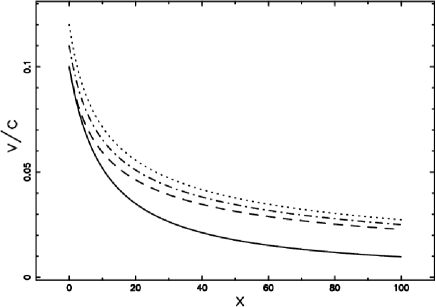
Figure 1: Velocity as function of the distance from the nozzle when $r_{0}=1$ , $x_{0}=0$, $\alpha=0.185$ and $v_{0}/c=0.1~{}(classical~{}case,~{}equation~{}(\ref{velocitac}))$ (full line ) , $v_{0}/c=\beta_{0}=0.1~{}(relativistic~{}case,~{}equation~{}(\ref{velocitar}))$ (dashed ) , $v_{0}/c=\beta_{0}=0.11~{}(relativistic~{}case,~{}equation~{}(\ref{velocitar}))$ (dot-dash-dot-dash ) and $v_{0}/c=\beta_{0}=0.12~{}(relativistic~{}case,~{}equation~{}(\ref{velocitar}))$ ( dotted ).

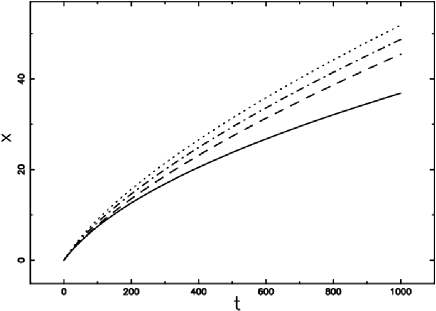
Figure 2: Distance from the nozzle as function of the time when $r_{0}=1$ , $x_{0}=0$, $\alpha=0.185$ , $c=1$ and $v_{0}/c=0.1~{}(classical~{}case,~{}equation~{}(\ref{traiettoriac}))$ (full line ), $v_{0}/c=\beta_{0}=0.1~{}(relativistic~{}case,~{}equation~{}(\ref{traiettoriarel}))$ (dashed ), $v_{0}/c=\beta_{0}=0.11~{}(relativistic~{}case,~{}equation~{}(\ref{traiettoriarel}))$ (dot-dash-dot-dash) and $v_{0}/c=\beta_{0}=0.12~{}(relativistic~{}case,~{}equation~{}\ref{traiettoriarel}))$ (dotted).

4 Conclusions

The complicate behavior of the energy tensor that describes the relativistic fluids takes a simple expression in the case of null pressure. This allows to deduce the law of motion of the relativistic turbulent jet as well the velocity behavior as function of the distance from the nozzle.

References

(1)
R. Bird, W. Stewart, E. Lightfoot, Transport Phenomena ; second
Edition, John Wiley and Sons, New York, 2002.
(2)
L. Landau, Fluid Mechanics 2nd edition, Pergamon Press, New York, 1987.
(3)
S. Goldstein, Modern Developments in Fluid Dynamics, Dover, New York,
1965.
(4)
S. B. Pope, Turbulent Flows, Cambridge University Press, Cambridge,
UK, 2000.
(5)
E. J. List, Turbulent jets and plumes, Annual Review of Fluid
Mechanics14 (1982), 189–212.
(6)
B. E. Launder, W. Rodi, The turbulent wall jet - Measurements and
modeling, Annual Review of Fluid Mechanics15 (1983), 429–459.
(7)
J. C. Hidalgo, S. Mendoza, Self-similar imploding relativistic shock
waves, Physics of Fluids17 (2005), 6101–8.
(8)
E. Gourgoulhon, An introduction to relativistic hydrodynamics, EAS
PUBL.SER.21 (2006), 43–80.