Affine transformation crossed product like
algebras and noncommutative surfaces

Abstract.

Several classes of $*$-algebras associated to the action of an affine transformation are considered, and an investigation of the interplay between the different classes of algebras is initiated. Connections are established that relate representations of $*$-algebras, geometry of algebraic surfaces, dynamics of affine transformations, graphs and algebras coming from a quantization procedure of Poisson structures. In particular, algebras related to surfaces being inverse images of fourth order polynomials (in $\mathbb{R}^{3}$) are studied in detail, and a close link between representation theory and geometric properties is established for compact as well as non-compact surfaces.

1. Introduction

The interplay between representation theory of $*$-algebras and dynamical systems or more general actions of groups or semi-groups is an expanding area of investigation deeply intertwined with origins of quantum mechanics, foundations of invariants and number theory, symmetry analysis, symplectic geometry, dynamical systems and ergodic theory and several other parts of mathematics that are fundamental for modern physics and engineering. There has been three main frameworks for investigation of such broad interplay. These frameworks are intertwining greatly in terms of mathematical ideas, constructions and goals, but developed to some extant independently in the last sixty years due to historical and other reasons. One approach is based on the systematic use of crossed product type operator algebras, that is $C^{*}$-algebras and $W^{*}$-algebras, constructed as crossed products of a ”coefficient” algebra with a group (or more generally a semi-group) acting on it. In particular, for a topological space, an algebra of continuous functions encodes properties of the space. The dynamics given by iteration of transformations of the topological space is encoded then by combining the commutative algebra of continuous functions with the action into non-commutative $C^{*}$-algebras or $W^{*}$-algebras with the product defined by a kind of a generalized convolution twisted by the action. Properties of the action then correspond to properties of the corresponding crossed product $C^{*}$-algebras and $W^{*}$-algebras and their $*$-representations by operators on Hilbert spaces. This approach can historically be viewed as a vast extension of the theory of induced representations of finite and compact groups on the one hand and as a general abstract framework for foundations of quantum mechanics and quantum field theory on the other hand [Eff65, Eff81, Eff82, Gli61b, Gli61a, Jor88, JSW95, Mac68, Mac76, Mac89]. In this approach, representations of the corresponding $C^{*}$-algebras and $W^{*}$-algebras are typically the $*$-representations by bounded operators, a restriction inherited from the norm structures of $C^{*}$-algebras and $W^{*}$-algebras. That restriction, while not significant in some contexts such as for example those involving dynamics or action on compact spaces, becomes an obstacle in the context of quantum mechanics where unbounded operators and actions on non-compact spaces play crucial role. Some classes of unbounded operators are still manageable in this approach by some affiliation procedures, that basically amounts to finding some specific functions or other procedures making those unbounded operators into bounded ones belonging to representations of some $C^{*}$-algebras and $W^{*}$-algebras. Then, by working with these ”bounded shadows” within $C^{*}$-algebras and $W^{*}$-algebras, some properties of the affiliated unbounded operators are traced back using the intrinsic properties of the affiliation procedure. This is however more an escape route rather then a general approach, since there are often classes of representations by unbounded operators, associated to corresponding actions, that fall outside the applicability range of the specific affiliation procedures. On the other hand, this approach based on using $C^{*}$-algebras, $W^{*}$-algebras and more general Banach algebras, without making specific choices of generators of the algebras, may be viewed as a kind of non-commutative coordinate-independent approach to simultaneous treatment of actions and spaces on the same level within the same general framework. For references and further material within this general context, see for example [AS94, BR79, BR81, Dav96, Eff65, Eff81, Eff82, Gli61b, Gli61a, KTW85, Li92, Ped79, Sak71, ST02, SSdJ07a, SSdJ09, SSdJ07b, ST08, ST09, Tak79, Tom87, Tom92].

The other framework is based on more direct analysis of operators representing specific choices of generators for the algebras. This is a more constructive ”non-commutative coordinates” approach, as the choice of generators can be viewed as a choice of non-commutative coordinates. This framework is often used in physics and engineering models. The convenient choice of the generators (non-commutative coordinates) as in any coordinate approach is a key to success of further analysis. Typically, the generators satisfy some defining commutation rules used then when multiplying various expressions and functions of the generators. Choices of generators influence the form and complexity of the corresponding commutation rules, with the best choice of generators is often precisely that which makes dynamics or actions appear explicitly when generators are intertwined in computations using the commutation rules. The possibility to choose such generators often means that the algebra itself might be presented as some kind of generalized crossed product of another algebra by the corresponding action or perhaps a quotient of such crossed products. That shows the interplay and broad use of dynamics and actions for construction, classification and properties of the corresponding operators satisfying the commutation relations for the generators. Precisely as the coordinate approach is used in almost any explicit applications and computational modeling in classical mechanics and engineering problems, the non-commutative coordinates approach based on generators and commutation relations is used throughout quantum physics. Moreover, it is also used even in classical mechanics and engineering for example in connection to symmetry analysis of differential and difference equations. This generators and relations framework, while being slightly less general than the coordinate-independent approach of working with $C^{*}$-algebras and their representations, is more advantageous in another important respect. Operators may satisfy commutation relations in one or another sense without being bounded. Such unbounded families of operators might not be extendable to a representation of the algebra. Moreover, for unbounded operators typically (due to for example Hellinger-Toeplitz Theorem from Functional analysis) the domains of definitions are not the whole space, which might lead to impossibilities to compose or take linear combinations of such operators to form an image of a representation of the algebra. This is why operators satisfying commutation relations in one or another sense are called representations of the commutation relations rather then representations of the algebra generated by the generators and relations. The problem of extendibility of representations of commutation relations to a representation of the algebra is then considered for various classes of commutation relations, leading to interesting and unexpected results and examples requiring development of suitable function analytical and analytical methods. For some material and further references and on interplay of crossed product type algebras and dynamics and actions within the generators and relations based framework we recommend for for further reading [OS89, OS99, Sam91, VS88, Sil95, SW96, VS90].

The third framework is based on pure algebra and is closely related algebraically to (coordinates independent) framework of crossed product $C^{*}$-algebras and $W^{*}$-algebras, but typically not taking into proper consideration norm or metric structures and thus often excluding proper and complete study or even a possibility of classifications or proper description of infinite-dimensional representations. On the other hand, in the algebraic study of representations of algebraic crossed product algebras, substantial work has been done on general representations of the algebra which are not necessarily $*$-representations. Also, while in approaches based on $C^{*}$-algebras and $W^{*}$-algebras, by definition, algebras and as a result also their representations are over complex or real numbers, for algebraic crossed products all other kinds of fields are being considered. For references and further material in this purely algebraic context see for example [Kar87, NVO04, NVO08, Pas89, ÖS08c, ÖS08a, ÖSTAV08, ÖS08b, ÖS09].

In this article we will work within the second framework, as the algebras we will consider are naturally defined by generators and relations of a certain type closely linked to the action of general affine transformations in two dimensions (see Definition 2.1). We establish close connection between these crossed product-like algebras and algebras that arise from a quantization procedure of Poisson brackets associated to a general class of algebraic surfaces (see Definition 2.3, Proposition 3.3 and Section 4). We will mostly work in this article with finite-dimensional representations, and also describe some classes of infinite-dimensional representations. The algebras we consider are closely related to crossed product algebras of the algebra of functions in two commuting variables by the action of an additive group of integers or a semi-group of non-negative integers via composition of a function with powers of the affine transformation applied to the two-dimensional vector of variables (see Remark 2.2 and Proposition 3.1). Therefore, there exists a strong interplay between representations and especially $*$-representations of these commutation relations and dynamics of the affine transformation (see Sections 5 and 6). Especially the orbits play important role for all finite-dimensional representations and also for some classes of infinite-dimensional representations as these representations can be described explicitly in terms of orbits or parts of orbits. Another way of expressing this and the structure of representations is using graphs. In this paper, representations of the algebras connected to affine transformation and their structure is studied using both the orbits and the graphs of iterations of the affine transformation.

One of our main goals in this paper is to establish and investigate the interplay of representations of these parametric families of commutation relations and algebras with the geometry of the corresponding parametric families of algebraic surfaces. In Sections 4 and 7 we investigate what happens with representations when a change in the parameters results in a change of properties of the corresponding surface; e.g. from compact to non-compact, from genus 0 to genus 1, changes in the number connected components etc. These and various other aspects of the interplay between geometry and representations are studied in detail.

2. Two algebras related to an affine map

Let us define an affine map $L:\mathbb{R}^{2}\to\mathbb{R}^{2}$ by

(2.1) $$L(\vec{x})=A\vec{x}+\vec{u}\equiv\begin{pmatrix}\alpha&\beta\\ \gamma&\delta\end{pmatrix}\begin{pmatrix}x\\ y\end{pmatrix}+\begin{pmatrix}u\\ v\end{pmatrix},$$

with $\alpha,\beta,\gamma,\delta,u,v\in\mathbb{R}$. To every such affine map we will associate two algebras.

Definition 2.1.

Let $\mathbb{C}\langle S,T,E,\tilde{E}\rangle$ be a free associative algebra on four letters over the complex numbers. Let $I$ be the two-sided ideal generated by the relations

(2.2) $$\alpha ES+\beta\tilde{E}S+uS-SE=0$$

(2.3) $$\gamma ES+\delta\tilde{E}S+vS-S\tilde{E}=0$$

(2.4) $$\alpha TE+\beta T\tilde{E}+uT-ET=0$$

(2.5) $$\gamma TE+\delta T\tilde{E}+vT-\tilde{E}T=0$$

(2.6) $$E\tilde{E}-\tilde{E}E=0,$$

where $\alpha,\beta,\gamma,\delta,u,v\in\mathbb{R}$. We define $\mathcal{A}_{L}$ to be the quotient algebra $\mathbb{C}\langle S,T,E,\tilde{E}\rangle/I$. We can also consider $\mathcal{A}_{L}$ to be a $\ast$-algebra by defining $S^{\ast}=T$, $T^{\ast}=S$, $E^{\ast}=E$ and $\tilde{E}^{\ast}=\tilde{E}$, since the set of relations (2.2)–(2.6) is invariant under this operation.

Remark 2.2.

Note that the defining relations (2.2),(2.3),(2.4),(2.5) and (2.6) of the algebras $\mathcal{A}_{L}$ can be written in the following form when rewritten using block matrix notation

$$\left(\begin{array}[]{cc}S&0\\ 0&S\end{array}\right)\left(\begin{array}[]{c}E\\ \tilde{E}\end{array}\right) =L\left(\left(\begin{array}[]{c}E\\ \tilde{E}\end{array}\right)\right)\left(\begin{array}[]{c}S\end{array}\right)$$

$$\left(\begin{array}[]{c}E\\ \tilde{E}\end{array}\right)\left(\begin{array}[]{c}T\end{array}\right) =\left(\begin{array}[]{cc}T&0\\ 0&T\end{array}\right)L\left(\left(\begin{array}[]{c}E\\ \tilde{E}\end{array}\right)\right)$$

$$E\tilde{E}-\tilde{E}E =0.$$

This way of writing the relations indicates a close connection of the algebra $\mathcal{A}_{L}$ to crossed product type algebras and hence interplay with dynamics of iterations of the algebra $\mathcal{A}_{L}$ (see Proposition 3.1).

Definition 2.3.

Let $\mathbb{C}\left\langle W,V\right\rangle$ be a free associative algebra on two letters over the complex numbers, and let $L$ be the affine map on $\mathbb{R}^{2}$ defined by $L\vec{x}=A\vec{x}+\vec{u}$. For any $a\in\mathbb{R}$, let $I_{a}$ be the two-sided ideal generated by the relations

(2.7) $$W^{2}V=aW-(\det A)\,VW^{2}+(\operatorname{tr}A)\,WVW$$

(2.8) $$WV^{2}=aV-(\det A)\,V^{2}W+(\operatorname{tr}A)\,VWV.$$

We then define $\mathcal{C}_{L,a}$ to be the quotient algebra $\mathbb{C}\left\langle W,V\right\rangle/I_{a}$. We can also consider $\mathcal{C}_{L,a}$ to be a $\ast$-algebra by defining $W^{\ast}=V$ and $V^{\ast}=W$, since the set of relations (2.7)–(2.8) is invariant under this operation.

In order to relate these algebras, we want to construct a homeomorphism $\psi$ from $\mathcal{A}_{L}$ to $\mathcal{C}_{L}$, by setting

$$\psi(S)=W;\quad\psi(T)=V$$

$$\psi(E)=k\mathds{1}+mWV+nVW$$

$$\psi(\tilde{E})=\tilde{k}\mathds{1}+\tilde{m}WV+\tilde{n}VW.$$

To obtain a homeomorphism, we must require that elements that are equivalent to $0$ in $\mathcal{A}_{L}$ are mapped to elements equivalent to $0$ in $\mathcal{C}_{L,a}$. This requirement gives rise to the following system of equations

$$\begin{pmatrix}\alpha&\beta\\ \gamma&\delta\end{pmatrix}\begin{pmatrix}m&n\\ \tilde{m}&\tilde{n}\end{pmatrix}-\begin{pmatrix}m&n\\ \tilde{m}&\tilde{n}\end{pmatrix}\begin{pmatrix}\operatorname{tr}A&-\det A\\ 1&0\end{pmatrix}=0$$

$$\bigg{[}\begin{pmatrix}\alpha&\beta\\ \gamma&\delta\end{pmatrix}-\mathds{1}_{2}\bigg{]}\begin{pmatrix}k\\ \tilde{k}\end{pmatrix}=\begin{pmatrix}m&n\\ \tilde{m}&\tilde{n}\end{pmatrix}\begin{pmatrix}a\\ 0\end{pmatrix}-\begin{pmatrix}u\\ v\end{pmatrix}.$$

General solutions to this system of equations are given in Appendix A, but whenever $a\neq 0$, a particularly simple solution is given by

$$\psi(E)=\frac{1}{a}\Big{[}uWV+\big{(}\beta v-\delta u\big{)}VW\Big{]}$$

$$\psi(\tilde{E})=\frac{1}{a}\Big{[}vWV+\big{(}\gamma u-\alpha v\big{)}VW\Big{]}.$$

The fact that $\psi([E,\tilde{E}])=0$ is guaranteed by the following proposition.

Proposition 2.4.

In $\mathcal{C}_{L,a}$ it holds that $[WV,VW]=0$.

Proof.

Multiplying (2.7) by $V$ from the left and (2.8) by $W$ from the right gives $VW^{2}V=WV^{2}W$, i.e. $[WV,VW]=0$. ∎

The map $\psi$ will in general not be an isomorphism since, e.g., the element $E-k\mathds{1}-mST-nTS$ (which is non-zero in $\mathcal{A}_{L}$) is mapped to $0$ in $\mathcal{C}_{L,a}$.

3. The center of $\mathcal{A}_{L}$ and $\mathcal{C}_{L,a}$

Let $\mathcal{P}[E,\tilde{E}]$ denote the subalgebra of $\mathcal{A}_{L}$ generated by $E$ nd $\tilde{E}$, and let $\mathcal{P}[D,\tilde{D}]$ denote the subalgebra of $\mathcal{C}_{L,a}$ generated by $D=WV$ and $\tilde{D}=VW$. In this section we will gather a couple of results that concern central elements in $\mathcal{A}_{L}$ and $\mathcal{C}_{L,a}$.

Proposition 3.1.

For any $p\in\mathcal{P}[E,\tilde{E}]$ it holds that

$$S^{n}p(E,\tilde{E})=p\big{(}L^{n}(E,\tilde{E})\big{)}S^{n}$$

$$p(E,\tilde{E})T^{n}=T^{n}p\big{(}L^{n}(E,\tilde{E})\big{)}$$

where $L(x,y)=(\alpha x+\beta y+u,\gamma x+\delta y+v)$.

Proposition 3.2.

For any $p\in\mathcal{P}[D,\tilde{D}]$ it holds that

$$W^{n}p(D,\tilde{D})=p\big{(}\hat{L}^{n}(D,\tilde{D})\big{)}W^{n}$$

$$p(D,\tilde{D})V^{n}=V^{n}p\big{(}\hat{L}^{n}(D,\tilde{D})\big{)}$$

where $\hat{L}(x,y)=\big{(}(\operatorname{tr}A)x-(\det A)y+a,x\big{)}$.

From these propositions it is clear that any polynomial $p$, satisfying $p(x,y)=p\big{(}\hat{L}(x,y)\big{)}$ and any polynomial $q$, satisfying $q(x,y)=q\big{(}L(x,y)\big{)}$ generate central elements of $\mathcal{C}_{L,a}$ and $\mathcal{A}_{L}$ respectively. In particular, we have the following result

Proposition 3.3.

Let $\hat{C}_{r,s,t}$ denote the following element in $\mathcal{C}_{L,a}$:

$$\hat{C}_{r,s,t}=r\big{(}D+\tilde{D}\big{)}+s\big{(}D+\tilde{D}\big{)}^{2}+t\big{(}D-\tilde{D}\big{)}^{2}.$$

Then $\hat{C}_{r,s,t}$ commutes with $W$ and $V$ if and only if we are in one of the following two situations:

1. $\det A=1$, which implies that

   (3.1) $$\hat{C}=-4a\big{(}D+\tilde{D}\big{)}+(2-\operatorname{tr}A)\big{(}D+\tilde{D}\big{)}^{2}+(2+\operatorname{tr}A)\big{(}D-\tilde{D}\big{)}^{2}$$

   commutes with $W$ and $V$;

2. $\det A=-1$, $\operatorname{tr}A=0$ and $a=0$, in which case $\hat{C}_{r,s,t}$ commutes with $W$ and $V$ for all $r,s,t\in\mathbb{R}$.

4. Relation to noncommutative surfaces

In [ABH⁺09, Arn08b] noncommutative $C$-algebras of Riemann surfaces were constructed and a particular case of spheres and tori was studied in detail. It turns out that the classical transition from spherical to toroidal geometry corresponds to a change in the representation theory of the noncommutative algebras. This correspondence will later be described in detail. Let us briefly recall how to obtain algebras from a given surface.

Let $C(x,y,z)$ be a polynomial and let $\Sigma=C^{-1}(0)$. One can define a Poisson bracket on $\mathbb{R}^{3}$ by setting

(4.1) $$\left\{f,g\right\}=\nabla C\cdot\big{(}\nabla f\times\nabla g\big{)},$$

for smooth functions $f,g$. This Poisson bracket induces a Poisson bracket on $\Sigma$ by restriction. The idea is to start from the coordinate relations

(4.2) $$\left\{x,y\right\}=\partial_{z}C$$

(4.3) $$\left\{y,z\right\}=\partial_{x}C$$

(4.4) $$\left\{z,x\right\}=\partial_{y}C$$

and then construct a noncommutative algebra on $X,Y,Z$ by imposing the relations

(4.5) $$\left[X,Y\right]=i\hbar\Psi\big{(}\partial_{z}C\big{)}$$

(4.6) $$\left[Y,Z\right]=i\hbar\Psi\big{(}\partial_{x}C\big{)}$$

(4.7) $$\left[Z,X\right]=i\hbar\Psi\big{(}\partial_{y}C\big{)}$$

where $\Psi$ is an ordering map from polynomials in three variables to noncommutative polynomials in $X$, $Y$ and $Z$. In case this algebra is non-trivial, its representations will provide an approximating sequence (in the sense of [BHSS91]) for the Poisson algebra of polynomial functions on $\Sigma$ as $\hbar\to 0$ (see [Arn08a] for details).

Let us now consider the following polynomial

(4.8) $$C(x,y,z)=\frac{\alpha_{0}}{2}\big{(}x^{2}+y^{2}\big{)}+\frac{\alpha_{1}}{4}\big{(}x^{2}+y^{2}\big{)}^{2}+\frac{1}{2}z^{2}-\frac{1}{2}c_{0},$$

which, by using the above Poisson bracket, gives rise to

(4.9) $$\left\{x,y\right\}=z$$

(4.10) $$\left\{y,z\right\}=\alpha_{0}x+\alpha_{1}x(x^{2}+y^{2})$$

(4.11) $$\left\{z,x\right\}=\alpha_{0}y+\alpha_{1}y(x^{2}+y^{2}).$$

We will choose an ordering of the right hand sides in terms of the complexified variables $W=X+iY$ and $V=X-iY$ (cp. [Arn08b])

$$[X,Y]=i\hbar Z$$

$$[Y,Z]=i\hbar\alpha_{0}X+\frac{i\hbar}{2}\bigg{[}\tilde{\beta}_{1}\big{(}V^{2}W+VW^{2}\big{)}+\tilde{\gamma}_{1}\big{(}VWV+WVW\big{)}+\tilde{\delta}_{1}\big{(}WV^{2}+W^{2}V\big{)}\bigg{]}$$

$$[Z,X]=i\hbar\alpha_{0}Y+\frac{i\hbar}{2i}\bigg{[}\tilde{\beta}_{1}\big{(}VW^{2}-V^{2}W\big{)}+\tilde{\gamma}_{1}\big{(}WVW-VWV\big{)}+\tilde{\delta}_{1}\big{(}W^{2}V-WV^{2}\big{)}\bigg{]}$$

for any choice of $\tilde{\beta}_{1},\tilde{\gamma}_{1},\tilde{\delta}_{1}$ such that $\tilde{\beta}_{1}+\tilde{\gamma}_{1}+\tilde{\delta}_{1}=\alpha_{1}$. By eliminating $Z=[X,Y]/i\hbar$, one can write the second two relations entirely in terms of $W$ and $V$

$$\big{(}1+2\hbar^{2}\tilde{\delta}_{1}\big{)}W^{2}V=-2\alpha_{0}\hbar^{2}W-\big{(}2\hbar^{2}\tilde{\beta}_{1}+1\big{)}VW^{2}+\big{(}2-2\hbar^{2}\tilde{\gamma}_{1}\big{)}WVW$$

$$\big{(}1+2\hbar^{2}\tilde{\delta}_{1}\big{)}WV^{2}=-2\alpha_{0}\hbar^{2}V-\big{(}2\hbar^{2}\tilde{\beta}_{1}+1\big{)}V^{2}W+\big{(}2-2\hbar^{2}\tilde{\gamma}_{1}\big{)}VWV.$$

This algebra is isomorphic to $\mathcal{C}_{L,a}$ if

$$a=-\frac{2\alpha_{0}\hbar^{2}}{1+2\hbar^{2}\tilde{\delta}_{1}}$$

and $L$ is an affine map such that

$$\det A=\frac{1+2\hbar^{2}\tilde{\beta}_{1}}{1+2\hbar^{2}\tilde{\delta}_{1}}\qquad\operatorname{tr}A=\frac{2-2\hbar^{2}\tilde{\gamma}_{1}}{1+2\hbar^{2}\tilde{\delta}_{1}}.$$

Hence, the relation to the original parameters of the polynomial is

$$\alpha_{0}=-a\frac{1+2\hbar^{2}\tilde{\delta}_{1}}{2\hbar^{2}}\qquad\alpha_{1}=\Delta\frac{1+2\hbar^{2}\tilde{\delta}_{1}}{2\hbar^{2}}$$

where $\Delta=1+\det A-\operatorname{tr}A$.

Let us study the Casimir $\hat{C}$, defined in (3.1) when $\det A=1$, by writing it in terms of $X$, $Y$ and $Z$. Since $D+\tilde{D}=2\big{(}X^{2}+Y^{2}\big{)}$ and $D-\tilde{D}=2\hbar Z$, we obtain

$$\hat{C}=-8a\big{(}X^{2}+Y^{2}\big{)}+4\big{(}2-\operatorname{tr}A\big{)}\big{(}X^{2}+Y^{2}\big{)}^{2}+4\hbar^{2}\big{(}2+\operatorname{tr}A\big{)}Z^{2}.$$

When the algebra $\mathcal{C}_{L,a}$ arises from a surface, we can express $\operatorname{tr}A$ in terms of $\alpha_{0},\alpha_{1},\tilde{\beta}_{1},\tilde{\gamma}_{1},\tilde{\delta}_{1}$ to obtain

$$\frac{1+2\hbar^{2}\tilde{\delta}_{1}}{16\hbar^{2}}\hat{C}=\alpha_{0}\big{(}X^{2}+Y^{2}\big{)}+\frac{\alpha_{1}}{2}\big{(}X^{2}+Y^{2}\big{)}^{2}+\Big{(}1+2\hbar^{2}\tilde{\delta}_{1}-\frac{1}{2}\hbar^{2}\alpha_{1}\Big{)}Z^{2}.$$

In this way we see that the Casimir $\hat{C}$ is a noncommutative analogue of the embedding polynomial $C(x,y,z)$. In any irreducible representation $\phi$, the element $\phi(\hat{C})$ will be proportional to the identity. Let us define two constants $\hat{c}_{0}$ and $\hat{c}_{1}$ through the following relations:

$$\phi(\hat{C})=4\hat{c}_{1}\mathds{1}\qquad\text{and}\qquad\hat{c}_{0}=\frac{1+2\hbar^{2}\tilde{\delta}_{1}}{4\hbar^{2}}\hat{c}_{1}.$$

In the procedure of constructing noncommutative algebras from a given polynomial, information about the constant $c_{0}$ is lost since the construction only depends on partial derivatives of $C(x,y,z)$. As we will see, different values of $c_{0}$ correspond to, for instance, different topologies of the surface, and this rises a problem if we want to study geometry in the algebraic setting. However, since (when $\det A=1$) the central element $\hat{C}$ is a noncommutative analogue of the polynomial $C(x,y,z)$, we will identify $c_{0}$ and $\hat{c}_{0}$ in an irreducible representation; this gives us a way to determine the “topology” of a representation.

In the following we will compare the geometry of the surface, for all values of $\alpha_{0},\alpha_{1},c_{0}$, with the representation theory for the corresponding irreducible representations of $\mathcal{C}_{L,a}$ when $\hat{c}_{0}=c_{0}$.

5. $\ast$-representations of $\mathcal{C}_{L,a}$

From the viewpoint of noncommutative surfaces, one is interested in representations in which $X,Y$ and $Z$ are self-adjoint operators. This requirement is transferred to $\mathcal{C}_{L,a}$ by considering $\ast$-representations. By a $\ast$-representation we mean a representation $\phi$ such that $\phi(A^{*})=\phi(A)^{\dagger}$. Clearly, writing $W=X+iY$ and $V=X-iY$, for hermitian matrices $X,Y$, implies that $W^{\dagger}=V$.

The ($\ast$-)representation theory of $\mathcal{C}_{L,a}$ was worked out in [Arn08b], but let us recall some details in the construction. Let us for simplicity denote $\phi(W)$ by $W$ and $\phi(V)$ by $V$ in a finite dimensional $\ast$-representation of $\mathcal{C}_{L,a}$. By Proposition 2.4 the matrices $D=WW^{\dagger}$ and $\tilde{D}=W^{\dagger}W$ will be two commuting hermitian matrices, and therefore they can always be simultaneously diagonalized by a unitary matrix. Let us assume such a basis to be chosen and write

$$D=\operatorname{diag}(d_{1},d_{2},\ldots,d_{n})$$

$$\tilde{D}=\operatorname{diag}(\tilde{d}_{1},\tilde{d}_{2},\ldots,\tilde{d}_{n}).$$

In components, the defining relations of $\mathcal{C}_{L,a}$ (together with the associativity condition $DW=W\tilde{D}$) can then be written as

$$W_{ij}\Big{(}\big{(}\operatorname{tr}A\big{)}d_{i}-\big{(}\det A\big{)}\tilde{d}_{i}+a-d_{j}\Big{)}=0$$

$$W_{ij}\big{(}d_{i}-\tilde{d}_{j}\big{)}=0,$$

Thus, either $W_{ij}=0$ or

$$d_{j} =\big{(}\operatorname{tr}A\big{)}d_{i}-\big{(}\det A\big{)}\tilde{d}_{i}+a$$

$$\tilde{d}_{j} =d_{i}.$$

By introducing the notation $\vec{x}_{i}=(d_{i},\tilde{d}_{i})$ and the affine map $\hat{L}$

$$\hat{L}\begin{pmatrix}x\\ y\end{pmatrix}=\begin{pmatrix}\operatorname{tr}A&-\det A\\ 1&0\end{pmatrix}\begin{pmatrix}x\\ y\end{pmatrix}+\begin{pmatrix}a\\ 0\end{pmatrix},$$

we can write this relation as $\vec{x}_{j}=\hat{L}(\vec{x}_{i})$ whenever $W_{ij}\neq 0$. Let us now show how the representation theory can be described as a dynamical system generated by $\hat{L}$ acting on a directed graph.

Let $G_{W}=(V,E)$ be the directed graph of $W$, i.e. the graph on $n$ vertices with vertex set $V=\{1,2,\ldots,n\}$ and edge set $E\subseteq V\times V$, such that

$$(i,j)\in E\quad\Longleftrightarrow\quad W_{ij}\neq 0.$$

By assigning the vector $\vec{x}_{i}$ to the vertex $i$, it follows that for a graph corresponding to the matrix $W$ in a representation of $\mathcal{C}_{L,a}$, it holds that $\vec{x}_{j}=\hat{L}(\vec{x}_{i})$ whenever there is an edge from $i$ to $j$. The dynamical system on the graph can therefore be depicted as in Figure 1.

Figure 1. The affine map $\hat{L}$ acting on the directed graph of a representation.

One immediate observation is that if the graph has a “loop” (i.e. a directed cycle) on $k$ vertices, then the affine map must have a periodic orbit of order $k$. If the affine map does not have any periodic points, then loops are excluded from all representation graphs. It is a trivial fact that any finite directed graph must have at least one loop or at least one “string”, i.e. a directed path from a transmitter to a receiver. Hence, if the graph can not have a loop, it must contain a string. Due to the fact that $D=WW^{\dagger}$ and $\tilde{D}=W^{\dagger}W$, one gets the following condition for vertices being transmitters or receivers.

Lemma 5.1 ([ABH⁺09]).

The vertex $i$ is a transmitter if and only if $\tilde{d}_{i}=0$. The vertex $i$ is a receiver if and only if $d_{i}=0$.

Thus, for a string on $k$ vertices to exist, there must exist a vector $\vec{x}=(d,0)$ such that $\hat{L}^{k-1}(\vec{x})=(0,\tilde{d})$. We call this a $k$-string of the affine map $\hat{L}$. We also note that since the matrices $D$ and $\tilde{D}$ are non-negative, all vectors $\{\vec{x}_{i}\}$ must lie in $\mathbb{R}^{2}_{\geq 0}=\{(x,y)\in\mathbb{R}^{2}:x,y\geq 0\}$. The natural question is now: Which graphs correspond to irreducible representations of $\mathcal{C}_{L,a}$? The answer lies in the following theorem.

Theorem 5.2 ([Arn08b]).

Let $\phi$ be a locally injective $\ast$-representation of $\mathcal{C}_{L,a}$. Then $\phi$ is unitarily equivalent to a representation in which $\phi(WV)$ and $\phi(VW)$ are diagonal and the directed graph of $\phi(W)$ is a direct sum of strings and loops. A representation corresponding to a single string or a single loop is irreducible.

Remark 5.3.

A representation is locally injective if $\hat{L}$ is injective on the set $\{\vec{x}_{1},\vec{x}_{2},\ldots,\vec{x}_{n}\}$. A representation whose graph is connected and contains a loop will always be locally injective [Arn08b]. Clearly, if $\hat{L}$ is invertible, then any representation is locally injective.

Furthermore, one can show that every $k$-string in $\mathbb{R}^{2}_{\geq 0}$ and every periodic orbit in $\mathbb{R}^{2}_{>0}=\{(x,y)\in\mathbb{R}^{2}:x,y>0\}$ induce an irreducible representation of $\mathcal{C}_{L,a}$; distinct orbits/$k$-strings induce inequivalent representations. In this way, the representation theory of $\mathcal{C}_{L,a}$ is completely determined by the dynamical properties of the affine map $\hat{L}$.

For instance, assume that $\hat{L}^{n}(\vec{x}_{1})=\vec{x}_{1}$ and $\vec{x}_{k}=\hat{L}^{k-1}(\vec{x}_{1})=(d_{k},\tilde{d}_{k})\in\mathbb{R}^{2}_{>0}$ for $k=1,\ldots,n-1$. Then an $n$-dimensional $\ast$-representation of $\mathcal{C}_{L,a}$ is constructed by setting

(5.1) $$\phi(W)=\begin{pmatrix}0&\sqrt{d_{1}}&0&\cdots&0\\ 0&0&\sqrt{d_{2}}&\cdots&0\\ \vdots&\vdots&\ddots&\ddots&\vdots\\ 0&0&\cdots&0&\sqrt{d_{n-1}}\\ e^{i\beta}\sqrt{d_{n}}&0&\cdots&0&0\end{pmatrix}$$

for any $\beta\in\mathbb{R}$.

5.1. Infinite dimensional representations

There are two classes of infinite dimensional representations of $\mathcal{C}_{L,a}$ that can be easily constructed. They come in the form of infinite dimensional matrices with a finite number of non-zero elements in each row and column. This assures that the usual matrix multiplication is still well-defined.

The first type is one-sided infinite dimensional representations. In this case the basis of the vector space is labeled by the natural numbers. The second type is two-sided infinite dimensional representations; and the basis vectors are labeled by the integers.

A one-sided representation of $\mathcal{C}_{L,a}$ can be constructed by choosing $\vec{x}_{0}=(d_{0},0)$ (with $d_{0}>0$) such that $\vec{x}_{k}=(d_{k},\tilde{d}_{k})=\hat{L}^{k}(\vec{x}_{0})\in\mathbb{R}^{2}_{>0}$ for $k=1,2,\ldots$. A one-sided representation is then obtained by letting $\phi(W)$ be an infinite dimensional matrix with non-zero elements $W_{k,k+1}=\sqrt{d_{k}}$ for $k=0,1,\ldots$.

If we assume $\hat{L}$ to be invertible, two-sided representations can be constructed by choosing $\vec{x}_{0}\in\mathbb{R}^{2}_{>0}$ such that $\vec{x}_{k}=(d_{k},\tilde{d}_{k})=\hat{L}^{k}(\vec{x}_{0})\in\mathbb{R}^{2}_{>0}$ for $k\in\mathbb{Z}$. We then set the non-zero elements of $\phi(W)$ to be $W_{k,k+1}=\sqrt{d_{k}}$ for $k\in\mathbb{Z}$.

5.2. Representations when $\det A=1$

Let us now turn to the question concerning when different kinds of representations can exist, if we fix a specific value of the central element $\hat{C}$. Thus, we assume that $\det A=1$ and that the irreducible representation is such that

(5.2) $$-4a(D+\tilde{D})+(2-\operatorname{tr}A)(D+\tilde{D})^{2}+(2+\operatorname{tr}A)(D-\tilde{D})^{2}=4\hat{c}_{1}\mathds{1}.$$

Since $D$ and $\tilde{D}$ are diagonal, this constrains the vectors $\vec{x}_{i}=(d_{i},\tilde{d}_{i})$ to lie in the set defined by all $(r,s)\in\mathbb{R}^{2}$ such that

(5.3) $$p(r,s)\equiv-4a(r+s)+(2-\operatorname{tr}A)(r+s)^{2}+(2+\operatorname{tr}A)(r-s)^{2}-4\hat{c}_{1}=0$$

We define $\Gamma=p^{-1}(0)$ and call this set the constraint curve of an irreducible representation. When $\operatorname{tr}A\neq 2$, we can write the constraint curve in the following convenient form

$$p(r,s)=\Delta\bigg{(}(r+s-2\mu)^{2}+\frac{2+\operatorname{tr}A}{\Delta}(r-s)^{2}-4\hat{c}\bigg{)}$$

where $\Delta=2-\operatorname{tr}A$, $\mu=a/\Delta$ and $\hat{c}=\mu^{2}+\hat{c}_{1}/\Delta$. By Proposition 3.2, $\Gamma$ is invariant under the action of the affine map $\hat{L}$. Moreover, if $\Gamma$ has several disjoint components, $\hat{L}$ leaves each of them invariant.

In the case when $\Gamma$ consists of one or two disjoint curves, one can check that $\hat{L}$ will preserve the direction along the curves; i.e. we can parametrize each curve by $\gamma$ and denote points on the curve by $\vec{x}(\gamma)$, such that if we define $\gamma_{1}^{\prime}$ and $\gamma_{2}^{\prime}$ through $\vec{x}(\gamma_{1}^{\prime})=L(\vec{x}(\gamma_{1}))$ and $\vec{x}(\gamma_{2}^{\prime})=L(\vec{x}(\gamma_{2}))$ then $\gamma_{1}^{\prime}\geq\gamma_{1}$, and $\gamma_{1}\geq\gamma_{2}$ implies that $\gamma_{1}^{\prime}\geq\gamma_{2}^{\prime}$.

Let us now prove a few results leading to Proposition 5.8, that tells us when there are no non-trivial (i.e. of dimension greater than one) finite dimensional representations.

Proposition 5.4.

Let $\hat{L}$ denote the affine map defined by $\hat{L}(x,y)=(x\operatorname{tr}A-y\det A+a,x)$ and assume that $(\operatorname{tr}A)^{2}\neq 4\det A$ and $\operatorname{tr}A\neq 1+\det A$. Then it holds that

$$\hat{L}^{n}\begin{pmatrix}x\\ y\end{pmatrix}=\frac{1}{\lambda_{+}-\lambda_{-}} \begin{pmatrix}\lambda_{+}^{n+1}-\lambda_{-}^{n+1}&-q\big{(}\lambda_{+}^{n}-\lambda_{-}^{n}\big{)}\\ \lambda_{+}^{n}-\lambda_{-}^{n}&-q\big{(}\lambda_{+}^{n-1}-\lambda_{-}^{n-1}\big{)}\end{pmatrix}\begin{pmatrix}x\\ y\end{pmatrix}$$

$$+ \frac{a}{\lambda_{+}-\lambda_{-}}\begin{pmatrix}\lambda_{+}\frac{1-\lambda_{+}^{n}}{1-\lambda_{+}}-\lambda_{-}\frac{1-\lambda_{-}^{n}}{1-\lambda_{-}}\\ \frac{1-\lambda_{+}^{n}}{1-\lambda_{+}}-\frac{1-\lambda_{-}^{n}}{1-\lambda_{-}}\end{pmatrix}.$$

where $\lambda_{\pm}=\Big{(}\operatorname{tr}A\pm\sqrt{(\operatorname{tr}A)^{2}-4\det A}\Big{)}/2$.

Lemma 5.5.

Assume that $\det A=1$ and $\Delta\leq 0$. Then $\hat{L}$ has no periodic points other than fix-points.

Proof.

When $\operatorname{tr}A=2$ and $\det A=1$, a direct computation shows that there are only periodic points when $a=0$, and these points are fix-points.

When $\operatorname{tr}A>2$ and $\det A=1$, the eigenvalues of the matrix

$$M=\begin{pmatrix}\operatorname{tr}A&-1\\ 1&0\end{pmatrix}$$

are real and distinct; furthermore, they are both different from $\pm 1$. Since no eigenvalue equals $1$, the affine map $\hat{L}$ is equivalent to the linear map $M$ around some point. Thus, finding periodic points of $\hat{L}$ is equivalent to finding periodic points of $M$. Moreover, since the eigenvalues of $M$ are distinct, the matrix is diagonalizable. In total, this means that periodic points (of period greater than one) of $\hat{L}$ exist if and only if one of the eigenvalues of $M$ is an $n$’th root of unity. But this is impossible since both eigenvalues are real and different from $\pm 1$. Hence, $\hat{L}$ has no periodic points except for the possible fix-points. ∎

Lemma 5.6.

Assume that $\det A=1$, $\Delta<0$ and $a\geq 0$. For any integer $n\geq 1$, there are no $x,y>0$ such that $\hat{L}^{n}(x,0)=(0,y)$.

Proof.

When $\det A=1$ and $\operatorname{tr}A>2$, the relations $(\operatorname{tr}A)^{2}\neq 4\det A$ and $\operatorname{tr}A\neq 1+\det A$ are fulfilled. Therefore, by Proposition 5.4, $\hat{L}^{n}(x,0)=(0,y)$ is equivalent to

(5.4) $$\big{(}\lambda_{+}^{n+1}-\lambda_{-}^{n+1}\big{)}x+a\big{(}\lambda_{+}F_{+}^{n}-\lambda_{-}F_{-}^{n}\big{)}=0$$

(5.5) $$\big{(}\lambda_{+}^{n}-\lambda_{-}^{n}\big{)}x+a\big{(}F_{+}^{n}-F_{-}^{n}\big{)}=(\lambda_{+}-\lambda_{-})y,$$

where $F_{+}^{n}=\big{(}1-\lambda_{+}^{n}\big{)}/(1-\lambda_{+})$ and $F_{-}^{n}=\big{(}1-\lambda_{-}^{n}\big{)}/(1-\lambda_{-})$. In the current case, $0<\lambda_{-}<1$ and $\lambda_{+}>1$, which implies that $F_{+}^{n}>F_{-}^{n}>0$. Thus, when $a\geq 0$ we must have $x\leq 0$ by equation (5.4). ∎

Lemma 5.7.

Assume that $\det A=1$, $\Delta=0$ and $a\geq 0$. For every integer $n\geq 1$ there exist no $x,y>0$ such that $\hat{L}^{n}(x,0)=(0,y)$.

Proof.

When $\det A=1$ and $\operatorname{tr}A=2$, the $n$’th iterate of the affine map can easily be calculated as

$$\hat{L}^{n}\begin{pmatrix}x\\ y\end{pmatrix}=\begin{pmatrix}1+n&-n\\ n&1-n\end{pmatrix}\begin{pmatrix}x\\ y\end{pmatrix}+\frac{an}{2}\begin{pmatrix}n+1\\ n-1\end{pmatrix},$$

and one sees directly that $\hat{L}^{n}(x,0)=(0,y)$ implies that $x\leq 0$ since $a\geq 0$. ∎

Proposition 5.8.

Assume that $\det A=1$ and $\Delta\leq 0$. If $\phi$ is an irreducible finite dimensional $\ast$-representation of $\mathcal{C}_{L,a}$ in one of the following situations

1. $a\geq 0$,

2. $\Delta<0$, $a<0$ and $\hat{c}\leq 0$,

3. $\Delta<0$, $a<0$, $\hat{c}>0$ and $\mu/\sqrt{\hat{c}}\leq 1$,

then $\phi$ is one-dimensional.

Proof.

In all three cases, Lemma 5.5 implies that there can be no non-trivial (i.e. of dimension greater than one) loop representations.

In Case 1, Lemma 5.6 and Lemma 5.7 imply that there are no non-trivial string representations. In Case 2 one can explicitly check that there is no component of $\Gamma$ intersecting both positive axes. Thus, no non-trivial string representations can exist. In Case 3, there are constraint curves with a component that do intersect both positive axes. However, one can explicitly check that iterations of the point of intersection with the positive $r$-axis (where a string must start) increases the $r$-coordinate. Thus, one can never hit the positive $s$-axis (where a string must end) which implies that no non-trivial string representations can exist. ∎

In [ABH⁺09], a special case of $\mathcal{C}_{L,a}$ was considered where it holds that $-2<\operatorname{tr}A<2$. Then $\operatorname{tr}A$ can be parametrized by setting $\operatorname{tr}A=2\cos 2\theta$. This makes it obvious that the affine map $\hat{L}$ corresponds to a “rotation” by $2\theta$ on the constraint curve, which will be an ellipse. The same kind of parametrization can be done when $\operatorname{tr}A>2$, in which case it is convenient to set $\operatorname{tr}A=2\cosh 2\theta$ with $\theta>0$. Let us gather the formulas one obtains in the following proposition.

Proposition 5.9.

Assume that $\det A=1$, $\hat{c}>0$ and $\operatorname{tr}A=2\cosh 2\theta$ for some $\theta>0$. If we set

$$\vec{x}_{1}(\beta) =\sqrt{\hat{c}}\bigg{(}\frac{\mu}{\sqrt{\hat{c}}}+\frac{\cosh\beta}{\cosh\theta},\frac{\mu}{\sqrt{\hat{c}}}+\frac{\cosh(\beta-2\theta)}{\cosh\theta}\bigg{)},$$

$$\vec{x}_{2}(\beta) =\sqrt{\hat{c}}\bigg{(}\frac{\mu}{\sqrt{\hat{c}}}-\frac{\cosh\beta}{\cosh\theta},\frac{\mu}{\sqrt{\hat{c}}}-\frac{\cosh(\beta-2\theta)}{\cosh\theta}\bigg{)},$$

then the following holds

1. $\Gamma=\{\vec{x}_{1}(\beta):\beta\in\mathbb{R}\}\cup\{\vec{x}_{2}(\beta):\beta\in\mathbb{R}\}$,

2. $\hat{L}\big{(}\vec{x}_{i}(\beta)\big{)}=\vec{x}_{i}(\beta+2\theta)$ for $i=1,2$,

3. $\hat{L}^{n-1}(x,0)=(0,x)$ if and only if

   $$x=\frac{2\mu\sinh\theta\sinh(n-1)\theta}{\cosh n\theta}.$$

6. $\ast$-representations of $\mathcal{A}_{L}$

To study the representation theory of $\mathcal{A}_{L}$, we will use the same techniques as for the representation theory of $\mathcal{C}_{L,a}$; we will again see that the dynamical properties of an affine map is of crucial importance. Since there exists a homeomorphism $\psi:\mathcal{A}_{L}\to\mathcal{C}_{L,a}$, every representation of $\mathcal{C}_{L,a}$ induces a representation of $\mathcal{A}_{L}$. However, in general there are representations that can not be induced from $\mathcal{C}_{L,a}$.

In any (finite dimensional) $\ast$-representation $\phi$, $\phi(E)$ and $\phi(\tilde{E})$ will be two commuting hermitian matrices. Therefore, any such representation is unitarily equivalent to one where both $\phi(E)$ and $\phi(\tilde{E})$ are diagonal. Let us assume such a basis to be chosen and write

$$E=\operatorname{diag}(e_{1},e_{2},\ldots,e_{n})$$

$$\tilde{E}=\operatorname{diag}(\tilde{e}_{1},\tilde{e}_{2},\ldots,\tilde{e}_{n}).$$

For matrices in this basis, the defining relations of $\mathcal{A}_{L}$ reduce to

$$S_{ij}\big{(}\alpha e_{i}+\beta\tilde{e}_{i}+u-e_{j}\big{)}=0$$

$$S_{ij}\big{(}\gamma e_{i}+\delta\tilde{e}_{i}+v-\tilde{e}_{j}\big{)}=0,$$

since $S^{\dagger}=T$ and $E$, $\tilde{E}$ are diagonal. There are two ways of fulfilling these equations: Either $S_{ij}=0$ or

$$\begin{pmatrix}e_{j}\\ \tilde{e}_{j}\end{pmatrix}=\begin{pmatrix}\alpha&\beta\\ \gamma&\delta\end{pmatrix}\begin{pmatrix}e_{i}\\ \tilde{e}_{i}\end{pmatrix}+\begin{pmatrix}u\\ v\end{pmatrix}=L\begin{pmatrix}e_{i}\\ \tilde{e}_{i}\end{pmatrix},$$

and by defining $\vec{v}_{i}=(e_{i},\tilde{e}_{i})$ we write this as $\vec{v}_{j}=L(\vec{v}_{i})$.

Let $G_{S}=(V,E)$ be the directed graph of $S$. If $(i,j)\in E$ (i.e. $S_{ij}\neq 0$) then a necessary condition for a representation to exist is that $\vec{v}_{j}=L(\vec{v}_{i})$. On the other hand, given a graph $G$ and vectors $\{\vec{v}_{k}\}$ such that $\vec{v}_{j}=L(\vec{v}_{i})$ if $(i,j)\in E$, then any matrix whose digraph equals $G$ defines a representation of $\mathcal{A}_{L}$. Hence, the set of representations can be parameterized by graphs allowing such a construction.

Definition 6.1.

A graph $G=(\{1,2,\ldots,n\},E)$ is called $L$-admissible if there exists $\vec{v}_{k}\in\mathbb{R}^{2}$ for $k=1,2,\ldots,n$, such that $\vec{v}_{j}=L(\vec{v}_{i})$ if $(i,j)\in E$. An $L$-admissible graph is called nondegenerate if there exists such a set $\{\vec{v}_{1},\ldots,\vec{v}_{n}\}$ with at least two distinct vectors; otherwise the graph is called degenerate.

By this definition, the digraph of $S$ in any representation is $L$-admissible, and every $L$-admissible graph generates at least one representation. Clearly, given an $L$-admissible graph, there can exist a multitude of inequivalent representations associated to it. If $L$ has a fix-point $(e_{f},\tilde{e}_{f})$, then any graph is $L$-admissible and this representation corresponds to $E=e_{f}\mathds{1}$ and $\tilde{E}=\tilde{e}_{f}\mathds{1}$ and $S$ an arbitrary matrix. However, not all graphs will be nondegenerate $L$-admissible graphs.

Let us now show that in the case when the representation is locally injective (cp. Remark 5.3), we can bring it to a convenient form. Let $G=(V,E)$ be an $L$-admissible connected graph (if it is not connected, the representation will trivially be reducible, and we can separately consider each component) and let $S$ be a matrix with digraph equal to $G$, such that the representation is locally injective. Furthermore, let $\tilde{v}_{1},\ldots,\tilde{v}_{k}$ be an enumeration of the pairwise distinct vectors in the set $\{\vec{v}_{1},\ldots,\vec{v}_{n}\}$ such that $\tilde{v}_{i+1}=L(\tilde{v}_{i})$, and define $V_{i}\subseteq V$ as follows

$$V_{i}=\{l\in V:\vec{v}_{l}=\tilde{v}_{i}\}\qquad\text{for }i=1,\ldots,k.$$

Since the representation is assumed to be locally injective, we can only have edges from vertices in the set $V_{i}$ to vertices in the set $V_{i+1}$ (identifying $k+1\equiv 1$). Hence, the vertices of the graph can be permuted such that the matrix $S$ takes the following block form:

(6.1) $$S=\begin{pmatrix}0&S_{1}&0&\cdots&0\\ 0&0&S_{2}&\cdots&0\\ \vdots&\vdots&\ddots&\ddots&\vdots\\ 0&0&\cdots&0&S_{k-1}\\ S_{k}&0&\cdots&0&0\end{pmatrix}$$

where each matrix $S_{i}$ is a $|V_{i}|\times|V_{i+1}|$ matrix. Thus, the representations of $\mathcal{A}_{L}$ are generated by the affine map $L$ in the following way: Any point $\tilde{v}_{1}\in\mathbb{R}^{2}$ gives rise to the points $\tilde{v}_{i}=(e_{i},\tilde{e}_{i})=L^{i-1}(\tilde{v}_{1})$; by setting

$$E=\begin{pmatrix}e_{1}\mathds{1}_{n_{1}}&&\\ &\ddots&\\ &&e_{k}\mathds{1}_{n_{k}}\end{pmatrix}\qquad\tilde{E}=\begin{pmatrix}\tilde{e}_{1}\mathds{1}_{n_{1}}&&\\ &\ddots&\\ &&\tilde{e}_{k}\mathds{1}_{n_{k}}\end{pmatrix}$$

together with any matrix of the form (6.1), with $S_{i}$ a $n_{i}\times n_{i+1}$ matrix, one obtains a representation of $\mathcal{A}_{L}$ of dimension $n_{1}+\cdots+n_{k}$. Unless $\vec{x}_{1}$ is a periodic point of order $k$ we must set $S_{k}=0$. Moreover, distinct iterations of $L$ (i.e, at least one of the points differ) can not give rise to equivalent representations since the eigenvalues of $E$ and $\tilde{E}$ will be different.

7. Representations and surface geometry

We will now study the relation between the geometry of the inverse image $\Sigma=C^{-1}(0)$ and representations of the derived algebra $\mathcal{C}_{L,a}$. More precisely, the geometry of $C^{-1}(0)$, for different values of $\alpha_{0},\alpha_{1},c_{0}$ will be compared with the representations of $\mathcal{C}_{L,a}$ with $\hat{c}_{0}$ (the value of the central element) being equal to $c_{0}$, and $a,\operatorname{tr}A,\det A$ related to $\alpha_{0},\alpha_{1},\tilde{\beta}_{1},\tilde{\gamma}_{1},\tilde{\delta}_{1},\hbar$ as in Section 4. Furthermore, the comparison will be made for small positive values of $\hbar$. When $\det A\neq 0$, the affine map $\hat{L}$ will be invertible, and therefore Theorem 5.2 applies, i.e. all finite dimensional $\ast$-representations can be classified in terms of loops and strings.

Let us rewrite the polynomial $C(x,y,z)$, as defined in (4.8), to a form which makes it easier to identify the topology of the surface in the case when $\alpha_{1}\neq 0$

$$C(x,y,z)=\frac{\alpha_{1}}{4}\Bigg{[}\bigg{(}x^{2}+y^{2}+\frac{\alpha_{0}}{\alpha_{1}}\bigg{)}^{2}+\frac{2}{\alpha_{1}}z^{2}-\bigg{(}\frac{\alpha_{0}^{2}}{\alpha_{1}^{2}}+\frac{2c_{0}}{\alpha_{1}}\bigg{)}\Bigg{]}.$$

If $\alpha_{1}<0$ the inverse image will be non-compact, but if $\alpha_{1}>0$ the genus of the surface will be determined by the quotient $\mu/\sqrt{c}$ where

$$\mu=-\frac{\alpha_{0}}{\alpha_{1}}\qquad\text{and}\qquad c=\frac{\alpha_{0}^{2}}{\alpha_{1}^{2}}+\frac{2c_{0}}{\alpha_{1}}.$$

If $-1<\mu/\sqrt{c}<1$ the inverse image is a compact surface of genus 0, and if $\mu/\sqrt{c}>1$ the surface has genus 1 (see [ABH⁺09] for details and proofs). When $\alpha_{1}=0$, the polynomial becomes

$$C(x,y,z)=\frac{\alpha_{0}}{2}\big{(}x^{2}+y^{2}\big{)}+\frac{1}{2}z^{2}-\frac{1}{2}c_{0},$$

and the smooth inverse images consist of ellipsoids and (one or two sheeted) hyperboloids. A complete table of the different geometries can be found in Appendix B. We note that when the algebra $\mathcal{C}_{L,a}$ arises from a surfaces, then $\mu^{2}+2\hat{c}_{0}/\alpha_{1}=\hat{c}$.

By introducing

$$t^{2}=\frac{1+2\hbar^{2}\tilde{\delta}_{1}-\frac{1}{2}\hbar^{2}\alpha_{1}}{4\hbar^{2}}\quad\text{ and }\quad\hat{c}=\frac{\alpha_{0}^{2}}{\alpha_{1}^{2}}+\frac{2\hat{c}_{0}}{\alpha_{1}}$$

one can rewrite the defining equation of the constraint curve $\Gamma$ as

(7.1) $$p(r,s)=\Big{(}r+s+\frac{2\alpha_{0}}{\alpha_{1}}\Big{)}^{2}+\frac{8t^{2}}{\alpha_{1}}(r-s)^{2}-4\hat{c}$$

(7.2) $$p(r,s)=\frac{\alpha_{0}}{2}(r+s)+t^{2}(r-s)^{2}-\hat{c}_{0}$$

when $\alpha_{1}\neq 0$ and $\alpha_{1}=0$ respectively. Since we only consider small values of $\hbar$, we can assume that $t^{2}>0$.

Note that we will use the parameters of the algebra and the parameters of the surface interchangeably, and they are assumed to be related as in Section 4.

7.1. The degenerate cases

Let us take a look at the cases when the inverse image is not a surface (P.1 –P6, Z.1 – Z.4), by studying some examples. For instance, in case P.4, $\Sigma$ will be the empty set, and we easily see that there are no non-negative $(r,s)$ on the constraint curve $\Gamma$. Therefore, since the eigenvalues of $D$ and $\tilde{D}$ are non-negative, no representations can exist. In case P.2 one gets $\Sigma=\{(0,0,0)\}$, and the only non-negative point on $\Gamma$ is $(0,0)$. Therefore, all representations must satisfy $D=\tilde{D}=0$, which implies that $W=0$.

By considering all degenerate cases, one can compile the following table:

$\Sigma=C^{-1}(0)$	Irreducible $\ast$-representations $\phi$
$\emptyset$	None
$\{(0,0,0)\}$	$\phi(W)=0$
$\{(x,y,0):x^{2}+y^{2}=|\alpha_{0}|/|\alpha_{1}|\}$	$\phi(W)=\sqrt{|\alpha_{0}|/|\alpha_{1}|}$

In particular, we note that all irreducible representations are one-dimensional.

7.2. Compact surfaces

We will focus on the compact surfaces for which $\alpha_{1}>0$ (P.7 – P.10), as the only other compact surface (Z.5) can be treated analogously. When $\alpha_{1}>0$ and $\hat{c}>0$, the constraint curve will be an ellipse symmetric around the line $\pi/4$ and centered at $(\mu,\mu)$. The analysis of the corresponding finite dimensional representations was done in [ABH⁺09] but we will recall some basic facts.

Let us introduce $\theta\in(0,\pi/2)$ such that $2\cos 2\theta=\operatorname{tr}A$. The action of $\hat{L}$ can then be written as

$$\hat{L}\begin{pmatrix}x\\ y\end{pmatrix}=\begin{pmatrix}2\cos 2\theta&-1\\ 1&0\end{pmatrix}\begin{pmatrix}x\\ y\end{pmatrix}+\begin{pmatrix}4\mu\sin^{2}\theta\\ 0\end{pmatrix}$$

and one can understand it as a “rotation” by an angle $2\theta$ on the ellipse. One can easily show that $\Gamma\subset\mathbb{R}^{2}_{>0}$ when $\mu/\sqrt{\hat{c}}>1/\cos\theta$; thus, by Lemma 5.1, no representation in this region can contain a string, and therefore all irreducible representations must consist of a single loop. When $\mu/\sqrt{\hat{c}}\leq 1$ no loop representations can exist, since a too large part of the ellipse is contained in $\mathbb{R}^{2}\backslash\mathbb{R}^{2}_{>0}$. In the small region $1<\mu/\sqrt{\hat{c}}\leq 1/\cos\theta$ ($\cos\theta\to 1$ as $\hbar\to 0$) both strings and loops can exist. We call surfaces in this region critical tori; these surfaces have a very narrow hole through them.

However, representations do no exist for all values of $\theta$ and the following conditions must be fulfilled for a $n$-dimensional representation to exist:

$$\text{Loop:}\qquad e^{2in\theta}=1$$

$$\text{String:}\qquad\sqrt{\hat{c}}\cos n\theta+\mu\cos\theta=0$$

$$\text{String (Z.5):}\qquad\hat{c}_{0}=\frac{\alpha_{0}^{2}\hbar^{2}(n^{2}-1)}{4(1+2\hbar^{2}\tilde{\delta}_{1})}.$$

In the case when $\mu/\sqrt{\hat{c}}>1/\cos\theta$ one can have two-sided infinite dimensional representations by letting $\theta$ be an irrational multiple of $\pi$; this is not possible for the sphere. Let us summarize the representations for compact surfaces in the following table:

$\Sigma=C^{-1}(0)$	Irreducible $\ast$-representations $\phi$
Sphere	String representations
Critical torus	String and loop representations.
(Non-critical) torus	Loops, two-sided infinite representations.

As an example, let us construct an 11-dimensional loop representation when the surface is a torus. More precisely, we set $\theta=\pi/11$, $\hbar=\tan(\theta)$, $\operatorname{tr}A=2\cos 2\theta$, $a=1/2$, $\hat{c}=1$ and $\tilde{\delta}_{1}=1/2$, which corresponds to $\alpha_{0}\approx 1.99$, $\alpha_{1}\approx 3.15$ and $c=1$. In Figure 2 one finds the corresponding constraint curve and the 11 points of iteration of the affine map $\hat{L}$. Let $\vec{x}_{1}$ (e.g. $\approx(1.56,1)$) be an initial point on the curve and let $\vec{x}_{k}=(d_{k},\tilde{d}_{k})=L^{k-1}(\vec{x}_{1})$ be its iterations. A $\ast$-representation of $\mathcal{C}_{L,a}$ is then constructed by setting

$$\phi(W)=\begin{pmatrix}0&\sqrt{d_{1}}&0&\cdots&0\\ 0&0&\sqrt{d_{2}}&\cdots&0\\ \vdots&\vdots&\ddots&\ddots&\vdots\\ 0&0&\cdots&0&\sqrt{d_{10}}\\ \sqrt{d_{11}}&0&\cdots&0&0\end{pmatrix}\approx\begin{pmatrix}0&1.25&0&\cdots&0\\ 0&0&1.46&\cdots&0\\ \vdots&\vdots&\ddots&\ddots&\vdots\\ 0&0&\cdots&0&0.79\\ 1.00&0&\cdots&0&0\end{pmatrix}.$$

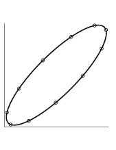
Figure 2. The constraint curve and the points of iterations for an 11-dimensional loop representation when $\alpha_{0}\approx 1.99$, $\alpha_{1}\approx 3.15$ and $c=1$.

7.3. Non-compact surfaces

The remaining surfaces will have one or two non-compact components (except for the surfaces in Section 7.4, which has both a compact and a non-compact component) and we will show that infinite representations always exist, whereas all finite dimensional representations are one-dimensional. By looking at the tables in Appendix B, one sees that non-compact surfaces appear only when $\alpha_{1}\leq 0$ which, for small $\hbar$, is equivalent to $\Delta\leq 0$. We can now prove the following result about the relation between geometry and representations.

Proposition 7.1.

Let $\mathcal{C}_{L,a}$ be an algebra corresponding to a surface $\Sigma$ where each component is non-compact, and assume that at least one of $\alpha_{0},\alpha_{1},c_{0}$ is different from zero. Then the following holds:

1. All finite dimensional irreducible representations have dimension one.

2. If $\Sigma$ has two components then there exists two inequivalent one-sided infinite dimensional irreducible representations, but no two-sided representations.

3. If $\Sigma$ is connected and non-singular, then there exists a two-sided infinite dimensional irreducible representation; if $a\leq 0$, or $a>0$ and $c>\mu^{2}(1+|\Delta|/4)$, then no one-sided representations exist. If $a>0$ and $c\leq\mu^{2}(1+|\Delta|/4)$ then one-sided representations exist.

Proof.

Statement 1 follows immediately from Proposition 5.8. Statement 2 can be proved in the following way: By examining all cases in Appendix B where $C^{-1}(0)$ has two non-compact components (Z.8, N.1, N.2, N.5, N.8), one sees that the components of $\Gamma$ which intersect $\mathbb{R}^{2}_{\geq 0}$ has the following form

In the first case, two inequivalent one-sided representations can be constructed but no two-sided representations can exist because backward or forward iterations of any point will eventually reach outside $\mathbb{R}^{2}_{>0}$. In the second case, it holds that the lower left tip of the curve intersecting $\mathbb{R}^{2}_{\geq 0}$ has strictly negative coordinates and the curve intersects the positive axes exactly once. This immediately allows for a construction of two inequivalent one-sided infinite dimensional representations. Now, can we have two-sided representations? Any constraint curve will cross the positive $r$-axis in the following points:

(7.3) $$r_{\pm}=\frac{1}{2}\Big{[}a\pm\sqrt{a^{2}+4\hat{c}_{1}}\Big{]}$$

If there is only one strictly positive intersection-point, it must hold that $r_{+}>0$ but $r_{-}\leq 0$. Actually $r_{-}<0$ since the lower left tip of the curve is not in $\mathbb{R}^{2}_{\geq 0}$. A necessary condition for a two-sided representations to exist is that there exists a point on the curve such that all backward and forward iterations by $\hat{L}$ is contained in $\mathbb{R}^{2}_{>0}$. This means that (since $\hat{L}$ preserves the direction of the curve) when we apply $\hat{L}$ to the point of intersection with the $s$-axis, we must obtain a point in $\mathbb{R}^{2}_{\geq 0}$ (otherwise no point is able to “jump” the negative part of $\Gamma$ by the action of $\hat{L}$). But this does not happen since

$$\hat{L}\begin{pmatrix}0\\ r_{+}\end{pmatrix}=\begin{pmatrix}-r_{+}+a\\ 0\end{pmatrix}=\begin{pmatrix}r_{-}\\ 0\end{pmatrix}\notin\mathbb{R}^{2}_{\geq 0}.$$

Let us now prove the statement 3. When $a\leq 0$ the are only two cases which give a connected non-singular non-compact surface, namely N.7 and N.10. In both cases, one can check that $\Gamma$ does not intersect the axes, and that at least one component is contained in $\mathbb{R}^{2}_{>0}$. Hence, no one-sided representations exist but two-sided representations exist.

When $a>0$ (Z.6, N.4) and $c>\mu^{2}(1+|\Delta|/4)$ then the component of $\Gamma$ that intersects $\mathbb{R}^{2}_{\geq 0}$ is contained in $\mathbb{R}^{2}_{>0}$, which implies that no one-sided representations exist, but two-sided representations exist. When $a>0$ and $c\leq\mu^{2}(1+|\Delta|/4)$ one component of the constraint curve will have the following form

In particular, it intersects the positive axes at least once. Thus, one-sided representations can be easily defined, but what about two-sided representations? We will now show that the backward and forward iteration of the point at the lower left tip both lie in $\mathbb{R}^{2}_{>0}$. We consider only the case Z.6 as the other case (N.4) can be treated analogously. The lower tip of the ellipse has coordinates $(r_{0},r_{0})$ for some $r_{0}>0$. We calculate

$$\hat{L}\begin{pmatrix}r_{0}\\ r_{0}\end{pmatrix}=\begin{pmatrix}r_{0}+a\\ r_{0}\end{pmatrix}\in\mathbb{R}^{2}_{>0}\quad\text{ and }\quad\hat{L}^{-1}\begin{pmatrix}r_{0}\\ r_{0}\end{pmatrix}=\begin{pmatrix}r_{0}\\ r_{0}+a\end{pmatrix}\in\mathbb{R}^{2}_{>0},$$

since $a>0$. Hence, we can define a two-sided representation by starting at $(r_{0},r_{0})$ and considering all backward and forward iterations by $\hat{L}$. ∎

The connected non-compact surfaces in Proposition 7.1 which allow for one-sided infinite dimensional representations correspond to surfaces with a narrow “throat” as in Figure 3.

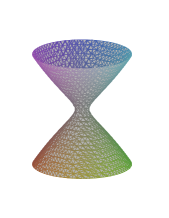
Figure 3. A connected non-compact surfaces which allows for one-sided representations.

This kind of “tunneling” is analogous to what happens for the compact surfaces. For a compact torus with a narrow hole, string representations can continue to exist; but as the hole grows wider they cease to exist. For non-compact surfaces, one-sided representations continue to exist even though the two components have been joined together. As an example, let us consider a surface with $\alpha_{0}=-1$, $\alpha_{1}=-1$ and $c=1.02$. Choosing $\hbar=0.3$, $\tilde{\delta}_{1}=\tilde{\beta}_{1}=-1/4$ and $\tilde{\gamma}_{1}=-1/2$ gives us the constraint curve in Figure 4. On the left curve, the first iterations of a one-sided infinite dimensional representations are plotted; on the right curve one finds iterations corresponding to a two-sided representation. The representations that are defined by these two figures the following form:

$$\phi_{\text{\small one-sided}}(W)\approx\begin{pmatrix}0&0.41&\\ &0&0.74\\ &&0&1.11\\ &&&0&1.53\\ &&&&\ddots&\ddots\end{pmatrix}$$

$$\phi_{\text{\small two-sided}}(W)\approx\begin{pmatrix}\ddots&\ddots&\\ &0&0.45\\ &&0&0.01\\ &&&0&0.01\\ &&&&0&0.45\\ &&&&&0&0.79\\ &&&&&&\ddots&\ddots\end{pmatrix}.$$

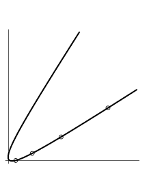
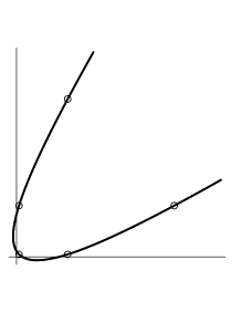
Figure 4. Constraint curves and iterations corresponding to a non-compact one-sheeted surfaces with $\alpha_{0}=-1$, $\alpha_{1}=-1$ and $c=1.02$.

Let us make a remark about the surface that has been excluded from Proposition 7.1, namely Z.2 with $c_{0}=0$. The polynomial reduces to $C(x,y,z)=z^{2}$ and the inverse image describes the $x,y$-plane. The constraint curve is the line $r-s=0$ and every point $(r,r)$ is a fix-point of $\hat{L}$. Hence, all irreducible representations are one-dimensional and the inequivalent representations are parametrized by the non-negative real numbers.

7.4. A surface with both compact and non-compact components

In the cases N.11 and N.12, the surface consists of two components: a non-compact surface and a compact surface of genus 0 (which collapses to a point when $\mu/\sqrt{c}=1$). The constraint curve will have the form as in Figure 5.

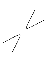
Figure 5. The constraint curve corresponding to a surface with both compact and non-compact components.

Thus, there is one component which allows for the construction of a finite dimensional string representation, and one component that induces a two-sided infinite dimensional representation. When $\mu/\sqrt{c}=1$, the lower component will intersect $\mathbb{R}^{2}_{\geq 0}$ in the point $(0,0)$, which allows for a one-dimensional trivial representation.

As for the compact surfaces, string representations do not exist for all values of $\hbar$ (if we fix $\hat{c}$). In the notation of Proposition 5.9, the condition for the existence of a $n$-dimensional string representation is

$$\mu\cosh\theta-\sqrt{\hat{c}}\cosh n\theta=0.$$

7.5. Singular non-compact surfaces

The surfaces Z.7, N.3, N.6 have a singularity at one point (which arises as two sheets come together) and the surface N.9 is a limit case of N.12, where the sphere touches the non-compact surface. The corresponding constraint curves will have one of the forms in Figure 6,

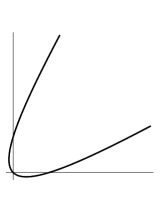
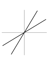
Figure 6. Constraint curves of singular non-compact surfaces.

where the left picture corresponds to Z.7 and N.3, and the right picture corresponds to N.6 and N.9. The left constraint curve clearly allows for two one-sided representations, but no two-sided representation can exist (cp. proof of Proposition 7.1). The right constraint curve allows for two different two-sided representations; it is easy to check that since $\hat{L}$ is invertible and $(0,0)$ is a fix-point, all iterations of a point on the curve in $\mathbb{R}^{2}_{>0}$ stay in $\mathbb{R}^{2}_{>0}$. That is, iterations approach the origin but never reach it. Furthermore, we note that no finite dimensional representations of dimension greater than one can exist.

7.6. Correspondence between geometry and representation theory

In [ABH⁺09], the representation theory of $\mathcal{C}_{L,a}$ was compared with the geometry of the inverse image for a class of compacts surfaces of genus 0 and 1. We have now extended this analysis to inverse images of general rotationally symmetric fourth order polynomials. Apart from recovering earlier results, we have shown that the representation theory respects the geometry of the surface to a high extent. Namely, in all cases where $\Sigma=C^{-1}(0)$ is empty, no representations exist. When $\Sigma$ is not a surface, then no irreducible representations of dimension greater than one exist. In the case when $\Sigma$ is non-singular non-compact, the correspondence is as follows: if $\Sigma$ has two sheets then there exists two inequivalent one-sided infinite dimensional representations, and if $\Sigma$ has one sheet there is a two-sided infinite dimensional representation. In all non-compact cases no finite-dimensional representations of dimension greater than one exist.

Appendix A – Solutions to system of equations

The general solution to the four equations

$$\begin{pmatrix}\alpha&\beta\\ \gamma&\delta\end{pmatrix}\begin{pmatrix}m&n\\ \tilde{m}&\tilde{n}\end{pmatrix}-\begin{pmatrix}m&n\\ \tilde{m}&\tilde{n}\end{pmatrix}\begin{pmatrix}\operatorname{tr}A&-\det A\\ 1&0\end{pmatrix}=0$$

is given by

$$n=\beta\tilde{m}-\delta m\qquad\tilde{n}=\gamma m-\alpha\tilde{m}.$$

If $\Delta=1+\det A-\operatorname{tr}A\neq 0$ then the system

(7.4) $$\bigg{[}\begin{pmatrix}\alpha&\beta\\ \gamma&\delta\end{pmatrix}-\mathds{1}_{2}\bigg{]}\begin{pmatrix}k\\ \tilde{k}\end{pmatrix}=\begin{pmatrix}m&n\\ \tilde{m}&\tilde{n}\end{pmatrix}\begin{pmatrix}a\\ 0\end{pmatrix}-\begin{pmatrix}u\\ v\end{pmatrix}$$

has a unique solution for $k$ and $\tilde{k}$. Whenever $a\neq 0$, we can always solve (7.4) by setting

$$m=\frac{1}{a}\Big{[}(\alpha-1)k+\beta\tilde{k}+u\Big{]}\qquad\tilde{m}=\frac{1}{a}\Big{[}\gamma k+(\delta-1)\tilde{k}+v\Big{]}.$$

If $\Delta=a=0$ there are two cases. When $A=\mathds{1}_{2}$ it is necessary that $u=v=0$, in which case (7.4) is identically satisfied and the affine map $L$ will be the identity map. If $A\neq\mathds{1}_{2}$ we get the following conditions

$$\alpha\neq 1:\qquad\text{if }(\alpha-1)v=\gamma u\text{ then }k=\frac{1}{1-\alpha}\big{(}u+\beta\tilde{k}\big{)}$$

$$\gamma\neq 0:\qquad\text{if }(\alpha-1)v=\gamma u\text{ then }k=-\frac{1}{\gamma}\big{(}v+(\delta-1)\tilde{k}\big{)}$$

$$\delta\neq 1:\qquad\text{if }(\delta-1)u=\beta v\text{ then }\tilde{k}=\frac{1}{1-\delta}\big{(}v+\gamma k\big{)}$$

$$\beta\neq 0:\qquad\text{if }(\delta-1)u=\beta v\text{ then }\tilde{k}=-\frac{1}{\beta}\big{(}u+(\alpha-1)k\big{)}.$$

Appendix B – Inverse images of $C(x,y,z)$

$\alpha_{1}>0$	$\alpha_{0}$	$c$	$\mu/\sqrt{c}$	$C^{-1}(0)$	$\Gamma\cap\mathbb{R}^{2}_{\geq 0}$
P.1	–	$<0$	–	$\emptyset$	$\emptyset$
P.2	$0$	$0$	–	$\{(0,0,0)\}$	$\{(0,0)\}$
P.3	$<0$	$0$	–	$\{(x,y,0):x^{2}+y^{2}=|\alpha_{0}|/\alpha_{1}\}$	$\left\{\frac{|\alpha_{0}|}{\alpha_{1}}(1,1)\right\}$
P.4	$>0$	$0$	–	$\emptyset$	$\emptyset$
P.5	$>0$	$>0$	$<-1$	$\emptyset$	$\emptyset$
P.6	$>0$	$>0$	$-1$	$\{(0,0,0)\}$	$\{(0,0)\}$
P.7	$\geq 0$	$>0$	$>-1$	Sphere	$\{\text{Ellipse}\}\cap\mathbb{R}^{+}_{0}$
P.8	$<0$	$>0$	$<1$	Sphere	$\{\text{Ellipse}\}\cap\mathbb{R}^{+}_{0}$
P.9	$<0$	$>0$	$1$	Surface with singularity	$\{\text{Ellipse}\}\cap\mathbb{R}^{+}_{0}$
P.10	$<0$	$>0$	$>1$	Torus	$\{\text{Ellipse}\}\cap\mathbb{R}^{+}_{0}$

$\alpha_{1}=0$	$\alpha_{0}$	$c_{0}$	$C^{-1}(0)$	$\Gamma\cap\mathbb{R}^{2}_{\geq 0}$
Z.1	$0$	$<0$	$\emptyset$	$\emptyset$
Z.2	$0$	$\geq 0$	$\{(x,y,\sqrt{c_{0}})\}\cup\{x,y,-\sqrt{c_{0}}\}$	Non-compact.
Z.3	$>0$	$<0$	$\emptyset$	$\emptyset$
Z.4	$>0$	$0$	$\{(0,0,0)\}$	$\{(0,0)\}$
Z.5	$>0$	$>0$	Sphere	Compact.
Z.6	$<0$	$<0$	One sheeted hyperboloid	Non-compact.
Z.7	$<0$	$0$	Singular hyperboloid	Non-compact.
Z.8	$<0$	$>0$	Two sheeted hyperboloid	Non-compact.

$\alpha_{1}<0$	$\alpha_{0}$	$c$	$\mu/\sqrt{c}$	$C^{-1}(0)$
N.1	$<0$	$\leq 0$	–	Two sheeted cone.
N.2	$<0$	$>0$	$<-1$	Two sheeted cone.
N.3	$<0$	$>0$	$-1$	One sheeted singular cone.
N.4	$<0$	$>0$	$>-1$	One sheeted cone.
N.5	$0$	$<0$	–	Two sheeted cone.
N.6	$0$	$0$	–	One sheeted singular cone.
N.7	$0$	$>0$	–	One sheeted cone.
N.8	$>0$	$<0$	–	Two sheeted cone.
N.9	$>0$	$0$	–	One sheeted cone $\cup$ sphere (singular).
N.10	$>0$	$>0$	$<1$	One sheeted cone.
N.11	$>0$	$>0$	$1$	One sheeted cone $\cup$ $\{(0,0,0)\}$.
N.12	$>0$	$>0$	$>1$	One sheeted cone $\cup$ sphere.

References

- [ABH+09] Joakim Arnlind, Martin Bordemann, Laurent Hofer, Jens Hoppe, and Hidehiko Shimada. Noncommutative Riemann surfaces by embeddings in . Comm. Math. Phys. (to appear), 2009. E-print: arXiv:0711.2588.
- [Arn08a] Joakim Arnlind. Graph Techniques for Matrix Equations and Eigenvalue Dynamics. PhD thesis, Royal Institute of Technology, 2008.
- [Arn08b] Joakim Arnlind. Representation theory of -algebras for a higher-order class of spheres and tori. J. Math. Phys., 49(5):053502, 13, 2008.
- [AS94] R. J. Archbold and J. S. Spielberg. Topologically free actions and ideals in discrete -dynamical systems. Proc. Edinburgh Math. Soc. (2), 37(1):119–124, 1994.
- [BHSS91] Martin Bordemann, Jens Hoppe, Peter Schaller, and Martin Schlichenmaier. and geometric quantization. Comm. Math. Phys., 138(2):209–244, 1991.
- [BR79] Ola Bratteli and Derek W. Robinson. Operator algebras and quantum statistical mechanics. Vol. 1. Springer-Verlag, New York, 1979. - and -algebras, algebras, symmetry groups, decomposition of states, Texts and Monographs in Physics.
- [BR81] Ola Bratteli and Derek W. Robinson. Operator algebras and quantum-statistical mechanics. II. Springer-Verlag, New York, 1981. Equilibrium states. Models in quantum-statistical mechanics, Texts and Monographs in Physics.
- [Dav96] Kenneth R. Davidson. -algebras by example, volume 6 of Fields Institute Monographs. American Mathematical Society, Providence, RI, 1996.
- [Eff65] Edward G. Effros. Transformation groups and -algebras. Ann. of Math. (2), 81:38–55, 1965.
- [Eff81] Edward G. Effros. Polish transformation groups and classification problems. In General topology and modern analysis (Proc. Conf., Univ. California, Riverside, Calif., 1980), pages 217–227. Academic Press, New York, 1981.
- [Eff82] Edward G. Effros. On the structure theory of -algebras: some old and new problems. In Operator algebras and applications, Part I (Kingston, Ont., 1980), volume 38 of Proc. Sympos. Pure Math., pages 19–34. Amer. Math. Soc., Providence, R.I., 1982.
- [Gli61a] James Glimm. Locally compact transformation groups. Trans. Amer. Math. Soc., 101:124–138, 1961.
- [Gli61b] James Glimm. Type I -algebras. Ann. of Math. (2), 73:572–612, 1961.
- [Jor88] Palle E. T. Jorgensen. Operators and representation theory, volume 147 of North-Holland Mathematics Studies. North-Holland Publishing Co., Amsterdam, 1988. Canonical models for algebras of operators arising in quantum mechanics, Notas de Matemática [Mathematical Notes], 120.
- [JSW95] P. E. T. Jorgensen, L. M. Schmitt, and R. F. Werner. Positive representations of general commutation relations allowing Wick ordering. J. Funct. Anal., 134(1):33–99, 1995.
- [Kar87] Gregory Karpilovsky. The algebraic structure of crossed products, volume 142 of North-Holland Mathematics Studies. North-Holland Publishing Co., Amsterdam, 1987. Notas de Matemática [Mathematical Notes], 118.
- [KTW85] Shinzō Kawamura, Jun Tomiyama, and Yasuo Watatani. Finite-dimensional irreducible representations of -algebras associated with topological dynamical systems. Math. Scand., 56(2):241–248, 1985.
- [Li92] Bing Ren Li. Introduction to operator algebras. World Scientific Publishing Co. Inc., River Edge, NJ, 1992.
- [Mac68] George W. Mackey. Induced representations of groups and quantum mechanics. W. A. Benjamin, Inc., New York-Amsterdam, 1968.
- [Mac76] George W. Mackey. The theory of unitary group representations. University of Chicago Press, Chicago, Ill., 1976. Based on notes by James M. G. Fell and David B. Lowdenslager of lectures given at the University of Chicago, Chicago, Ill., 1955, Chicago Lectures in Mathematics.
- [Mac89] George W. Mackey. Unitary group representations in physics, probability, and number theory. Advanced Book Classics. Addison-Wesley Publishing Company Advanced Book Program, Redwood City, CA, second edition, 1989.
- [NVO04] Constantin Năstăsescu and Freddy Van Oystaeyen. Methods of graded rings, volume 1836 of Lecture Notes in Mathematics. Springer-Verlag, Berlin, 2004.
- [NVO08] Erna Nauwelaerts and Freddy Van Oystaeyen. Introducing crystalline graded algebras. Algebr. Represent. Theory, 11(2):133–148, 2008.
- [OS89] V. L. Ostrovskiĭ and Yu. S. Samoĭlenko. Unbounded operators satisfying non-Lie commutation relations. Rep. Math. Phys., 28(1):91–104, 1989.
- [OS99] V. Ostrovskyi and Yu. Samoilenko. Introduction to the theory of representations of finitely presented *-algebras. I, volume 11 of Reviews in Mathematics and Mathematical Physics. Harwood Academic Publishers, Amsterdam, 1999. Representations by bounded operators.
- [ÖS08a] Johan Öinert and Sergei D. Silvestrov. Commutativity and ideals in algebraic crossed products. J. Gen. Lie Theory Appl., 2:287–302, 2008.
- [ÖS08b] Johan Öinert and Sergei D. Silvestrov. Commutativity and ideals in pre-crystalline graded rings. Preprints in Mathematical Sciences 2008:17, Centre for Mathematical Sciences, Lund University, 2008.
- [ÖS08c] Johan Öinert and Sergei D. Silvestrov. On a correspondence between ideals and commutativity in algebraic crossed products. J. Gen. Lie Theory Appl., 2(3):216–220, 2008.
- [ÖS09] Johan Öinert and Sergei D. Silvestrov. Crossed product-like and pre-crystalline graded rings. In V. Abramov, E. Paal, Sergei D. Silvestrov, and A. Stolin, editors, Generalized Lie theory in Mathematics, Physics and Beyond, chapter 24, pages 281–296. Springer-Verlag, Berlin, Heidelberg, 2009.
- [ÖSTAV08] Johan Öinert, Sergei D. Silvestrov, T. Theohari-Apostolidi, and H. Vavatsoulas. Commutativity and ideals in strongly graded rings. Preprints in Mathematical Sciences 2008:13, Centre for Mathematical Sciences, Lund University, 2008.
- [Pas89] Donald S. Passman. Infinite crossed products, volume 135 of Pure and Applied Mathematics. Academic Press Inc., Boston, MA, 1989.
- [Ped79] Gert K. Pedersen. -algebras and their automorphism groups, volume 14 of London Mathematical Society Monographs. Academic Press Inc. [Harcourt Brace Jovanovich Publishers], London, 1979.
- [Sak71] Shôichirô Sakai. -algebras and -algebras. Springer-Verlag, New York, 1971. Ergebnisse der Mathematik und ihrer Grenzgebiete, Band 60.
- [Sam91] Yu. S. Samoĭlenko. Spectral theory of families of selfadjoint operators, volume 57 of Mathematics and its Applications (Soviet Series). Kluwer Academic Publishers Group, Dordrecht, 1991. Translated from the Russian by E. V. Tisjachnij.
- [Sil95] Sergei D. Silvestrov. Representations of Commutation Relations. A Dynamical Systems Approach. PhD thesis, Departement of Mathematics, Umeå University, 1995. Published in Hadronic Journal Supplement vol. 11 116 pp, 1996.
- [SSdJ07a] Christian Svensson, Sergei Silvestrov, and Marcel de Jeu. Dynamical systems and commutants in crossed products. Internat. J. Math., 18(4):455–471, 2007.
- [SSdJ07b] Christian Svensson, Sergei D. Silvestrov, and Marcel de Jeu. Dynamical systems associated with crossed products. Preprint in Mathematical Sciences 2007:22, Centre for Mathematical Sciences, Lund University, 2007. E-print: arXiv:0807.2940. To appear in Acta Applicandae Mathematicae.
- [SSdJ09] Christian Svensson, Sergei D. Silvestrov, and Marcel de Jeu. Connections between dynamical systems and crossed products of Banach algebras by . In J. Janas, P. Kurasov, A. Laptev, S. Naboko, and G. Stolz, editors, Methods of Spectral Analysis in Mathematical Physics, volume 186 of Operator Theory: Advances and Applications, pages 391–401. Birkhäuser, Basel, 2009.
- [ST02] Sergei D. Silvestrov and Jun Tomiyama. Topological dynamical systems of type I. Expo. Math., 20(2):117–142, 2002.
- [ST08] Christian Svensson and Jun Tomiyama. On the commutant of in -crossed products by and their representations. Preprint in Mathematical Sciences 2008:21, Centre for Mathematical Sciences, Lund University, 2008. E-print: arXiv:0807.2940. To appear in J. Funct. Anal.
- [ST09] Christian Svensson and Jun Tomiyama. On the Banach -algebra crossed product associated with a topological dynamical system. Leiden Mathematical Institute report 2009:03, Leiden Mathematical Institute, 2009. E-print: arXiv:0902.0690.
- [SW96] Sergei D. Silvestrov and Hans Wallin. Representations of algebras associated with a Möbius transformation. J. Nonlinear Math. Phys., 3(1-2):202–213, 1996. Symmetry in nonlinear mathematical physics, Vol. 2 (Kiev, 1995).
- [Tak79] Masamichi Takesaki. Theory of operator algebras. I. Springer-Verlag, New York, 1979.
- [Tom87] Jun Tomiyama. Invitation to -algebras and topological dynamics, volume 3 of World Scientific Advanced Series in Dynamical Systems. World Scientific Publishing Co., Singapore, 1987.
- [Tom92] Jun Tomiyama. The interplay between topological dynamics and theory of -algebras, volume 2 of Lecture Notes Series. Seoul National University Research Institute of Mathematics Global Analysis Research Center, Seoul, 1992.
- [VS88] È. E. Vaĭsleb and Yu. S. Samoĭlenko. On the representation of the relations by an unbounded selfadjoint operator and a unitary operator. In Boundary value problems for differential equations (Russian), pages 30–52, ii. Akad. Nauk Ukrain. SSR Inst. Mat., Kiev, 1988.
- [VS90] È. E. Vaĭsleb and Yu. S. Samoĭlenko. Representations of operator relations by unbounded operators, and multidimensional dynamical systems. Ukrain. Mat. Zh., 42(8):1011–1019, 1990.