Primordial Trispectrum from Entropy Perturbations in Multifield DBI Model
Abstract:
We investigate the primordial trispectra of the general multifield DBI inflationary model. In contrast with the single field model, the entropic modes can source the curvature perturbations on the super horizon scales, so we calculate the contributions from the interaction of four entropic modes mediating one adiabatic mode to the trispectra, at the large transfer limit (). We obtained the general form of the 4-point correlation functions, plotted the shape diagrams in two specific momenta configurations, “equilateral configuration” and “specialized configuration”. Our figures showed that we can easily distinguish the two different momenta configurations.
1 Introduction
The Cosmic Microwave Background (CMB) provides us with remarkably detailed signatures of the early universe. The observations from large scale structures are consistent with an almost scale invariant, Gaussian primordial density perturbations generated during inflation. Precision measurements of any small deviation from Gaussian distribution enables us to distinguish different cosmological models. In the scalar field(s) inflation case, the non-Gaussian fluctuations can be parametrized by at the leading order and at sub-leading order respectively. The current experimental bound for the bispectrum (the three point correlation function of the primordial curvature perturbation ) is from WMAP5 [1], and for the trispectrum (four point correlation function) is [2], the next generation of experiments such as PLANCK will increase the sensitivity to about [3].
On the theoretical aspect, models with non-Gaussianities have been intensively investigated in recent years (see [4] for a review). Standard single-field slow-roll inflationary model predicts an almost Gaussian fluctuation with undetectable non-Gaussianity [5]. 3-point functions, or its Fourier transformation the bispectra for single-field and multifiled in slow-roll models are investigated in [6, 7, 48]. Higher-order correlation function, e.g. the trispectra (Fourier transformation of connected 4-point function) are studied in [8, 9, 10, 11, 12, 13]. For k-inflation models [17], DBI inflation models [18, 20, 19, 21] and curvaton scenario [14], the primordial bispectra and trispectra are calculated in [22, 23, 24, 25, 26, 27, 28, 29], in [30, 49] and in [15, 16] respectively. And the loop corrections to the power spectrum and bispectrum [32, 33, 46], the non-Gaussianities originated in noncommutative effect [34], vacuum [35], thermal fluctuations [38], string gas [37], matter bounce [36] are all investigated recently.
In this paper we will focus on the multiple fields DBI inflation model. For single field DBI models, the effective four-dimensional scalar field corresponds to the radial position of a brane in a higher dimensional warped conical geometry with other angular degree of freedom frozen for simplicity. However, if we consider the brane can also move in the angular directions, more than one effective scalars will turn on [47]. Generally the Lagrangian of the multifield DBI model can be expressed as with , where labels the multiple fields. And the trajectory of the background fields can be decomposed into one adiabatic mode which is along the direction of the trajectory and the other entropic modes which are orthogonal to the adiabatic direction. In contrast with the single field model, in which the curvature perturbations on uniform energy density hypersurfaces are conserved after horizon crossing, the curvature perturbations generally evolve in time even on large scales in the multifield models. The reason of this effect can be interpreted as due to the transfer between the adiabatic and entropic modes [39, 40, 41], so if there exists a large transfer from entropic modes to adiabatic mode, then the final curvature perturbations are mostly of entropic origin. Considering this effect, in this paper we calculate the contributions from the interaction of four entropic perturbations mediating one adiabatic perturbation to the trispectra in the general multifield scenario.
This paper is organized as follows. In Sec. II we firstly present the background setup, solve the equation of motion for the background fields, and secondly do the linear perturbations on the background, derive the second order action, and calculate the adiabatic and entropic power spectra in the massless limit. In first subsection of the Sec. III we calculate the 4-point correlation functions of the entropic perturbations from the interaction of four entropic modes mediating one adiabatic mode. In the second subsection we further analyze the shape function of the trispectra in two specific momenta configurations, one is the “equilateral configuration” another is the “specialized planar configuration”. In Sec IV. we conclude our results.
2 Review of generalized multifield model
In this section, we firstly review the setup of the general multifield model and the dynamics of the cosmological background, then concentrate on the linear perturbation theory, including the second order action and power spectra.
2.1 Setup and Background
In this subsection we briefly review the general multifield model which was proposed by Langlois et. al. in [23], where the Lagrangian is proposed to be of the form with , in particular, for the multifield DBI model the Lagrangian can be reduced into
| (1) |
where the determinant , is the warping factor and is the field space metric. As a specific example, such as the standard AdS throat, the warp factor depends only on one of the fields and takes form of (where depends on the flux numbers in specific string constructions).
Considering scalar fields coupled with gravity minimally, the action can be written as
| (2) |
with .
The energy-momentum tensor can be derived by varying with respect to the metric
| (3) |
where we define
| (4) |
In the last part of this section, we will investigate the background dynamics in the homogeneous and isotropic universe with the flat Friedmann-Robertson-Walker metric
| (5) |
where is the scale factor and is the Hubble parameter. Thus, from (3) we can see that the pressure is simply and the energy density can be expressed as
| (6) |
with and .
Following the assumption of metric (5), the equation of motion for scalar fields, the Friedmann equation and the continuity equation will be reduced to
| (7) | |||||
| (8) | |||||
| (9) |
2.2 Linear perturbation: Second order action and Power spectra
In this subsection, we will briefly mention the derivation of the second order action and derive the power spectra for the two fields DBI model. Following the standard approach which was proposed in [5], one can get the rigorous second order action of the general multifield inflation model
| (10) | |||||
where the explicit form of mass matrix and mixing matrix read
| (11) | |||||
| (12) |
In the derivation of (10), we used the ADM metric [44]
| (13) |
and chose the spatially flat gauge . In this gauge, the spatial part of the metric remains unperturbed, thus the physical degree of freedom are the perturbations of the multiple scalar fields which are denoted as . Generally the matrix (11) is not diagonal, so are not the canonical quantities which can be promoted to operators through canonical quantization procedure, so we must construct the canonical quantities in the next step. Fortunately, we can achieve our aim through decomposing into one adiabatic mode which is along the background trajectory in field space and entropic modes which are orthogonal to the trajectory, i.e.
| (14) |
where is the unit base vector which is along the trajectory, are the unit base vectors which are orthogonal to the trajectory, and they satisfy the normalized and orthogonal relation
| (15) |
In order to further simplify our calculation, we will assume the straight line background trajectory and flat field space metric, i.e., , and .
Before doing the orthogonal decomposition, we need to stop here and introduce the sound speed of perturbations in multifield DBI model. As illustrated in [23], the remarkable result of the action (1) is that all perturbations propagate at the same sound speed .
After introducing the sound speed in multifield DBI model, we can define a new field space metric as
| (16) | |||||
| (17) |
where represents the projection to the entropy direction and represents the projection to the adiabatic direction. Here we emphasize that the tilde metric is diagonal, and using this metric we can reduce (10) into
| (18) |
In order to gain some intuition, in what follows, we will restrict ourselves to a two field model , and it is straightforward to generalize our analysis to any number of fields. By virtue of (14), are decomposed into with and . After introducing three ”slow variation parameters” as in standard slow roll inflation
| (19) | |||||
| (20) | |||||
| (21) |
one can reduce (18) further
| (22) |
where we change the cosmic time into comoving time () and drop the last two sub-leading terms in (18) as in [23], because these two terms are suppressed by the slow roll parameters which are defined in (19). From (22), we can see that and are the canonical quantities, up to a normalization factor, which should be quantized, and the propagation speed of both the adiabatic mode and the entropy mode equal to .
Then we go to momentum space to do quantization, the Fourier mode of and can be quantized as
| (23) | |||||
| (24) |
where the creation and annihilation operators satisfy the standard communication relation , and we choose the Bunch-Davies vacuum
| (25) | |||||
| (26) |
It is now straightforward to calculate the two point functions
| (27) | |||||
| (28) | |||||
| (29) | |||||
| (30) |
where we set , and the Wightman functions for adiabatic and entropy modes read
| (31) | |||||
| (32) |
Then the power spectra of and are
| (33) | |||||
| (34) |
where the subscript indicates that the corresponding quantity is evaluated at the sound horizon crossing .
In single field model, the curvature perturbation () remains constant in the large scale limit due to the local energy conservation. However, in multifield model, the adiabatic perturbations can not produce the entropic perturbations, but the entropic perturbations can source the curvature perturbations on the large scales. Generally, the time dependence of the adiabatic and entropic perturbations on the superhorizon scales are always described by
| (35) |
with
| (36) |
and , are time dependent dimensionless functions. After performing the time integration for (35), one can get the general form of the transfer matrix which relate the curvature and entropic perturbations generated when a given mode crosses the sound horizon at time to those at some later time (on superhorizon scales)[23, 39, 45]
| (37) |
where
| (38) |
Substitute (36) into (37), one can obtain the relationship between the and with
| (39) |
where
| (40) |
and is the transfer coefficient which reflects the transfer between the adiabatic and entropic modes.
If , , i.e., the curvature perturbations on superhorizon scales are mainly transferred from the entropic perturbations. Thus the late time power spectrum of becomes
| (41) |
3 Trispectra from “scalar-exchanging” interaction
In this section, we will derive the general form of the 4-point correlation functions and plot the shape function (momentum dependence) for two special momenta configurations.
3.1 Four point correlation functions
In the first subsection, we will calculate the 4-point correlation functions for the entropic perturbations through the “scalar-exchanging” interaction. For this purpose, we firstly listed the third order action which has be derived in [23]
| (42) | |||||
As proved in [30], up to the third order, the Hamiltonian equals to the opposite Lagrangian , where the supper script “” denotes for the interaction picture
| (43) | |||||
| (44) | |||||
| (45) | |||||
| (46) | |||||
| (47) |
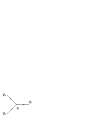
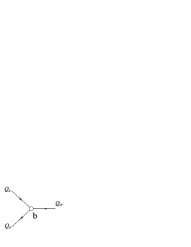
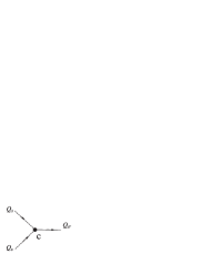
In what follows, we will still concentrate on the case. For this one, the main contributions to trispectra comes from the vertices with two external entropic legs , , and (see Fig. 1), because on the large scales the entropic perturbations source the curvature perturbations, i.e., we can approximately take .
Now, we are ready for calculating the 4-point correlation functions of the entropic perturbations . The “scalar-exchanging” interaction can be illustrated diagrammatically in Fig. 2, in which we merely plot one of the nine similar diagrams. Since there exist three different 3-point vertices, as shown in Fig. 1, the 4-point correlation functions of the entropic modes can be expressed as111The in-in formalism [43] which is often used in the literature in terms of a commutator form, is equivalent to the form (49) presented here.

| (48) |
with
| (49) | |||||
After some straightforward but lengthy calculations we can obtain the analytic expressions of the 4-point correlation functions of the entropic modes
| (50) | |||||
| (51) | |||||
| (52) | |||||
| (53) | |||||
| (54) | |||||
| (55) | |||||
| (56) | |||||
| (57) | |||||
| (58) | |||||
with
| (59) |
| (60) |
| (61) |
| (62) | |||||
| (63) | |||||
where denotes for the permutations between the momenta and .
Finally, we can get the general form of trispectra for the curvature perturbations , by virtue of (39) and (40)
| (64) | |||||
where in the second line we used the “slow variation parameters” defined in (19), and the function defined in the third line is called shape function, which we will analyze numerically in the next subsection.
3.2 Shapes of the trispectra
As we have obtained the general form of the trispectra, in this subsection, we will turn to plot the shape diagrams for the equilateral configuration with () and the “specialized planar” configuration with ().
Before the discussion of the shape functions, we note that the number of the independent arguments for the trispectra are six. In this paper, we choose six independent momenta , and one can also choose four independent momenta and two angles. In order for these momenta to form a tetrahedron (see Fig. 4), two conditions must be satisfied [31]:
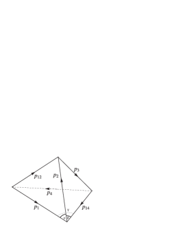
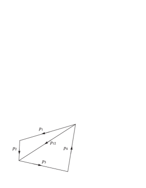
First, we define three angles at one vertex (see Fig. 4)
| (65) | |||||
| (66) | |||||
| (67) |
where these three angles should satisfy . This inequality is equivalent to
| (68) |
where we can take the equal sign when the tetrahedron reduces to a planar quadrangle.
Secondly, the six momenta should also satisfy all the triangle inequalities
| (69) |
and the last triangle inequality involving () is always satisfied given (68) and (3.2).
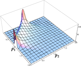
After discussing the two conditions which should be satisfied, now we will plot the shape function which is defined in (64). The first momenta configuration which we are interested in is called the “equilateral configuration” (). In this configuration, we plot the shape function versus and (see Fig. 6). And one can easily see from Fig. 6, that the amplitude of the shape function blows up on the circle with radius , which represents for the limit with ().
In the second case, we consider a specialized planar momenta configuration, i.e., the quadrangle with (see Fig. 4). As we have said, in the planar limit, (68) takes the equal sign, so we can obtain by solving (68)
| (70) |
where and are defined as
| (71) |
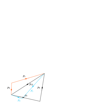
As pointed out in [31], the solution (blue) and solution (orange) in fact dual with each other (see Fig. 7), so we can choose arbitrary one to discuss, in the following we take the the solution.
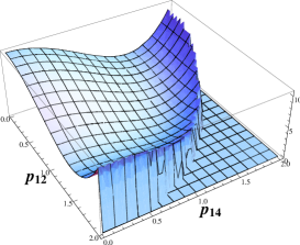
After setting and solving , the two independent arguments of the shape function are and , so, in this “specialized planar configuration”, we plot the shape function versus and (see Fig. 6). From Fig. 6, one can see that the shape function was highly-peaked at the “squeezed limit” ().
4 Conclusion
In this paper, we investigated the primordial trispectra produced by the “scalar-exchanging” interaction of the general multifield DBI inflationary model. In section 2, we studied the power spectra of the entropic modes and adiabatic modes without considering the mass term and the mixing term . In contrast with the single field model, the curvature perturbations generally evolve in time on the large scales in the multifield scenario, because the entropic modes can source the curvature perturbations on the super horizon scales, which can be described by the transfer coefficient . So, if the transfer process is strong (), the late time curvature perturbations will be mostly of the entropic origin.
Given that reason, in section 3, we calculate the contributions from the interaction of four entropic modes mediating one adiabatic mode to the trispectra. In subsection 3.1, we derived the general form of all the 4-point correlation functions, and in subsection 3.2, we further analyzed the shape function and plotted the shape diagrams for two specific momenta configuration “equilateral configuration” and “specialized planar configuration”. And our figures showed that one can easily distinguish the two types of configurations, because in the “equilateral configuration” the shape function blows up when was perpendicular to , or equivalent to say when , however, in the “specialized planar configuration” it was highly-peaked in the “squeezed limit” ().
Acknowledgments.
We thank Xingang Chen, Yi Wang, Eugene A. Lim for many useful discussions and comments, and KITPC-CAS for the conferences of connecting fundamental physics with observations. XG is grateful to Miao Li for reading the manuscript, BH is grateful to Rong-Gen Cai for the careful reading of the manuscript. BH is supported in part by the Chinese Academy of Sciences under Grant No. KJCX3-SYW-N2 and National Natural Science Foundation of China under Grant Nos. 10821504 and 10525060. XG was supported by the NSFC grant No.10535060/A050207, a NSFC group grant No.10821504 and Ministry of Science and Technology 973 program under grant No.2007CB815401.References
- [1] E. Komatsu et al. [WMAP Collaboration], “Five-Year Wilkinson Microwave Anisotropy Probe Observations:Cosmological Interpretation,” Astrophys. J. Suppl. 180, 330 (2009) [arXiv:0803.0547 [astro-ph]].
- [2] L. Alabidi and D. H. Lyth, “Inflation models and observation,” JCAP 0605, 016 (2006) [arXiv:astro-ph/0510441]. P. Creminelli, L. Senatore and M. Zaldarriaga, “Estimators for local non-Gaussianities,” JCAP 0703, 019 (2007) [arXiv:astro-ph/0606001].
- [3] N. Kogo and E. Komatsu, “Angular Trispectrum of CMB Temperature Anisotropy from Primordial Non-Gaussianity with the Full Radiation Transfer Function,” Phys. Rev. D 73, 083007 (2006) [arXiv:astro-ph/0602099]. T. Okamoto and W. Hu, “The Angular Trispectra of CMB Temperature and Polarization,” Phys. Rev. D 66, 063008 (2002) [arXiv:astro-ph/0206155].
- [4] N. Bartolo, E. Komatsu, S. Matarrese and A. Riotto, “Non-Gaussianity from inflation: Theory and observations,” Phys. Rept. 402, 103 (2004) [arXiv:astro-ph/0406398].
- [5] J. M. Maldacena, “Non-Gaussian features of primordial fluctuations in single field inflationary models,” JHEP 0305, 013 (2003) [arXiv:astro-ph/0210603].
- [6] D. Seery and J. E. Lidsey, “Primordial non-gaussianities in single field inflation,” JCAP 0506, 003 (2005) [arXiv:astro-ph/0503692].
- [7] D. Seery and J. E. Lidsey, “Primordial non-gaussianities from multiple-field inflation,” JCAP 0509, 011 (2005) [arXiv:astro-ph/0506056].
- [8] F. Arroja and K. Koyama, “Non-gaussianity from the trispectrum in general single field inflation,” Phys. Rev. D 77, 083517 (2008) [arXiv:0802.1167 [hep-th]].
- [9] D. Seery, J. E. Lidsey and M. S. Sloth, “The inflationary trispectrum,” JCAP 0701, 027 (2007) [arXiv:astro-ph/0610210]. D. Seery and J. E. Lidsey, “Non-gaussianity from the inflationary trispectrum,” JCAP 0701, 008 (2007) [arXiv:astro-ph/0611034].
- [10] D. Seery, M. S. Sloth and F. Vernizzi, “Inflationary trispectrum from graviton exchange,” arXiv:0811.3934 [astro-ph].
- [11] C. T. Byrnes, M. Sasaki and D. Wands, “The primordial trispectrum from inflation,” Phys. Rev. D 74, 123519 (2006) [arXiv:astro-ph/0611075].
- [12] K. T. Engel, K. S. M. Lee and M. B. Wise, “Trispectrum versus Bispectrum in Single-Field Inflation,” arXiv:0811.3964 [hep-ph].
- [13] Q. G. Huang, “The Trispectrum in the Multi-brid Inflation,” arXiv:0903.1542 [hep-th].
- [14] D. H. Lyth and D. Wands, “Generating the curvature perturbation without an inflaton,” Phys. Lett. B 524, 5 (2002) [arXiv:hep-ph/0110002].
- [15] N. Bartolo, S. Matarrese and A. Riotto, “On non-Gaussianity in the curvaton scenario,” Phys. Rev. D 69, 043503 (2004) [arXiv:hep-ph/0309033]. D. H. Lyth, “Non-gaussianity and cosmic uncertainty in curvaton-type models,” JCAP 0606, 015 (2006) [arXiv:astro-ph/0602285]. M. Sasaki, J. Valiviita and D. Wands, “Non-gaussianity of the primordial perturbation in the curvaton model,” Phys. Rev. D 74, 103003 (2006) [arXiv:astro-ph/0607627]. H. Assadullahi, J. Valiviita and D. Wands, “Primordial non-Gaussianity from two curvaton decays,” Phys. Rev. D 76, 103003 (2007) [arXiv:0708.0223 [hep-ph]].
- [16] Q. G. Huang, “Large Non-Gaussianity Implication for Curvaton Scenario,” Phys. Lett. B 669, 260 (2008) [arXiv:0801.0467 [hep-th]]. Q. G. Huang and Y. Wang, “Curvaton Dynamics and the Non-Linearity Parameters in Curvaton Model,” JCAP 0809, 025 (2008) [arXiv:0808.1168 [hep-th]]. P. Chingangbam and Q. G. Huang, “The Curvature Perturbation in the Axion-type Curvaton Model,” arXiv:0902.2619 [astro-ph.CO]. M. Li, C. Lin, T. Wang and Y. Wang, “Non-Gaussianity, Isocurvature Perturbation, Gravitational Waves and a No-Go Theorem for Isocurvaton,” arXiv:0805.1299 [astro-ph]. Q. G. Huang, “Spectral Index in Curvaton Scenario,” Phys. Rev. D 78, 043515 (2008) [arXiv:0807.0050 [hep-th]].
- [17] C. Armendariz-Picon, T. Damour and V. F. Mukhanov, “k-Inflation,” Phys. Lett. B 458, 209 (1999) [arXiv:hep-th/9904075]. J. Garriga and V. F. Mukhanov, “Perturbations in k-inflation,” Phys. Lett. B 458, 219 (1999) [arXiv:hep-th/9904176].
- [18] E. Silverstein and D. Tong, “Scalar Speed Limits and Cosmology: Acceleration from D-cceleration,” Phys. Rev. D 70, 103505 (2004) [arXiv:hep-th/0310221]. M. Alishahiha, E. Silverstein and D. Tong, “DBI in the sky,” Phys. Rev. D 70, 123505 (2004) [arXiv:hep-th/0404084].
- [19] G. Shiu and B. Underwood, “Observing the Geometry of Warped Compactification via Cosmic Inflation,” Phys. Rev. Lett. 98, 051301 (2007) [arXiv:hep-th/0610151]. S. Kecskemeti, J. Maiden, G. Shiu and B. Underwood, “DBI inflation in the tip region of a warped throat,” JHEP 0609, 076 (2006) [arXiv:hep-th/0605189].
- [20] X. Chen, “Multi-throat brane inflation,” Phys. Rev. D 71, 063506 (2005) [arXiv:hep-th/0408084]. X. Chen, “Inflation from warped space,” JHEP 0508, 045 (2005) [arXiv:hep-th/0501184].
- [21] S. E. Shandera and S. H. Tye, “Observing brane inflation,” JCAP 0605, 007 (2006) [arXiv:hep-th/0601099].
- [22] X. Chen, M. x. Huang, S. Kachru and G. Shiu, “Observational signatures and non-Gaussianities of general single field inflation,” JCAP 0701, 002 (2007) [arXiv:hep-th/0605045].
- [23] D. Langlois, S. Renaux-Petel, D. A. Steer and T. Tanaka, “Primordial perturbations and non-Gaussianities in DBI and general multi-field inflation,” Phys. Rev. D 78, 063523 (2008) [arXiv:0806.0336 [hep-th]].
- [24] D. Langlois, S. Renaux-Petel, D. A. Steer and T. Tanaka, “Primordial fluctuations and non-Gaussianities in multi-field DBI inflation,” Phys. Rev. Lett. 101, 061301 (2008) [arXiv:0804.3139 [hep-th]].
- [25] D. Langlois, S. Renaux-Petel and D. A. Steer, “Multi-field DBI inflation: introducing bulk forms and revisiting the gravitational wave constraints,” arXiv:0902.2941 [hep-th].
- [26] X. Gao, “Primordial Non-Gaussianities of General Multiple Field Inflation,” JCAP 0806, 029 (2008) [arXiv:0804.1055 [astro-ph]].
- [27] M. x. Huang, G. Shiu and B. Underwood, “Multifield DBI Inflation and Non-Gaussianities,” Phys. Rev. D 77, 023511 (2008) [arXiv:0709.3299 [hep-th]].
- [28] X. Chen, “Running non-Gaussianities in DBI inflation,” Phys. Rev. D 72, 123518 (2005) [arXiv:astro-ph/0507053].
- [29] F. Arroja, S. Mizuno and K. Koyama, “Non-gaussianity from the bispectrum in general multiple field inflation,” JCAP 0808, 015 (2008) [arXiv:0806.0619 [astro-ph]].
- [30] X. Chen, M. x. Huang and G. Shiu, “The inflationary trispectrum for models with large non-Gaussianities,” Phys. Rev. D 74, 121301 (2006) [arXiv:hep-th/0610235].
- [31] X. Chen, B. Hu, M. x. Huang, G. Shiu and Y. Wang, “Large Primordial Trispectra in General Single Field Inflation,” arXiv:0905.3494 [astro-ph.CO].
- [32] D. Seery, “One-loop corrections to a scalar field during inflation,” JCAP 0711, 025 (2007) [arXiv:0707.3377 [astro-ph]]. D. Seery, “One-loop corrections to the curvature perturbation from inflation,” JCAP 0802, 006 (2008) [arXiv:0707.3378 [astro-ph]].
- [33] E. Dimastrogiovanni and N. Bartolo, “One-loop graviton corrections to the curvature perturbation from inflation,” JCAP 0811, 016 (2008) [arXiv:0807.2790 [astro-ph]].
- [34] B. Chen, “Noncommutative inflation and non-Gaussianity,” Mod. Phys. Lett. A 23, 1577 (2008).
- [35] W. Xue and B. Chen, “-vacuum and inflationary bispectrum,” arXiv:0806.4109 [hep-th].
- [36] Y. F. Cai, W. Xue, R. Brandenberger and X. Zhang, “Non-Gaussianity in a Matter Bounce,” arXiv:0903.0631 [astro-ph.CO].
- [37] B. Chen, Y. Wang, W. Xue and R. Brandenberger, “String Gas Cosmology and Non-Gaussianities,” arXiv:0712.2477 [hep-th].
- [38] B. Chen, Y. Wang and W. Xue, “Inflationary NonGaussianity from Thermal Fluctuations,” JCAP 0805, 014 (2008) [arXiv:0712.2345 [hep-th]].
- [39] D. Langlois and S. Renaux-Petel, “Perturbations in generalized multi-field inflation,” JCAP 0804, 017 (2008) [arXiv:0801.1085 [hep-th]].
- [40] S. Renaux-Petel and G. Tasinato, “Nonlinear perturbations of cosmological scalar fields with non-standard kinetic terms,” JCAP 0901, 012 (2009) [arXiv:0810.2405 [hep-th]].
- [41] X. d. Ji and T. Wang, “Curvature and Entropy Perturbations in Generalized Gravity,” arXiv:0903.0379 [hep-th].
- [42] D. Seery, J. E. Lidsey and M. S. Sloth, “The inflationary trispectrum,” JCAP 0701, 027 (2007) [arXiv:astro-ph/0610210].
- [43] S. Weinberg, “Quantum contributions to cosmological correlations,” Phys. Rev. D 72, 043514 (2005) [arXiv:hep-th/0506236].
- [44] R. L. Arnowitt, S. Deser and C. W. Misner, “The dynamics of general relativity,” arXiv:gr-qc/0405109.
- [45] D. Wands, N. Bartolo, S. Matarrese and A. Riotto, “An observational test of two-field inflation,” Phys. Rev. D 66, 043520 (2002) [arXiv:astro-ph/0205253].
- [46] H. R. S. Cogollo, Y. Rodriguez and C. A. Valenzuela-Toledo, “On the Issue of the Series Convergence and Loop Corrections in the Generation of Observable Primordial Non-Gaussianity in Slow-Roll Inflation. Part I: the Bispectrum,” JCAP 0808, 029 (2008) [arXiv:0806.1546 [astro-ph]]. Y. Rodriguez and C. A. Valenzuela-Toledo, “On the Issue of the Series Convergence and Loop Corrections in the Generation of Observable Primordial Non-Gaussianity in Slow-Roll Inflation. Part II: the Trispectrum,” arXiv:0811.4092 [astro-ph].
- [47] D. A. Easson, R. Gregory, D. F. Mota, G. Tasinato and I. Zavala, “Spinflation,” JCAP 0802, 010 (2008) [arXiv:0709.2666 [hep-th]].
- [48] S. H. Tye, J. Xu and Y. Zhang, “Multi-field Inflation with a Random Potential,” arXiv:0812.1944 [hep-th].
- [49] J. Khoury and F. Piazza, “Rapidly-Varying Speed of Sound, Scale Invariance and Non-Gaussian Signatures,” arXiv:0811.3633 [hep-th].