Modular networks with hierarchical organization: The dynamical implications of complex structure

Abstract

Several networks occurring in real life have modular structures that are arranged in an hierarchical fashion. In this paper, we have proposed a model for such networks, using a stochastic generation method. Using this model we show that, the scaling relation between the clustering and degree of the nodes is not a necessary property of hierarchical modular networks, as had previously been suggested on the basis of a deterministically constructed model. We also look at dynamics on such networks, in particular, the stability of equilibria of network dynamics and of synchronized activity in the network. For both of these, we find that, increasing modularity or the number of hierarchical levels tends to increase the probability of instability. As both hierarchy and modularity are seen in natural systems, which necessarily have to be robust against environmental fluctuations, we conclude that additional constraints are necessary for the emergence of hierarchical structure, similar to the occurrence of modularity through multi-constraint optimization as shown by us previously.

I Introduction

Structural patterns in complex networks occurring in biological, social and technological contexts, have been a focus of study by physicists for a decade, since the groundbreaking discovery of small-world property Watts98 and scale-free degree distribution Barabasi99 for many networks. One of the common features seen in many networks is the occurrence of modules, namely, subnetworks whose members are highly inter-connected but have few links to nodes outside the module. Many networks have also been seen to have hierarchical organization, i.e., they are composed of successive interconnected layers or inter-nested communities. In the literature, often the terms hierarchy and modularity have been used almost inter-changeably, although, as shown in Fig. 1, they represent distinct properties of the network. However, it is interesting to note that these two properties have been found to coexist in many networks occurring in real life Ravasz02 ; Sole04 ; Holme03 ; Krause03 , including the Internet Satorras01 ; Eriksen03 and the network of cortical areas in the cat brain Zhou06 .

Most of the complex systems seen in real life also have associated dynamics Strogatz01 , and the structural properties of such networks have been sought to be linked with their dynamical behavior Boccalett06 ; Barahona02 . In this respect, one of the questions of obvious significance is whether there is a relation between the stability of the dynamics against small perturbations in the dynamical variables and the specific arrangement of the network’s connections. If the perturbation decays quickly, so that it is unable to spread to the rest of the network, the network is said to be stable. Such a property is necessary if networks are to survive the noisy environment that characterizes the real world. It has sometimes been argued that, networks with larger number of nodes, links and stronger inter-connections are more stable. Such assertions are partly based on empirical observations, e.g., in ecology, where it has been found that more diverse and strongly connected ecosystems are more robust than their smaller, weakly connected counterparts Elton58 . On the other hand, theoretical work on the stability of model networks have suggested the opposite conclusion. In particular, according to the May-Wigner theorem May73 for random networks, increasing the complexity (as measured by the number of nodes, density of connections and dispersion of interaction strengths) always leads to decreased stability. However, this result is based on the study of networks whose connection topology shows none of the structures that are seen in real life networks, in particular, modularity and hierarchy. Therefore, it is of interest to see whether introducing hierarchical organization and modular structures can result in refutation of the May-Wigner theorem. Early work on the stability of simple, structured model networks McMurtrie75 seemed to indicate that such structures indeed promote stability, and this was also seen under certain conditions for hierarchically organized networks Hogg89 . However, a later study of hierarchical, as well as, modular networks, concluded that these are less stable than corresponding random networks Hastings92 . We revisit this problem in the present paper, by proposing a network model that exhibits both modular structure and hierarchical organization. In addition to looking at the stability of equilibria of the network dynamics, we also consider the stability of synchronization over the network. Although these two stability phenomena are superficially similar, they involve looking at different properties of the network. The issue of network synchronization, in particular, has assumed importance in recent years, owing to its connection with, e.g., brain dynamics Zhou06 .

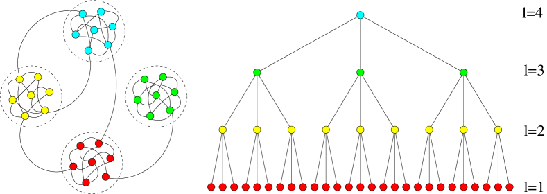
Figure 1: Schematic diagrams of (left) a modular network, with modules demarcated by broken circles, and (right) a hierarchical network with 4 levels, each indicated by a level number $l$.

An alternative model for hierarchical modular networks has been earlier proposed by Ravasz and Barabasi (RB) Ravasz03 . This model generates a set of inter-nested modules in a hierarchical fashion using a deterministic procedure that has both high clustering (because of the modular nature of the network at the most fundamental level) and a scale-free degree-distribution. These two properties do not always co-occur in other network models that have been proposed in the literature. In particular, the Barabasi-Albert (BA) network model Barabasi99 allows generation of a network with scale-free degree distribution through the preferential attachment mechanism, but the average clustering coefficient of its nodes decays with system size $N$. Further, in the RB model, a scaling relation is observed between the clustering coefficient of a node $C$ and its number of connections (i.e., degree) $k$:

$$C(k)\sim k^{-1}.$$ (1)

Similar relations were also observed in several real networks, such as the web of semantic connections between two English words which are synonyms Ravasz03 . This occurrence of the scaling relation between clustering and degree of the nodes in a network has often been taken as a signature for the existence of hierarchical modular structure in that network. Recently, this scaling relation was shown to be actually an outcome of degree-correlation bias in the usual definition of clustering coefficient Soffer05 .

However, it can be easily seen that this scaling relation is not a necessary indicator for the existence of either modularity or hierarchy. For example, consider a modular network consisting of $N$ nodes and $m$ modules of equal size. Let each node have degree $k$, with the links initially occurring exclusively between nodes belonging to the same module (i.e., the modules are isolated from each other). To make the network connected we rewire a small fraction of the links keeping the degree of each node fixed. Plotting clustering as a function of degree for this network will only show vertical spread of points at a single node degree value. Let us consider another example, this time a hierarchical structure, viz., the Cayley tree with $b$ branches at each vertex. Again, it is easy to see that the clustering versus degree curve will not show the characteristic scaling seen for the RB model. In fact, in the next section, we show that even for networks where both hierarchy and modularity are present, it is not necessary that this scaling relation between clustering and node degree will hold.

The paper is organized as follows. In the next section we introduced a simple model of a modular network with hierarchical organization. In section III we introduce the formalism to analyze the stability of dynamical equilibria and synchronized states of a network. The proposed model allows a detailed study of the relation between dynamical stability and hierarchical modular organization of the network. We observe that both of these structural properties actually increase the instability compared to an equivalent random network. This may appear counter-intuitive as both modularity and hierarchy are observed in networks occurring in nature, which necessarily have to be robust to survive environmental fluctuations. However, the emergence of modular structures can be understood as a response to multiple (and often conflicting) constraints imposed on such networks Pan07 . We conclude with a discussion about how these observations can possibly be extended to explain the emergence of hierarchical organization.

II Model of Hierarchical Modular Network

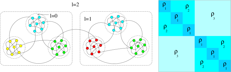
Figure 2: Schematic diagram of the hierarchical modular network model (left) with the modules occurring at the various hierarchical levels ($l$) indicated by broken lines, and the corresponding adjacency matrix (right) where $\rho_{1}$ indicates the density of connections within and, $\rho_{l+1}$, between the different modules at each level $l$.

Here we propose a general model for networks having modular as well as hierarchical structure. Let us begin with a modular network consisting of $m$ modules, each containing $n$ nodes. The connectivity (i.e., the probability of a link between any pair of nodes) within each module is $\rho_{1}$, while the connectivity between modules is $\rho_{2}$ ($\leq\rho_{1}$). We now introduce hierarchy by adding another set of $m$ modules (each having $n$ nodes) with the same $\rho_{1}$ and $\rho_{2}$. The nodes belonging to these two different sets of modules are now connected, but with a probability $\rho_{3}$ ($\leq\rho_{2}$). The resulting network has $2nm$ nodes and $l=2$ hierarchical levels (Fig. 2). To increase the number of hierarchical levels to $l=3$, we add a similar network with $2nm$ nodes to the existing network and, as above, add links between these two networks with a probability $\rho_{4}$ ($\leq\rho_{3}$). Thus, to get a network with $l=h$ hierarchical levels, the above procedure is repeated $h-1$ times. The final network contains $M=2^{h-1}m$ number of modules. Note that, all connections between nodes are made randomly. To reduce the number of model parameters, we assume that the connectivities $\rho_{1},\ldots,\rho_{h+1}$ are related as:

$$\frac{\rho_{2}}{\rho_{1}}=\frac{\rho_{3}}{\rho_{2}}=\cdots=\frac{\rho_{h+1}}{\rho_{h}}=r,$$ (2)

where, $0\leq r\leq 1$, the ratio of inter-modular connections between two successive hierarchical levels, is a control parameter. By varying $r$, one can switch between isolated modular ($r=0$) and homogeneous random ($r=1$) networks, with intermediate values of $r$ giving hierarchical modular networks. We compare between networks having different number of hierarchical levels $h$, keeping the total number of modules $M$ and average degree $\langle k\rangle$ fixed.

To consider the effect of hierarchy in isolation, while keeping modularity fixed (e.g., as measured by the Newman modularity measure $Q$ Newman04a ), we use a variant of the above model, where, $\rho_{1}$ = constant, while other connectivities are still related by

$$\frac{\rho_{3}}{\rho_{2}}=\cdots=\frac{\rho_{h+1}}{\rho_{h}}=r.$$ (3)

This implies that the average number of intra-modular ($\langle k_{\text{intra}}\rangle$) and inter-modular ($\langle k_{\text{inter}}\rangle$) connections per node are also constant .

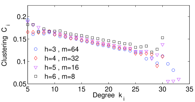
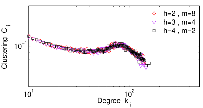
Figure 3: Clustering coefficient $C_{i}$ of the $i$-th node as a function of its degree $k_{i}$ for the hierarchical modular network model proposed here, where each module at $l=1$ is (left) a random ER network and (right) a scale-free BA network. The different symbols indicate networks with differing total number of hierarchical levels, $h$. For both types of networks, the total number of nodes is $N=8192$ with average intra-modular degree, $\langle k_{\text{intra}}\rangle=10$, inter-modular degree, $\langle k_{\text{inter}}\rangle=5$, and the ratio of inter-modular connections between two successive hierarchical levels, $r=0.1$. Note that, in neither case is a scaling relation observed between $C_{i}$ and $k_{i}$, although the modules are arranged in a hierarchical manner by construction.

The stochastic construction procedure of this network, along with the ability to vary modularity (by changing $r$) independently of the number of hierarchical levels ($h$), makes it an extremely general model. In addition, as it is hierarchical by construction, we can show that the criterion suggested in Ref. Ravasz03 , namely, the scaling relation between clustering and degree, is not a necessary condition for the existence of hierarchical modularity. As shown in Fig. 3 (left), when the modules are random networks, the scaling relation is clearly absent for our model network. To counter the possible argument that this failure of the relation is due to the non-scale-free degree distribution, we have also considered the case where each of the modules is a BA network. Although the inter-modular connections are made randomly, the network degree distribution is still scale-free. Even for this case, a clear scaling relation between clustering and degree is absent (Fig 3, right).

III Dynamics on Hierarchical Networks

III.1 Linear Stability of Equilibria

To look at the effect of hierarchy on network dynamics, we consider the linear stability of an arbitrarily chosen equilibrium state for a set of coupled differential equations defining the time-evolution of the system. For a network of $N$ nodes, a dynamical variable $x_{i}$ is associated with each node $i$. The state of the system, ${\bf x}$, can be characterized by $\dot{\bf x}=f({\bf x})$, where $f$ is a general nonlinear function. To investigate the stability around an arbitrary fixed point ${\bf{x}^{*}}$ (i.e., $f({\bf x})|_{\bf x^{*}}=0$), we check whether a small perturbation $\delta{\bf x}$ about ${\bf{x}^{*}}$ grows or decays with time. This perturbation evolves as

$$\dot{\delta{\bf x}}={\bf J}{\bf x},$$ (4)

where, ${\bf J}$ is the Jacobian matrix representing the interactions among the nodes: $J_{ij}=\partial f_{i}/\partial x_{j}|_{\bf{x}^{*}}$. As we are interested in the instability induced through the connections of the network, rather than the intrinsic instability of individual unconnected nodes, we can (without much loss of generality) set the diagonal element $J_{ii}=-1$. This implies that, in the absence of any connections, the nodes are self-regulating, i.e., the fixed point $\bf{x}^{*}$ is stable. The behavior of the perturbation is determined by the largest real part, $\lambda_{\text{max}}$, of the eigenvalues of ${\bf J}$. If $\lambda_{\text{max}}>0$, an initially small perturbation will grow exponentially with time, and the system will be rapidly dislodged from the equilibrium state ${\bf{x}^{*}}$.

The relation between the dynamical properties and the static structure of the network is provided by its adjacency matrix ${\bf A}$ (with $A_{ij}=1$, if nodes $i$ and $j$ are connected, and $0$ otherwise). There is a direct correspondence between the nature of the matrices ${\bf J}$ (specifying the dynamical behavior of perturbation) and ${\bf A}$ (which determines the structure of the underlying directed network), because $A_{ij}=0$ implies $J_{ij}=0$. In our model, we have generated $J_{ij}$ by randomly choosing the non-zero elements from a Gaussian distribution with zero mean and variance $\sigma^{2}$. For Erdos-Renyi (ER) random networks, ${\bf J}$ is an unstructured random matrix and the largest real part of its eigenvalues, $\lambda_{\text{max}}\sim\sqrt{N\rho\sigma^{2}}-1$, where $\rho$ is the connectivity of the network, and $\sigma$ measures the dispersion of interaction strengths May73 . When any of the parameters, $N$, $\rho$, or $\sigma$, is increased, there is a transition from stability to instability. The critical value at which the transition to instability occurs is $\sigma_{c}\sim 1/\sqrt{N\rho}$. This result, implying that complexity promotes instability, has been shown to be remarkably robust with respect to various generalizations Jirsa04 ; Sinha05 ; Sinha05a ; Sinha06 .

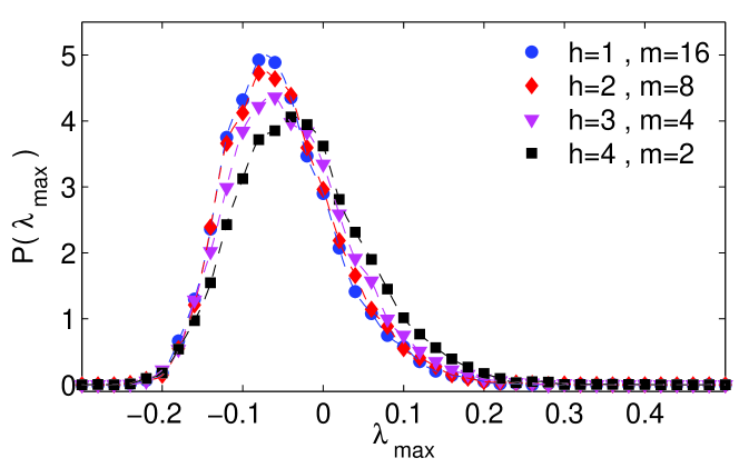
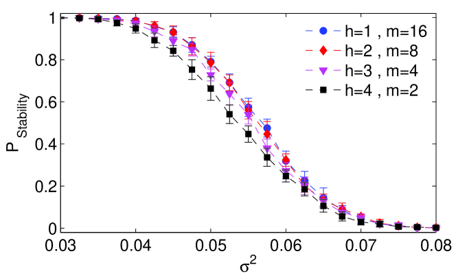
Figure 4: (Left) Probability distribution for the largest real part of the eigenvalues of the Jacobian $J$, as a function of total number of hierarchical levels, $h$ (the interaction strength parameter, $\sigma^{2}=0.05$). (Right) Probability of stability for a hierarchical modular network as a function of $\sigma^{2}$, with different symbols corresponding to differing total number of hierarchical levels $h$. Link weights are chosen from a $normal(0,\sigma^{2})$ distribution. For all cases, the network consists of $N=256$ nodes with average intra-modular degree, $\langle k_{\text{intra}}\rangle=10$, inter-modular degree, $\langle k_{\text{inter}}\rangle=5$, and the ratio of inter-modular connections between two successive hierarchical levels, $r=0.1$. At all hierarchical levels $l>1$, the network is split into two sub-networks. At $l=1$, each subnetwork is split into $m$ modules ($l=0$). Thus, $N=256$ nodes are divided equally among $2^{h-1}m=16$ modules, with the four curves corresponding to ($\Box$) $h=4$, $m=2$, ($\bigtriangledown$) $h=3$, $m=4$, ($\diamond$) $h=2$, $m=8$, and ($\circ$) $h=1$, $m=16$. Note that, increasing $h$ causes the transition to instability to occur at a smaller value of $\sigma^{2}$, implying that increasing hierarchy increases instability.

Here, using the above formalism, we examine the effect of hierarchy on the stability of equilibria when one of the network parameters (namely, $\sigma$) is varied. We study the critical value at which the transition to instability occurs, $\sigma_{c}$, as a function of the total number of hierarchical levels, $h$, keeping the total number of modules $M$ fixed. We find that, with increasing $h$, the distribution of $\lambda_{max}$ shifts towards more positive values (Fig. 4, left). As the system becomes unstable when $\lambda_{max}>0$, it follows that the probability of stability for the network decreases with increasing number of hierarchical levels (Fig. 4, right).

III.2 Synchronization

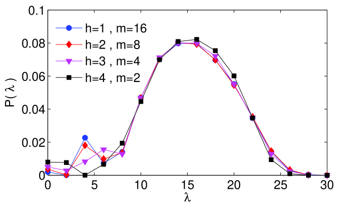
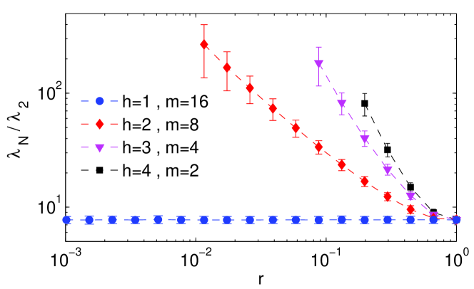
Figure 5: (Left) Probability distribution of eigenvalues of the Laplacian $L$, as a function of the total number of hierarchical levels, $h$ ($r=0.1$). (Right) The ratio of the largest eigenvalue ($\lambda_{N}$) to the second smallest eigenvalue ($\lambda_{2}$) as a function of $r$, the ratio of inter-modular connections between two successive hierarchical levels, with different symbols corresponding to differing total number of hierarchical levels $h$. For all cases, the network consists of $N=256$ nodes with average intra-modular degree, $\langle k_{\text{intra}}\rangle=10$ and inter-modular degree, $\langle k_{\text{inter}}\rangle=5$. At all hierarchical levels $l>1$, the network is split into two sub-networks. At $l=1$, each subnetwork is split into $m$ modules ($l=0$). Thus, $N=256$ nodes are divided equally among $2^{h-1}m=16$ modules, with the four curves corresponding to ($\Box$) $h=4$, $m=2$, ($\bigtriangledown$) $h=3$, $m=4$, ($\diamond$) $h=2$, $m=8$, and ($\circ$) $h=1$, $m=16$. Note that, increasing the number of hierarchical levels leads to divergence of the eigenratio, implying that synchronization becomes harder to achieve.

It is of interest to look not only at the stability of equilibria for network dynamics, but also at the stability of synchronized activity in networks. Let us consider a network of $N$ identical oscillators. The time-evolution of this coupled dynamical system is described by:

$$\dot{x}_{i}=\mathrm{F}(x_{i})+\epsilon\sum_{j=1}^{n}L_{ij}\mathrm{H}(x_{j}).$$ (5)

Here, $x_{i}$ is a variable associated with node $i$; $F$ and $H$ are evolution and output functions, respectively; $\epsilon$ is the strength of coupling; and ${\bf L}$ is the Laplacian matrix, defined as: $L_{ii}=k_{i}$, the degree of node $i$, $L_{ij}=-1$ if nodes $i$ and $j$ are connected, $0$ otherwise. It has been shown that the linear stability of the synchronized state $x_{s}$ (=$x_{1}=\ldots=x_{N}$) can be determined by diagonalizing the variational equation (Eq. 5) into $N$ blocks of the form, $\dot{y_{i}}=[DF(s)+\epsilon\lambda_{i}DH(s)]y_{i}$, where $y_{i}$ represent different modes of perturbation from the synchronized state. This is also referred to as the master stability equation Barahona02 . These equations have the same form but different effective couplings $\alpha_{i}=\epsilon\lambda_{i}$. The synchronized state is stable, i.e., the maximum Lyapunov exponent is in general negative, only within a bounded interval $[\alpha_{A},\alpha_{B}]$ Pecora98 . Let the eigenvalues of the Laplacian matrix be arranged as $0=\lambda_{1}<\lambda_{2}\leq\dots\leq\lambda_{n}$. Then, requiring all effective couplings to lie within the interval $\alpha_{A}<\epsilon\lambda_{2}\leq\dots\leq\epsilon\lambda_{N}<\alpha_{B}$, implies that a synchronized state is linearly stable, if and only if, $\lambda_{N}/\lambda_{2}<\alpha_{B}/\alpha_{A}$. Thus, a network having a smaller eigenratio $\lambda_{N}/\lambda_{2}$, is more likely to show stable synchronized activity.

Here, we obtain the eigenvalues of the Laplacian ${\bf L}$ for a hierarchical modular network (Fig. 5, left) and observe the eigenratio $\lambda_{N}/\lambda_{2}$ as a function of ratio of the inter-modular connections between two successive hierarchical levels, $r$, and the total number of hierarchical levels, $h$. First, keeping the number of hierarchical levels fixed, we vary the parameter $r$. We find that with decreasing $r$, i.e., as the number of connections between two successive hierarchical levels decrease, the instability of the synchronized state increases. Next, keeping the total number of modules fixed we increase the number of hierarchical levels ($h$) in the network. Fig. 5 (right) shows that as the number of hierarchal levels of the network is increased, $\lambda_{2}$ decreases, resulting in an increasing eigenratio. Thus, arranging the modules of a network in a hierarchical fashion also makes a network difficult to synchronize.

IV Discussion and Conclusion

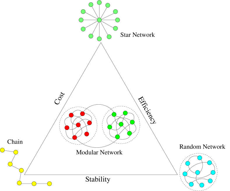
Figure 6: Schematic diagram indicating the different types of optimal networks obtained by satisfying different constraints. Each vertex represents networks obtained by satisfying a pair of constraints. Note that, modular networks emerge by optimizing all three constraints, viz., cost, efficiency and stability, indicated by the three arms of the triangle.

In previously published work Pan07 , we have shown that increased modularity in random networks leads to higher probability of instability for the equilibria of the network dynamics. Thus, the work presented here is an extension and generalization of the above result, demonstrating that increased number of hierarchical levels also tend to destabilize these equilibria, and moreover, the same phenomena is observed for the stability of synchronized activity in a network with respect to increased modularity and hierarchy. This raises the question of how can systems with hierarchical modular structures be seen in nature at all, where they have to be robust enough to survive constant environmental fluctuations. An answer to this can be fashioned along the lines of our recent work showing that additional natural constraints operating on networks in real life, such as the minimization of (a) resource cost for maintaining each link and (b) the time required for communicating between nodes, in addition to linear stability of equilibria, will make modular networks the optimal configuration (Fig. 6) Pan07 . We find such stable, modular networks to possess multiple hubs and a heterogeneous degree distribution. Many types of networks, including scale-free networks Barabasi99 , can be seen as special cases of this general criterion. Therefore, we can understand the large-scale occurrence of such networks in nature as a response to co-existing structural and dynamical constraints.

One can ask, what will be the effect of introducing constraints other than the ones mentioned here. For example, replacing the criterion for linear stability by one demanding robustness with respect to removal of links (selected by using a combination of random and targeted attack strategies) does not qualitatively change our results. It turns out that this criterion is satisfied by networks with bimodal degree distribution, a property that our optimal modular networks possess. However, while this can explain the ubiquity of modularity, it does not answer the question of why hierarchical organization is so common in nature. The fact that tree-like networks with extensive ramifications occur so often in the context of resource transport (e.g., the circulatory system in plants and animals) suggest that additional constraints related to flow maximization may be at work in this case. Another possible candidate for such a constraint may be the need to minimize wiring cost, i.e., the total link length Mathias01 . This is applicable when the network is embedded on a geographic (as opposed to topological) space, so that the wiring cost can been defined as the sum of the Euclidean distances between all connected pairs of nodes. As many of the networks showing hierarchical organization (such as the internet and the network of cortical areas in the brain) are indeed defined in metric space, this is a possibility that needs to be analysed in detail.

References

- (1) D. J. Watts and S. H. Strogatz. Nature 393, 440 (1998).
- (2) A.-L. Barabási and R. Albert. Science 286, 509 (1999).
- (3) E. Ravasz, A. L. Somera, D. A. Mongru, Z. N. Oltvai, and A.-L. Barabási. Science 297, 1551 (2002).
- (4) R. V. Solé and A. Munteanu. Europhys. Lett. 68, 170 (2004).
- (5) P. Holme, M. Huss, and H. Jeong. Bioinformatics 19, 532 (2003).
- (6) A. E. Krause, K. A. Frank, D. M. Mason, R. U. Ulanowicz, and W. W. Taylor. Nature 426, 282 (2003).
- (7) R. Pastor-Satorras and A. Vespignani. Phys. Rev. Lett. 86, 3200 (2001).
- (8) K. A. Eriksen, I. Simonsen, S. Maslov, and K. Sneppen. Phys. Rev. Lett. 90, 148701 (2003).
- (9) C. Zhou, L. Zemanová, G. Zamora, C. C. Hilgetag, and J. Kurths. Phys. Rev. Lett. 97, 238103 (2006).
- (10) S. H. Strogatz. Nature 410, 268 (2001).
- (11) S. Boccaletti, V. Latora, Y. Moreno, M. Chavez, and D.-U. Hwang. Physics Reports 424, 175 (2006).
- (12) M. Barahona and L. M. Pecora. Phys. Rev. Lett. 89, 054101 (2002).
- (13) C. S. Elton. The Ecology of Invasions by Animals and Plants. (Methuen, London, 1958).
- (14) R. M. May. Stability and Complexity in Model Ecosystems. (Princeton University Press, Princeton, NJ, 1973).
- (15) R. E. McMurtrie. J. Theor. Biology 50, 1 (1975).
- (16) T. Hogg, B. A. Huberman, and J. M. McGlade. Proc. Roy. Soc. Lond. B 237, 43 (1989).
- (17) H. M. Hastings, F. Juhasz, and M. A. Schreiber. Proc. Roy. Soc. Lond. B 249, 223 (1992).
- (18) E. Ravasz and A.-L. Barabási. Phys. Rev. E 67, 026112 (2003).
- (19) S. N. Soffer and A. Vázquez. Phys. Rev. E 71, 057101 (2005).
- (20) R. K. Pan and S. Sinha. Phys. Rev. E 76, 045103 (2007).
- (21) M. E. J. Newman and M. Girvan. Phys. Rev. E 69, 026113 (2004).
- (22) V. K. Jirsa and M. Ding. Phys. Rev. Lett. 93, 070602 (2004).
- (23) S. Sinha and S. Sinha. Phys. Rev. E 71, 020902(R) (2005).
- (24) S. Sinha. Physica A 346, 147 (2005).
- (25) S. Sinha and S. Sinha. Phys. Rev. E 74, 066117 (2006).
- (26) L. M. Pecora and T. L. Carroll. Phys. Rev. Lett. 80, 2109 (1998).
- (27) N. Mathias and V. Gopal. Phys. Rev. E 63, 021117 (2001).