Populating the Galaxy with Pulsars – II. Galactic dynamics

Abstract

Pulsar observations provide a suite of tests to which stellar and binary evolutionary theory may compare. Importantly, the number of pulsar systems found from recent surveys has increased the statistical significance of pulsar population synthesis results. To take advantage of this we are in the process of developing a complete pulsar population synthesis code that accounts for isolated and binary pulsar evolution, Galactic spatial evolution and pulsar survey selection effects. In a recent paper we described the first component of this code and explored how uncertainties in the parameters of binary and pulsar evolution affected the appearance of the pulsar population in terms of magnetic field and spin period. We now describe the second component which focusses on following the orbits of the pulsars within the Galactic potential. In combination with the first component we produce synthetic populations of pulsars within our Galaxy and calculate the resulting scale heights as well as the radial and space velocity distributions of the pulsars. Correlations between the binary and kinematic evolution of pulsars are also examined. Results are presented for isolated pulsars, binary pulsars and millisecond pulsars. We also test the robustness of the outcomes to variations in the assumed form of the Galactic potential, the birth distribution of binary positions, and the strength of the velocity kick given to neutron stars at birth. We find that isolated pulsars have a greater scale height than binary pulsars. This is also true when restricted to millisecond pulsars unless we allow for low-mass stars to be ablated by radiation from their pulsar companion in which case the isolated and binary scale heights are comparable. Double neutron stars are found to have a large variety of space velocities, in particular, some systems have speeds similar to the Sun. We look in detail at the predicted Galactic population of millisecond pulsars with black hole companions, including their formation pathways, and show where the short-period systems reside in the Galaxy. Some of our population predictions are compared in a limited way to observations but the full potential of this aspect will be realised in the near future when we complete our population synthesis code with the selection effects component.

1 Introduction

Detailed examinations of the stellar populations within the Galaxy, and indeed the greater Universe, have unearthed many fascinating objects. Examples of such systems are gamma-ray bursts (Klebesadel, Strong & Olson 1973; Paczynski 1986; Bogomazov, Lipunov & Tutukov 2008), coalescing double neutron stars (Rantsiou, Kobayashi, Laguna & Rasio 2008), X-ray binaries (Schreier et al. 1972; Liu, van Paradijs & van den Heuvel 2007; Galloway et al. 2008), microquasars (Margon et al. 1979; Abell & Margon 1979; Combi, Albacete-Colombo & Marti 2008) and millisecond pulsars (Backer et al. 1982; Manchester et al. 2005). Current belief suggests that all the aforementioned systems arise from binary stars in which both stars are close enough to experience a strong gravitational interaction with their companion. This may lead to mass transfer and depending upon the the mass ratio, types and ages of the two stars a plethora of different stellar and binary evolutionary phases may occur. Recent surveys spanning a large range of observed wavelengths now make it possible to monitor and analyse the combined properties of this variety of stellar populations. This in turn can place further constraints upon our theoretical understanding of stellar and binary evolution. For example, with the quickly increasing number of known low-mass stellar X-ray binary systems ($187$: Liu, van Paradijs & van den Heuvel 2007), high-mass X-ray binary systems ($114$; Liu, van Paradijs & van den Heuvel 2006) and pulsars ($>1600$; Manchester et al. 2005) it is possible to constrain features of neutron star (NS) and black hole (BH) formation from their relative Galactic scale heights. These have been examined for NS and BH low-mass X-ray binaries (via observations, Jonker & Nelemans 2004) showing evidence that (contrary to previous belief) BHs may receive momentum from their formation mechanism – the supernova (SN) event.

In this work our focus is on the Galactic population of pulsars. Observations of such objects occur primarily at radio (centimetre) wavelengths. These systems have intrinsically weak signals (typically measured in mJy: Lorimer 2005) and are observed as a regular series of pulses in time. Due to the frequency of the pulses we know these systems are compact (Hewish et al. 1968), while the period derivative allows evolutionary models of these systems to be developed (e.g. Goldreich & Julian 1969; Ostriker & Gunn 1969; Gunn & Ostriker 1970; Bisnovatyi-Kogan & Komberg 1974; van den Heuvel 1984; Kulkarni & Narayan 1988; Chen & Ruderman 1993) and tested (Dewey & Cordes 1987; Tauris & Bailes 1996; Dewi, Podsiadlowski & Pols 2005; Kiel, Hurley, Bailes & Murray 2008, hereafter Paper I). Finally, distances may be estimated from the dispersion of the pulse due to the electron density distribution within the Galaxy (Cordes & Lazio 2002). From these observations we now believe that pulsars are magnetic rotating neutron stars and that the radio signal arises from the magnetosphere and is well collimated. Timing of these radio pulses gives the spin period $P$ and the spin period derivative $\dot{P}$ from which the magnetic field and characteristic age of the pulsar may be inferred (see Paper I, and references therein for further details).

Knowledge of pulsar space velocities provides constraints on the effects of SNe on the NSs they give rise to. This may, in-turn, place constraints on the SN mechanism and NS structure. The birth velocities of pulsars (Lyne & Lorimer, 1994) combined with the work of Gott, Gunn & Ostriker (1970), Cordes, Romani & Ludgren (1993), Dewey & Cordes (1987) and Bailes (1989) demonstrated the necessity of asymmetric SN velocity kicks imparted on NSs by observing large isolated pulsar space velocities of order $1000$ km s^-1. Later studies also found similar conclusions, again because observations suggest pulsar space velocities in excess of the mean for normal field stars (Fryer & Kalogera, 2001). Evidence for asymmetric SNe is also provided by the misalignment of binary pulsar spin vectors to the orbital angular momentum vector (e.g. Kaspi et al. 1996). The vectors would normally be expected to be coupled before the violent SNe because of tidal effects and any occurrence of mass transfer (Bhattacharya & van den Huevel 1991; Hurley, Tout & Pols 2002). There is observational evidence of this misalignment for a number of pulsar binary systems including double NS systems (e.g. Kramer 1998).

Another method in which we are able to constrain the effects of SNe and to test the validity of our evolutionary assumptions (including the average magnitude of any kick delivered by a SN) is to compare, with observations, the kinematics of model pulsar populations within a model Galaxy (previous works include Dewey & Cordes 1987, Bailes 1989, Lorimer et al. 1993, Lyne et al. 1998 and Sun & Han 2004). There are two obvious pulsar populations we may recognise, those that are isolated pulsars and those pulsars within binary systems. We may make further distinction with regards to the spin of a pulsar – those of a ‘standard’ spin period ($P>1~{}$s), those of millisecond spin periods ($P<0.1~{}$s: known as millisecond pulsars, MSPs) while those between these two period ranges are known as partially spun-up or partially recycled pulsars. The final pulsar population which we wish to point out here are those pulsars which reside in double compact binaries, in particular double NS binaries (such as PSR $1913+16$: Hulse & Taylor 1975) and, within that population, double pulsar systems (PSR J$0737-3039$A&B: Burgay et al. 2003; Lyne et al. 2004).

From a simple evolutionary analysis of these systems (see Paper I) you may expect there to be distinct scale heights for each pulsar population within the Galaxy. This is assuming that all pulsars are given an asymmetric SN kick velocity drawn from the same distribution (i.e. ignoring the possible electron capture SN scenario which may confuse this issue: see Paper I; Podsaidlowski et al. 2004; Ivanova et al. 2008). Isolated pulsars – it is reasonable to presume – would have a greater scale height than those pulsars within binary systems. This is because binaries are on average heavier than single stars and also the binary orbit is able to absorb energy from the kick (as detailed in Hills 1983 and Tauris & Takens 1998). Having been previously ejected from a binary or having always been a single star would allow the kick velocity to have greater effect on the stellar space velocity. Isolated pulsars that have felt two SN kicks during their lifetime (one indirect and one direct) would be expected to have the largest scale height of any pulsar population (Bailes 1989). Say, for instance, that the first of two massive stars disrupts a binary system, giving momentum to both stars out of the Galactic plane, then the second massive star (now isolated) undergoes a SN and receives further momentum. Pulsars of different spin types, for example MSPs, can also be expected to have differing Galactic scale heights dependent upon the nature of their evolutionary histories. If one assumes a MSP forms via Roche-lobe overflow mass-transfer from a low mass companion the system only passes through one SN event and this will occur in a close binary which can overcome larger velocity kicks to stay bound than, say, a standard pulsar in a wider (pre-SN) orbit (e.g. Bailes 1989; Portegies Zwart & Yungleson 1998). If, however, some MSPs are formed via wind accretion from a high-mass companion (as discussed in Paper I), which may itself form a NS, a fraction of the MSP population may feel two kicks. This may lead to an increase of the MSP Galactic scale height and also produce a method for isolated MSP production (as described by Narayan, Piran & Shemi 1991 and Paper I). Finally, you may expect double pulsar systems to have a greater Galactic scale height than the single pulsar binary systems because they feel two SNe. However, the fact that the binary system had to survive these two kicks requires the kick velocity imparted from both events to be small enough (or well directed) for the binary to survive. Therefore, although two kicks occur it seems plausible that double pulsar systems may not attain a greater scale height than their isolated cousins (Pfahl, Podsiadlowski & Rappaport 2005; Dewi, Podsiadlowski & Pols 2005). Further to this simple analysis, the relative ages of each system type will also play an important role in the observable scale height, because older systems will have had more time to relax (outwards) in the Galactic gravitational potential – the distributions diffuse over time. For a more in-depth review of pulsar evolution and kinematics see the living review of Lorimer (2008).

The work described in this paper allows us to address these issues and to predict and compare the Galactic spatial distributions of pulsar populations. We follow on from our pulsar population synthesis in Paper I to not only evolve the stellar evolution of pulsars but move them within the Galactic gravitational potential. In other words we follow Galactic stellar, binary and kinematic evolution. As introduced in Paper I we are developing a code comprised of three modules: binpop (binary evolution), binkin (Galactic kinematics) and binsfx (synthetic survey simulations). An upcoming paper will describe the third module, binsfx, where we impose selection effects on the simulations, thus giving simulated data that can be compared directly to observations.

Section 2 outlines our binary evolution code (binpop) and details a necessary update to follow the evolution of a system that is disrupted owing to an asymmetric SN velocity kick. In Section 3 we describe the Galaxy kinematic code (binkin) which integrates the positions of pulsars – both in binary systems and isolated – forward in time within the Galaxy. This includes details of how the initial conditions for the Galactic population are chosen and the parameters involved. Results are given in Section 4 where, assuming a favoured binary and stellar evolutionary model of Paper I, we examine the pulsar population scale heights and velocities that arise from different binkin model assumptions. This includes a detailed examination of the MSP-BH binary population. In particular, we explore the formation and evolution of these systems. This is followed by a discussion of our findings and the main uncertainties involved in Section 5.

2 Rapid binary evolution

The first module, binpop, was described in detail in Paper I. Below we give an overview and also address the necessary modifications to binpop in order to correctly follow the Galactic positions of both members of a disrupted binary system.

2.1 BINPOP

binpop is a stellar/binary population synthesis package which convolves the binary stellar evolution (bse) code of Hurley, Tout & Pols (2002: hereafter HTP02) with realistic initial stellar and binary parameter distributions (as developed in Kiel & Hurley 2006 and Paper I). Stellar evolution is included according to the formulae presented in Hurley, Pols & Tout (2000). Meanwhile, bse attempts to account for all important binary evolutionary processes. These include tidal evolution, mass transfer, common envelope (CE) evolution, stellar mergers, magnetic braking, orbital gravitational radiation and supernovae velocity kicks. In Paper I extensive additions were made to bse, in terms of NS physics, so that pulsar evolution could be followed in detail. This means that aspects such as magnetic field decay, accretion induced field decay and spin-up, propeller evolution and pulsar death lines are now included. Inherent uncertainties in the variety of binary and pulsar evolutionary processes requires a host of parameterised prescriptions to be incorporated into bse. For example our lack of understanding of CE evolution is expressed as a parameter, $\alpha_{\rm CE}$, often referred to as the efficiency parameter. In terms of pulsar evolution there is the magnetic field decay time-scale, $\tau_{\rm B}$ and the accretion induced decay time-scale, $k$, for example, which are uncertain. Over time the uncertainty in many parameters has decreased – albeit slightly – due to a large array of simulations and increasingly detailed observations (e.g. Lyne et al. 1998; Portegies Zwart & Yungelson 1998; HTP02; Belczynski, Kalogera & Bulik 2002; Podsiadlowski, Rappaport & Han 2003; Sun & Han 2004; Yusifov & Kucuk 2004; Hobbs, Lorimer, Lyne & Kramer 2005; Kiel & Hurley 2006; Cordes et al. 2006; Lorimer et al. 2006; Ferrario & Wickramasinghe 2007; Liu, van Paradijs & van den Heuvel 2007; O’Shaughnessy, Kim, Kalogera & Belczynski 2008; Belczynski et al. 2008 and Paper I).

2.2 Binary evolution SN kick update

When following the kinematic evolution of a binary system within the Galaxy we require knowledge of the Galactic gravitational potential – the acceleration felt on the binary centre of mass (CofM) owing to the Galaxy – as well as any internal sources of momentum that arise. The primary stellar evolutionary phase that can perturb an orbit or disrupt a binary system is a SN. If the SN occurs in a binary and enough material is ejected from the system during the event (more than half of the total binary mass) the binary may disrupt (Hills 1983). Along with the assumed instantaneous mass loss, if there is any asymmetry in the explosion (which is arguable in the case of BHs, see Podsiadlowski, Rappaport & Han 2003 but note Pfahl, Podsiadlowski & Rappaport 2005), the newly formed compact star will receive a velocity kick which the binary CofM will feel (Shklovskii 1970; Lyne & Lormier 1994; Tauris & Takens 1998; HTP02). Depending upon the velocity kick direction and magnitude this may disrupt a binary or save it from mass loss-induced dissipation (Hills 1983; Kalogera 1998; Pfahl, Rappaport & Podsaidlowski 2003).

The algorithm described by HTP02 allows realistic orbital evolution modelling if the binary system survives the blast and stays gravitationally bound (eccentricity, $e<1$). However, because binary systems cease to exist once they become unbound, HTP02 were not troubled with calculating the recoil escape velocities of the two disassociated stars traveling on hyperbolic orbits with $e>1$. Now that the Galactic spatial kinematics of both binary systems and isolated stars is a concern, knowledge of all associated velocity changes are required. To this end we formulate a disruption model (in Section 2.2.1) and also describe similar methods derived by other groups (in Section 2.2.2). All methods considered here are generalised to allow for initially eccentric systems.

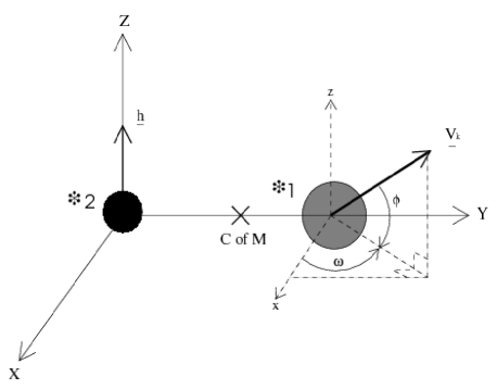
Figure 1: HTP02 orbital geometry as asymmetric SN occurs. Taken from Figure A1 of HTP02.

2.2.1 BSE disruption model

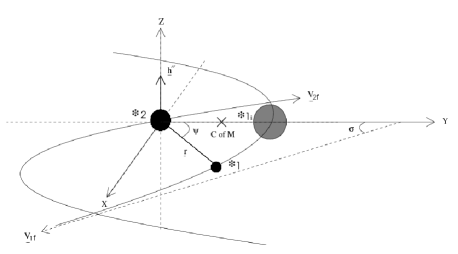
Figure 2: Orbital geometry of our disruption method after an asymmetric SNe.

Before one can calculate the final velocities of the disrupted stars the binary system must be known to disrupt. We start by considering what is already within the capabilities of the rapid binary evolution code (cf. Appendix A of HTP02) which we outline here. This assumes a reference frame in-which the pre-SN CofM is at rest, $\textbf{V}_{\rm s}=0$, and the secondary star (the star not exploding) is at the origin (as shown in Figure 1). The magnitude of the pre-SN relative orbital velocity is

$$V_{\rm orb}=\sqrt{\mu\left(\frac{2}{r}-\frac{1}{a}\right)}$$ (1)

and vectorily is

$$\textbf{V}=-V_{\rm orb}\left(\sin{\beta}\hat{\textbf{x}}+\cos{\beta}\hat{\textbf{y}}\right).$$ (2)

The separation of the two stars is $\textbf{r}=r[0,~{}1,~{}0]$ and $\beta$ is the angle between r and V. Also, $\mu=GM_{\rm b}$ where $G$ is the gravitational constant, $M_{\rm b}=M_{1}+M_{2}$ and the subscripts denote the particular star (the primary star being ₁ and the secondary ₂). In this reference frame the two pre-SN stellar velocities are,

$$\textbf{V}_{1}=\frac{M_{2}}{M_{\rm b}}\textbf{V}$$ (3)

and

$$\textbf{V}_{2}=-\frac{M_{1}}{M_{\rm b}}\textbf{V}.$$ (4)

Furthermore, the orbital angular momentum J is expressed as,

$$\textbf{J}=\frac{M_{1}M_{2}}{M_{\rm b}}\textbf{r}\times\textbf{V}=\frac{M_{1}M_{2}}{M_{\rm b}}\textbf{h}=M_{1}M_{2}\sqrt{\frac{l}{\mu}},$$ (5)

where h is the specific angular momentum (aligned with the z-axis) and $l=a\left(1-e^{2}\right)$ is the semi-latus rectum. The primary star, the SN progenitor, is about to explode and receive a momentum impulse arising from a velocity kick,

$$\textbf{V}_{\rm kick}=V_{\rm kick}\left(\cos{\omega}\cos{\phi}\hat{\textbf{x}}+\sin{\omega}\cos{\phi}\hat{\textbf{y}}+\sin{\phi}\hat{\textbf{z}}\right)$$ (6)

(where $\hat{\textbf{x}}$, $\hat{\textbf{y}}$ and $\hat{\textbf{z}}$ are the unit directions vectors). The kick speed, $V_{\rm kick}$, is modelled by a Maxwellian distribution,

$$P\left(V_{\rm kick}\right)=\sqrt{\frac{2}{\pi}}\frac{V_{\rm kick}^{2}}{V_{\sigma}^{3}}\exp^{-\frac{V_{\rm kick}^{2}}{2V_{\sigma}^{2}}},$$ (7)

as given by Hansen & Phinney (1997) with a dispersion $V_{\sigma}$. To facilitate any possible comparison to previous works, such as Hansen & Phinney (1997), Portegies Zwart & Yungelson (1998), HTP02 or Paper I, we take $V_{\sigma}=190~{}$km s^-1. However, a value of $265~{}$km s^-1 has more recently been suggested by Hobbs et al. (2005) and there have also been suggestions of a bimodal kick distribution (Arzoumanian, Chernoff & Cordes 2002). The direction of the kick is specified by chosing two angles $\omega$ and $\phi$ within the ranges $0<\omega<2\pi$ and $-\pi/2<\phi<\pi/2$ (as shown in Figure 1).

Immediately after the asymmetric SN event the new velocity of the proto-NS is

$$\textbf{V}^{{}^{\prime}}_{1}=\textbf{V}_{1}+\textbf{V}_{\rm kick}$$ (8)

and taking into account the instantaneous SN mass loss $\Delta M$ from the system we have a new relative velocity,

$$\textbf{V}^{{}^{\prime}}=\textbf{V}+\textbf{V}_{\rm kick}.$$ (9)

The velocity of the new centre of mass relative to the old centre of mass is

$$\textbf{V}^{{}^{\prime}}_{\rm s}=\frac{M_{\rm NS}}{M^{{}^{\prime}}_{\rm b}}\textbf{V}_{\rm kick}+\frac{\Delta MM_{2}}{M^{{}^{\prime}}_{\rm b}M_{\rm b}}\textbf{V}$$ (10)

(as in HTP02 equation A14). Following HTP02 the new eccentricity, $e^{{}^{\prime}}$, and semi-major axis, $a^{{}^{\prime}}$, of the system can then be calculated. If this gives an eccentricity greater than unity then the system is disrupted and we need expressions for the runaway velocities of the stars. For further details on the SN treatment and the evolution of binary systems which survive the event see HTP02.

Prior to the SN our chosen coordinate system had the orbital angular momentum vector directed along the $z$-axis but this will no longer be true for the post-SN system (unless $\textbf{V}_{\rm kick}=0$). However to simplify our post-SN calculations it is desirable to realign the vector with the $z$-axis. This realignment in the $x$-$z$ plane, owing to the SN, is performed by a rotation, $R_{\rm xz}$, around the y-axis such that the post-SN unaligned orbital specific angular momentum, $\textbf{h}^{{}^{\prime}}=\textbf{r}\times\textbf{V}^{{}^{\prime}}=[0,~{}r,~{}0]\times[V_{\rm x},~{}V_{\rm y},~{}V_{\rm z}]$ becomes $\textbf{h}^{{}^{\prime\prime}}=[0,~{}0,~{}h^{{}^{\prime\prime}}_{\rm z}]$. Note that we are using ${}^{{}^{\prime}}$ to denote the frame immediately after the SN and ${}^{{}^{\prime\prime}}$ when referring to the coordinate system of the frame after rotation. Here the rotation is guided by $\nu$, the angle between the pre- and post-SN angular momentum vectors (see Equation A13 of HTP02). This rotation matrix allows us to map our final velocities back onto the original coordinate system.

Now we consider the post-SN motion of the two stars which is governed by a hyperbolic conic section. We can no longer assume that the separation vector between the stars is aligned along the y-axis because the system is not necessarily at periastron. To account for this possible shift in coordinate system around the z-axis we calculate where in the orbit each star resides. Here we have

$$\cos{\psi}=\frac{1}{e^{{}^{\prime}}}\left(\frac{l^{{}^{\prime}}}{r}-1\right)=\frac{1}{e^{{}^{\prime}}}\left(\frac{(h^{{}^{\prime}})^{2}}{GM_{\rm b}^{{}^{\prime}}r}-1\right)$$ (11)

with $\psi$ defined to be positive in the positive y-direction and zero along the positive y-axis. There are two possible hyperbolic orbits for which each star may travel along – one in the positive y-region, the other in the negative y-region – which is governed by the direction of the y-component of the new relative velocity, that is, $\textbf{r}\cdot V^{{}^{\prime}}$. The sign of $\psi$ depends upon the the sign of the $\textbf{r}\cdot V^{{}^{\prime}}$ value, where $\psi<0$ when $\textbf{r}\cdot V^{{}^{\prime}}>0$. The post-SN binary mass must also be updated: $M^{{}^{\prime}}_{\rm b}=M_{\rm NS}+M_{2}$ with $M_{\rm NS}$ being the primary star mass. Using this and the new semi-major axis we may now calculate the final velocities of the two stars in the pre-SN centre of mass reference frame. Assuming a velocity at infinity, $\textbf{V}_{\infty}$, which is directed along an asymptote of the hyperbolic orbit we have final velocities for the two stars of

$$\textbf{V}_{\rm 1f}=\textbf{V}^{{}^{\prime}}_{\rm s}-R_{\rm xz}^{-1}\frac{\rm M_{2}}{M^{{}^{\prime}}_{\rm b}}\textbf{V}_{\infty}$$ (12)

and

$$\textbf{V}_{\rm 2f}=\textbf{V}^{{}^{\prime}}_{\rm s}+R_{\rm xz}^{-1}\frac{M_{\rm NS}}{M^{{}^{\prime}}_{\rm b}}\textbf{V}_{\infty}.$$ (13)

A simple calculation gives the magnitude,

$$V_{\infty}=\sqrt{\frac{GM^{{}^{\prime}}_{\rm b}}{a^{{}^{\prime}}}}.$$ (14)

The angle of the hyperbolic asymptote may be calculated from the angle $\sigma$ (as shown from Figure 2 which describes the post-SN coordinate system) where $\cos{\sigma}=1/e^{{}^{\prime}}$ (as in Tauris & Takens 1998) and $\sigma$ is always positive. This restricts $\sigma$ to range from $0\rightarrow\pi/2$. With our two angles we define the difference angle $\gamma=\sigma-\psi$ which is used in rotating the coordinate system around the z-axis. Separating $\textbf{V}_{\rm 1f}$ and $\textbf{V}_{\rm 2f}$ into component form gives us:

$$V_{\rm 1fx} = \frac{M_{\rm NS}}{M^{{}^{\prime}}_{\rm b}}V_{\rm kick}\cos{\omega}\cos{\phi}+\frac{\Delta MM_{2}}{M^{{}^{\prime}}_{\rm b}M_{\rm b}}V_{\rm orb}\sin{\beta}$$ (15)

$$-V_{\infty}\cos{\nu}\sin{\gamma},$$

$$V_{\rm 1fy} = \frac{M_{\rm NS}}{M^{{}^{\prime}}_{\rm b}}V_{\rm kick}\sin{\omega}\cos{\phi}+\frac{\Delta MM_{2}}{M^{{}^{\prime}}_{\rm b}M_{\rm b}}V_{\rm orb}\cos{\beta}$$ (16)

$$-V_{\infty}\cos{\gamma},$$

$$V_{\rm 1fz} = \frac{M_{\rm NS}}{M^{{}^{\prime}}_{\rm b}}V_{\rm kick}\sin{\phi},$$ (17)

$$V_{\rm 2fx} = \frac{M_{\rm NS}}{M^{{}^{\prime}}_{\rm b}}V_{\rm kick}\cos{\omega}\cos{\phi}+\frac{\Delta MM_{2}}{M^{{}^{\prime}}_{\rm b}M_{\rm b}}V_{\rm orb}\sin{\beta}$$ (18)

$$+V_{\infty}\cos{\nu}\sin{\gamma},$$

$$V_{\rm 2fy} = \frac{M_{\rm NS}}{M^{{}^{\prime}}_{\rm b}}V_{\rm kick}\sin{\omega}\cos{\phi}+\frac{\Delta MM_{2}}{M^{{}^{\prime}}_{\rm b}M_{\rm b}}V_{\rm orb}\cos{\beta}$$ (19)

$$+V_{\infty}\cos{\gamma}$$

and

$$V_{\rm 2fz} = \frac{M_{\rm NS}}{M^{{}^{\prime}}_{\rm b}}V_{\rm kick}\sin{\phi}.$$ (20)

We also account for coalescence of the two stars if the newly formed compact star velocity kick is directed towards the companion. Coalescence occurs if the companion radius, $R_{2}$, is greater than periastron or the distance of closest approach: if $R_{2}>a^{{}^{\prime}}(e^{{}^{\prime}}-1)$ we assume the stars coalesce (see also Tauris & Takens 1998; Belczynski et al. 2008) and the merger outcome has the final centre of mass velocity, $\textbf{V}^{{}^{\prime}}_{\rm s}$ and the mass of the NS and companion are combined (see HTP02 for further details of merger outcomes).

Equations 15 to 20 are the velocities calculated within the bse kick routine and are communicated into binkin. Before adding these to the Galactic binary centre of mass velocity at the time of SN it is first necessary to perform a random orientation of the pre-SN binary orbital plane, which until now has been fixed in the Galactic xy-plane. We randomly choose three Euler angles $\alpha_{\rm E}$, $\beta_{\rm E}$ and $\gamma_{\rm E}$, within the ranges $0\leq\alpha_{\rm E}{\rm,\gamma_{\rm E}<2\pi}$ and $0\leq\beta_{\rm E}<\pi$, to give a 3D rotation of the velocities in Equations 12 and 13. The post-SN velocities (pre-SN CofM velocity plus the rotated disruption velocities) are then used within the kinematic routine to calculate the subsequent velocities and positions within the Galaxy of the pulsar and its former companion.

2.2.2 Related disruption models

There are two other groups who have independently developed models for deriving the run-away velocities of stars from a disrupted binary. The method published recently by Belczynski et al. (2008) is similar to our demonstration and is also generalised for arbitrary eccentricity. The main difference is that it allows a velocity $\textbf{v}_{\rm imp}$ to be imparted to the secondary from the expanding shell of the SN. In our work we essentially assume that $\textbf{v}_{\rm imp}=0$ which has minimal effect except in some cases of small pre-SN orbital separation (Kalogera 1996; Belczysnki et al. 2008). Tauris & Takens (1998; hereafter T&T98) have developed a relatively sophisticated model. The major difference between our model and the T&T98 model is the coordinate system scheme and the latters assumption that the companion star may have momentum imparted directly onto it from the SN blast wave (as in Belczynski et al 2008 and Dewey & Cordes 1987). The companion star may also have some fraction of mass stripped off it and/or ablated owing to the impact of the shell of material ejected from the primary. To include the possibility of investigating the effect of these additional considerations we have worked through the T&T98 demonstration and implemented it as an option in bse, generalised to eccentric orbits. However, we do not exercise this option in this work.

2.2.3 Disruption model illustration

To illustrate the effect the binary orbit has on the runaway velocities of disrupted stars we produce a simple population of binary systems. For this population the primary mass, $M_{1}$, is randomly selected from a flat distribution ranging from $10-20~{}M_{\odot}$, the secondary mass, $M_{2}$, from a flat distribution ranging from $0.1-20~{}M_{\odot}$ and the orbital separation is selected randomly from a flat distribution from $1$ to $10~{}000~{}R_{\odot}$. All systems are initially circular to simplify the analysis. The radius of the secondary star is linked to its mass by $R_{2}=1.3M_{2}^{0.6}$ if $M_{2}$ is greater than unity and by $R_{2}=M_{2}$ otherwise. We make sure the system is not in contact at birth. We then let the primary undergo a SN that leaves a NS with $M_{NS}=1.4~{}M_{\odot}$ and assume the remnant is given a kick from Equation 7 with $V_{\sigma}=190~{}$km s^-1 (in accordance with Hansen & Phinney 1997). The post-SN velocities for disrupted stars are calculated using the bse method detailed above.

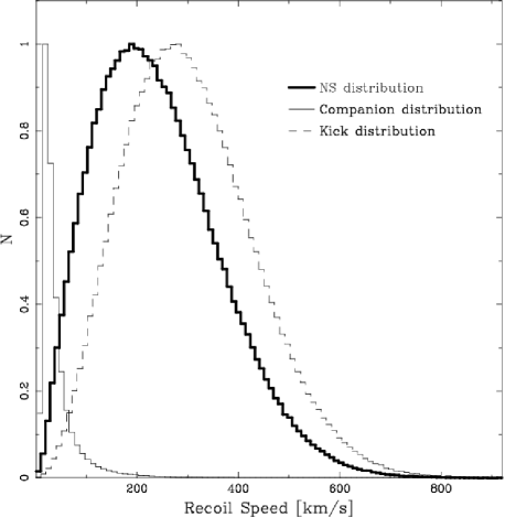
Figure 3: The speeds of the two stars following the SNe. The thick line represents the NS recoil speed distribution while the thin line is the companion recoil speed distribution. Included is the assumed asymmetric SN kick distribution assuming a dispersion of $190~{}$km s^-1 (dashed line).

After generating a million systems we find that the majority ($99\%$) become unbound and the incidence of coalescence is negligible. In Figure 3 we see the distributions of NS and companion star recoil speed and compare this to the $\textbf{V}_{\rm kick}$ distribution, i.e. the distribution for a population of standard single NSs. The first item we wish to note is the difference in the typical velocities received by both stars: the NS, which directly experiences the additional momentum imparted from the asymmetric SN, will most likely depart the binary system with a greater velocity than the companion star (relative to the CofM). The second point of interest is the similarity between the NS recoil speed distribution and the kick distribution. Clearly not all of the momentum imparted onto the NS goes into the NS recoil velocity, some of the momentum is instead transported into the CofM momentum, consumed by the disruption of the binary system and converted into additional velocity of the companion star. Therefore, although the shape of the NS recoil speed distribution is consistent with the kick distribution the NS distribution is shifted somewhat to lower values. In regards to this, observational pulsar velocity studies that do not account for the possibility of a fraction of the sample being disrupted from binary systems may underestimate the underlying SN kick distribution. It also suggests a possible mechanism for any bimodality found in the velocity structure of pulsar observations – similar to that found by Arzoumanian, Chernoff & Cordes (2002) from which they concluded a bimodal asymmetric SN kick distribution, or possibly binary disruption effects, could cause such detected velocities. We note that the form of the underlying orbital period (or separation) distribution of the model binaries will affect the distribution of recoil speeds – with an increased proportion of short-period systems leading to an increased difference between the NS recoil speed and kick distributions – and we have not explored this aspect in detail here.

3 Galactic kinematics

3.1 Galactic gravitational potentials

Much work over the years has lead to estimates of the Galactic gravitational potential. Miyamoto & Nagai (1975) generalised the work of Toomre (1963) who calculated flattened Plummer (1911) models for the Galaxy. Since then further observations have lead to estimates by Carlberg & Innanen (1987) of disk-halo, bulge and nucleus potentials which in turn have been updated by Kuijken & Gilmore (1989). Kuijken & Gilmore (1989) used more extensive observations of Galactic stellar densities, which allows the mapping to an assumed (to first order) smooth time-independent galactic gravitational potential.

The KG89 model potential is,

$$\Phi_{\textnormal{{\tiny G}}}^{KG} = \Phi_{\textnormal{{\tiny disk/halo}}}^{KG}+\Phi_{\textnormal{{\tiny nuc}}}^{KG}+\Phi_{\textnormal{{\tiny bulge}}}^{KG}$$ (21)

where,

$$\Phi_{\textnormal{{\tiny disk/halo}}}^{KG} = -\frac{GM_{\textnormal{{\tiny disk}}}}{\sqrt{\left(a+\sum_{\rm i=1}^{3}\beta_{i}\sqrt{z^{2}+h_{\rm i}^{2}}\right)^{2}+b^{2}+r^{2}}}$$ (23)

$$\Phi_{\textnormal{{\tiny nuc}}}^{KG} = -\frac{GM_{\textnormal{{\tiny nuc}}}}{\sqrt{b^{2}+r^{2}}}$$ (24)

$$\Phi_{\textnormal{{\tiny bulge}}}^{KG} = -\frac{GM_{\textnormal{{\tiny bulge}}}}{\sqrt{b^{2}+r^{2}}},$$ (25)

and the parameter values for each region are:

disk/halo:

$\beta_{1}=0.4$, $\beta_{2}=0.5$, $\beta_{3}=0.1$, $h_{1}=0.325~{}{\rm kpc}$, $h_{2}=0.090~{}{\rm kpc}$, $h_{3}=0.125~{}{\rm kpc}$, $a=2.4~{}{\rm kpc}$, $b=5.5~{}{\rm kpc}$, $M_{\rm disk}=1.45\times 10^{11}~{}M_{\odot}$

nucleus:

$b=0.25~{}{\rm kpc}$, $M_{\rm nuc}=9.3\times 10^{9}~{}M_{\odot}$

bulge:

$b=1.5~{}{\rm kpc}$, $M_{\rm bulge}=1.0\times 10^{10}~{}M_{\odot}$.

If necessary, use of the KG89 model allows us to compare results to previous binary pulsar population synthesis works such as Lorimer et al. (1993). While now considered somewhat outdated, the KG89 potential is still in use within recent observational works, such as, Freire, Ransom & Gupta (2007) who use it in their calculation of the pulsar spin period when accounting for observational effects of the acceleration between the Solar System Barycentre and NGC 1851 - the globular cluster in which their observed pulsar resides. However, a recent appraisal of the most promising Galactic gravitational potentials to use was completed by Sun & Han (2004). Their favoured method for ease of implementation is that given by Paczynski (1990: see below). Sun & Han (2004) also commented favourably on the work of Dehnen & Binney (1998) who fit a multi-parameter mass model to kinematic data of the Milky Way. Sun & Han (2004) found that the Dehnen & Binney (1998) model is overly complicated to set up and manipulate, while the simpler Paczynski (1990, hereafter P90) model is as accurate as the Dehnen & Binney (1998) model. As such we also include the P90 model in our work.

The P90 model, like the KG89 model, follows the potential of Miyamoto & Nagai (1975) for the disk ($i=1$) and spheroid components ($i=2$). Equation 9 of Paczynski (1990) is,

$$\Phi_{i}^{\rm P}(R,z)=-\frac{GM_{i}}{\left(R^{2}+\left[a_{i}+(z^{2}+b_{i}^{2})^{(1/2)}\right]^{2}\right)^{(1/2)}},$$ (26)

where $R=\sqrt{(}x^{2}+y^{2})$. The P90 model, however, differs from the KG89 model not only with the assumed constant values used within Equation 26 (for the disk potential) but also with the assumed form of the halo potential,

$$\Phi_{\rm h}^{\rm P}(r)=-\frac{GM_{\rm h}}{r_{\rm h}}\left[\frac{1}{2}\ln(1+\frac{r^{2}}{r_{\rm h}^{2}})+\frac{r_{\rm h}}{r}~{}{\rm atan}\left(\frac{r}{r_{\rm h}}\right)\right],$$ (27)

where $r^{2}=R^{2}+z^{2}$ is used to simplify the equation. The parameters being:

disk (i = 1):

$a_{1}=0~{}{\rm kpc},~{}b_{1}=0.277~{}{\rm kpc},~{}M_{1}=1.12\times 10^{10}~{}M_{\odot}$,

spheroid (i = 2):

$a_{2}=3.7~{}{\rm kpc},~{}b_{2}=0.20~{}{\rm kpc},~{}M_{2}=8.07\times 10^{10}~{}M_{\odot}$,

halo (i = h):

$r_{\rm h}=6.0~{}{\rm kpc},~{}M_{\rm h}=5.0\times 10^{10}~{}M_{\odot}$.

The KG89 and P90 models are both based on old observations of the stellar neighbourhood. As such, these models are only considered accurate out to a radii of $\sim 12$ kpc. More recent observations completed in the Sloan Digital Sky Survey (SDSS: York et al. 2000), within the Sloan Extension for Galactic Understanding and Exploration (SEGUE: Lee et al. 2008) program, have allowed the Galactic gravitational potential to be measured out to a radii of $\sim 60$ kpc (Xue et al. 2008). To do this Xue et al. (2008) have made line of sight velocity measurements of $\sim 2500$ blue horizontal branch stars which are converted into circular velocity estimates of the Milky Way. Ultimately the work of Xue et al. (2008) is completed to probe the halo of our Galaxy and thus they do not examine in any detail the inner Galactic potential. However, at this stage we consider their complete assumed Galactic gravitational potential as an option in our work. The Xue et al. (2008, hereafter Xue08) model makes use of the following exponential disk, Hernquist (1990) bulge and Navarro, Frenk & White (1996; NFW) halo potentials respectively:

$$\Phi_{\rm disk}^{\rm X}(r)=-\frac{GM_{\rm disk}^{\rm X}}{r}\left[1-\exp^{-r/b}\right],$$ (28)

$$\Phi_{\rm bulge}^{\rm X}(r)=-\frac{GM_{\rm bulge}^{\rm X}}{r+C_{0}}$$ (29)

and

$$\Phi_{\rm NFW}^{\rm X}(r)=\frac{GM_{\rm vir}}{rC_{\rm x}^{{}^{\prime}}}\ln\left(1+\frac{C_{\rm x}}{r_{\rm vir}}r\right).$$ (30)

Here $C_{\rm x}^{{}^{\prime}}=\ln(1+C_{\rm x})-C_{\rm x}/(1+C_{\rm x})$, while the values used within Xue08 vary depending upon the assumed halo description. We also note here that the form of $\Phi_{\rm NFW}^{\rm X}(r)$ is exactly that of Smith et al. (2007), who provide differing values for the virial mass $M_{\rm vir}$, radius $r_{\rm vir}$ and concentration $C_{\rm x}$. Xue08 match their observed circular Galactic stellar velocity estimates to smooth particle hydrodynamical simulations from which they provide values for $M_{\rm vir}$, $r_{\rm vir}$ and $C_{\rm x}$. The values from Xue08 used in our work are:

disk:

$M_{\rm disk}^{\rm X}=5\times 10^{10}~{}M_{\odot}$, $b=4~{}{\rm kpc}$,

bulge:

$M_{\rm bulge}^{\rm X}=1.5\times 10^{10}~{}M_{\odot}$, $C_{0}=0.6~{}{\rm kpc}$,

NFW:

$M_{\rm vir}^{\rm X}=1.03\times 10^{12}~{}M_{\odot}$, $r_{\rm vir}=278~{}{\rm kpc}$, $C_{\rm x}=11.8$.

These Galactic gravitational potential models are now a part of binkin, updating the original algorithm based on Lorimer, Bailes & Harrison (1997), and extending upon similar population synthesis models such as that of Faucher-Giguere & Kaspi (2006).

Figure 4 depicts the three assumed Galactic gravitational models. In particular we wish to point out the inner region of the Xue08 model, which contains a smaller restoring force than the other two models. We return to this later in Section 4. The KG89 gravitational potential model decays faster than the other two models beyond the central Galactic region and the P90 model rotational curve follows the KG89 model in the inner region of the Galaxy while beyond a Galactic radius of $\sim 20~{}$kpc the rotational curve flattens off similarly to the Xue08 model.

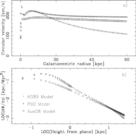
Figure 4: The three Galactic gravitational models are depicted in two different manners here to illustrate their properties and differences. The top panel (a) shows the circular velocity for a range of Galactocentric radial positions in the plane of the Galactic potential. The bottom panel (b) depicts modulus acceleration in increasing height from the plane.

3.2 Initial conditions and integration method

Once we have our assumed Galactic potential, which is in cylindrical coordinates, $\Phi\left(r,\phi,z\right)$, the progenitor pulsar systems must be given some initial Galactic position, $R_{\rm init}$, selected randomly from a given distribution. The most straight forward distribution is to assume a thin disk with some maximum height and radius. This simple method allows the system to relax over time into a similar distribution to the observed stellar number density distribution in height with respect to the plane (see distributions given in Sun & Han 2004). However, as shown in Section 4.1 this overestimates the number of systems (in this case pulsars) found in the central region – the deficiency of observed pulsars within the central region is believed to be a real lack of pulsars and not caused solely by observation selection effects (Lorimer et al. 2006). However, Lorimer et al. (2006) caution readers that more observations are required to provide a definitive result.

To combat this over density within the central regions a preferred option is to use the distribution of SN remnants developed in Paczynski (1990):

$$P(R_{\rm init})dR=a_{\rm R}\left(R_{\rm init}/R^{2}_{\rm exp}\right)\exp{\left(-R_{\rm init}/R_{\rm exp}\right)}dR\,,$$ (31)

where $R_{\rm exp}=4.5$ is simply an exponential scale length of the radial distribution and $a_{\rm R}$ is a constant of integration equal to $1.0683$ over $R=0\rightarrow 20~{}$kpc. A third option is to use the distribution derived by Yusifov & Kucuk (2004; their Equation 17) from observations of OB type Population I stars:

$$P(R_{\rm init})dR=a_{\rm R}\left(R_{\rm init}/R_{\odot}\right)^{4}\exp{\left(-b\frac{R_{\rm init}}{R_{\odot}}\right)}dR.$$ (32)

If OB stars are assumed to be the progenitors of NSs then this can be taken as the Galactic pulsar progenitor birth radial distribution. Here $a_{\rm R}\sim b^{5}/24\sim 606$ (for $0\geq R_{\rm init}\geq 20~{}$kpc). We utilise all three radial distributions – thin disk, Paczynski (1990) and Yusifov & Kucuk (2004) – in our models to generate birth locations. However, because the Paczynski (1990) distribution has had much use in the past we assume this to be our standard description.

In terms of the initial distribution of systems in height from the plane we simply assume a uniform distribution with maximum height of $|z_{\rm maxi}|$. Systems over time relax outwards in $|z|$ and such a simple initial $|z|$ distribution compares well to those favoured in Sun & Han (2004). Furthermore, according to Paczynski (1990) as long as the systems are born relatively close to the Galactic plane (few hundred parsec) the initial distribution in $|z|$ for energetic populations is redundant. In the future the initial spatial distribution will contain spiral arms, similar to that completed within Faucher-Giguere & Kaspi (2006) who suggest that because Galactic arm structure is visible in large observational surveys it is necessary for any realistic pulsar population synthesis simulation to model this structure.

Once a position is found for a system an initial velocity is simply calculated from the (estimated) Galactic gravitational potential at that point. With knowledge of the position and space velocity the next step is to solve four coupled equations of motion to evolve the system position forward in time. These are (Paczynski 1990):

$$\frac{dR}{dt}=V_{\rm R},~{}\frac{dz}{dt}=V_{\rm z},~{}\frac{dV_{\rm R}}{dt}=-\frac{\partial\Phi}{\partial R}+\frac{L^{2}}{R^{3}}~{}{\rm and}~{}$$ (33)

$$\frac{dV_{\rm z}}{dt}=-\frac{\partial\Phi}{\partial z}.$$

These four equations are found by calculating the acceleration in $R$, $\phi$ and $z$ ($V_{\rm R}~{}{\rm and}~{}V_{\rm z}$ are velocities in $R$ and $z$ respectively) induced onto a test particle by the gravitational potential. Assuming an axisymmetric potential around $z$ produces constanst angular momentum, $L$, felt by a test particle. To integrate forward in time a fourth order Runge-Kutta integration routine is used, similar to that used by Paczynski (1990) and Lorimer et al (1993).

It is now possible for us to evolve the complete Galactic orbital evolution of a system of interest. If a SN event occurs and the system is not disrupted the velocity injected into the system by a SN, calculated within bse, is simply vectorially added to the known Galactic velocity of the system centre of mass at the time of the SN. If the system is disrupted the run away velocities of the two stars – as calculated in Section 2.2 – are, again, vectorially added to their previous Galactic velocity (that of their system of origin). In this way we are able to follow the complete Galactic orbital history of a system (star or binary), even if it passes through two SNe and with (or without) binary disruption. Because we assume no interaction between orbiting systems we are able to evolve each system separately, one after another (or in parallel). A beneficial consequence resulting from this assumption is that binkin is faster to run than other dynamical codes, such as typical N-body codes (McGlynn 1984). Of course, if one is dealing with compact stellar clusters dynamical interactions between the stellar components are very important to follow.

4 Pulsar population statistics

We now describe the results of a series of population synthesis calculations that utilise our binpop and binkin modules to follow the stellar/binary and kinematic evolution of a population of binary stars to produce artificial Galactic pulsar populations. The primary aim of this section is to predict scale heights and other kinematic characteristics for populations of pulsars, firstly assuming that all pulsars can be detected. We also compare the kinematics of our model pulsar populations with available kinematic tracers found from pulsar survey observations (such as those produced in Yusifov & Kucuk 2004; Lorimer et al. 2006 and Hobbs et al. 2005). For now we hold back from making direct statistically significant comparisons as this requires modelling of selection effects which will be covered in detail in a companion paper (the binsfx component as mentioned in Section 1). Here we focus more on showing how modifying certain parameters affects the final pulsar population kinematics, in terms of scale heights and space velocity distributions.

Table 1: A summary of the binkin models used within this paper and their main assumptions. The first column provides a label for each model. This is followed by the assumed Galactic radial distribution of pulsar birth locations, $R_{\rm init}$, where Paczynski stands for the distribution suggested by Paczynski (1990; see our Equation 31), Flat is the flat distribution described in Section 3.2 and Yusifov & Kucuk is the birth distribution suggested in Yusifov & Kucuk (2004; see our Equation 32). The third column gives the Galactic gravitational model used (see Section 3.1). The next column is the maximum height with respect to the Galactic plane, $|z_{\rm max}|$, that we consider for our pulsar distribution and scale-height calculations, followed by our assumed value of the SN kick dispersion, $V_{\sigma}$. Note that Model G evolves a population of single stars while all other models start with a population of binaries.

Model	$R_{\rm init}$ distribution	$\Phi$	$|z_{\rm max}|$	$V_{\sigma}$
A	Paczynski	P90	$10~{}$kpc	190
B	Flat	P90	$10~{}$kpc	190
C	Yusifov & Kucuk	P90	$10~{}$kpc	190
C2	Yusifov & Kucuk	P90	$2~{}$kpc	190
C3	Yusifov & Kucuk	P90	$20~{}$kpc	190
D	Paczynski	KG89	$10~{}$kpc	190
E	Paczynski	Xue08	$10~{}$kpc	190
F	Paczynski	P90	$10~{}$kpc	550
G	Paczynski	P90	$10~{}$kpc	265

The first step is to evolve a population of binaries within binpop. For this we proceed using our favoured model from Paper I (Model Fd). This sets choices for binpop stellar and binary evolutionary parameters of: solar metallicity $Z=0.02$; a maximum possible NS mass of $3~{}M_{\odot}$ and $\alpha_{\rm CE}=3$. It also sets the following parameters governing pulsar evolution: $\tau_{\rm B}=2000~{}$Myr; $k=3000$; no propeller evolution; the initial pulsar period and magnetic field parameter selections linked to the strength of the SN velocity kick; the angular momentum accreted by the pulsar is variable; no electron capture SNe; and no beaming of pulsars (see Section 2.1 and Paper I for details). SN kicks using the bse prescription are given to NSs (see Section 2.2), while to keep the required number of models down to a minimum we only use the curvature radiation death line model (Harding, Muslimov & Zhang 2002). Unless otherwise stated we take $10^{7}$ binary systems with initial parameters selected in the same manner as within Paper I and with the limits of $5-80~{}M_{\odot}$ for primary mass, $0.1-80~{}M_{\odot}$ for secondary mass and $1-30\,000~{}$days for orbital period. The Galactic age is assumed to be $10~{}$Gyr. Each binary is evolved to this age and for those that create pulsars the evolution history e.g. SN occurrence times and velocities, is saved as input for binkin.

The next step is to take each of the binpop binaries and follow their corresponding kinematic evolution in binkin. For each binary a random birth age is assigned and the evolution followed from this age up to the age of the Galaxy. For this we begin by defining a standard model which we will call Model A. This uses the Paczynski (1990) distribution for setting the initial Galactic radial positions of the binaries (see Equation 31) with a maximum initial height off the plane of $|z_{\rm maxi}|=75~{}$pc. It also assumes the P90 form of the Galactic potential (see Equations 26 and 27) and sets $V_{\sigma}=190~{}$km s^-1 (used within binpop) as the dispersion of the SN velocity kick distribution. Further models arise due to variations of these choices and are listed in Table 1.

For each model we examine the scale heights for a range of pulsar systems. These are given in Table 2. We take the scale height to be that distance in $|z|$ for which the number of stars within that distance is $63\%$ ($\sim$ twice the e-folding distance) of the entire population. The most prolifically observed pulsar system is what is known as a standard pulsar. Here we define a standard pulsar as one which satisfies

$$\log{B}\geq-2.5\times\log{P}+8.1.$$ (34)

This equation artificially divides the ‘standard’ pulsar ‘island’ from all other radio pulsars in the $B-P$ diagram (see Paper I). We define a MSP to be a pulsar spinning more rapidly than $P=0.02~{}$s. All other pulsars bridge these two pulsar types – islands within the $P\dot{P}$ plane (see also the description given in Paper I). We also distinguish between binary and isolated pulsars. It is possible to compare our model results in a limited manner to observations. To do this we make use of the ATNF Pulsar Catalogue which provides us with $\sim 1610$ Galactic plane pulsars (we ignore pulsars from the catalogue that have any association with another object, for example with a globular cluster or external galaxy). Approximately $1550$ of these are isolated. Only $15$ standard pulsars are found in binary systems within the Galactic disk. Of the total observed pulsars there are $65$ MSPs of which $19$ are isolated. We show the scale heights of the catalogue pulsars within Table 3.

The radial distributions of Galactic pulsars resulting from our set of models are shown in Figure 5 (left-hand side panels). We also compare a subset of the models in more detail in Figure 6 and include a comparison to the initial distributions used in the models and also the pulsar distribution suggested by Yusifov & Kucuk (2004) which is based on observations. We also explore the pulsar population 3D space velocity distributions. These are shown in the right-hand side panels of Figure 5 for the models in Table 1.

Our results are analysed in more detail in four parts. In Section 4.1 we examine the effect of varying the assumed pulsar birth radial distribution. This analysis makes use of Models A, B and C. Within Section 4.1 we also consider how modifying the target area considered (the ‘observable’ Galactic area) in our scale height calculations affects the scale height values of pulsars produced in Model C. This is completed with the use of Models C2 and C3. Section 4.2 analyses different forms of the Galactic gravitational potential by comparing Models A, D and E pulsar scale heights, final radial distributions and final velocity distributions. We then consider the effect of varying the assumed SN velocity kick distribution with Models A, F and G in Section 4.3. Finally, after examining differences in bulk pulsar properties, we explore in detail the MSP population of Model C in Section 4.4. We make use of our MSP analysis to further investigate the effect of model assumptions such as the initial scale height, Galactic age and the number of systems evolved.

Table 2: Model scale heights for a range of pulsar types in the Galaxy.

		Model	A	B	C	D	E	F	C2	C3
Type
	Both		$1.39$	$1.49$	$1.25$	$1.33$	$2.58$	$1.93$	$0.58$	$1.40$
All	Isolated		$1.43$	$1.53$	$1.30$	$1.37$	$2.64$	$1.93$	$0.59$	$1.46$
	Binary		$0.96$	$1.10$	$0.79$	$0.91$	$1.98$	$2.00$	$0.46$	$0.83$
	Both		$1.43$	$1.53$	$1.30$	$1.36$	$2.63$	$1.93$	$0.59$	$1.45$
Standard	Isolated		$1.43$	$1.53$	$1.30$	$1.37$	$2.64$	$1.93$	$0.59$	$1.46$
	Binary		$0.73$	$0.85$	$0.59$	$0.71$	$1.68$	$1.58$	$0.38$	$0.61$
	Both		$1.00$	$1.15$	$0.82$	$0.95$	$2.04$	$2.02$	$0.47$	$0.88$
All MSPs	Isolated		$1.76$	$1.67$	$1.76$	$1.49$	$2.90$	$2.33$	$0.60$	$2.21$
	Binary		$0.99$	$1.14$	$0.82$	$0.94$	$2.03$	$2.02$	$0.47$	$0.87$

Figure 5: Left panels: theoretical radial distributions of pulsars for a range of models. All model radial distributions are normalised to Model A. Right panels: theoretical space velocity distributions for the same range of models. The velocity distributions depicted here represent the pulsar population space velocities with respect to the Galactic centre. The solid line in the bottom-right panel depicts the 3D space velocity distribution of young pulsars derived from observations (Hobbs et al. 2005). All velocity distributions are normalised to unity.

4.1 Initial distributions and target area

To begin with we focus on Model A. We note that unless otherwise specified, when calculating scale heights we consider only pulsars located within the Galactic region defined by $|z|\leq|z_{\rm max}|~{}$kpc and $r=\sqrt{x^{2}+y^{2}}\leq 30~{}$kpc. Firstly comparing the scale heights of the isolated and binary pulsars we see that as expected (see Section 1) it is the isolated pulsars which have the greatest scale height when considering all pulsars. It is also no surprise that the scale height of the complete population (top row of Table 2) is closely aligned with the isolated pulsar scale height. This is because 91% of pulsars in Model A are isolated at the end of the simulation (even though all stars are initially in binaries). When considering only standard pulsars the domination of the isolated component is even greater: 99% of standard pulsars are isolated. However, the tables are turned when we look at the MSP population: the binary MSP population makes up 99% of all MSPs within Model A (a greater percentage than what is observed, however, see Section 4.4.1 for further discussion on this point). These relative numbers explain why in Table 2 the scale height of standard pulsars is insensitive to standard binary pulsars, and the same can be said for the total MSP scale height compared to isolated MSPs.

For the binary pulsars we find that the standard pulsar population has a lower scale height than for the MSP population. This suggests that on average binary MSPs receive greater post-SN recoil velocities than their standard binary pulsar counterparts. The reasons for this were alluded to in Section 1 but we reiterate them here (see also the findings of Stollman & van den Heuvel 1986; Bailes 1989). Basically, the very existence of an MSP relies on the occurrence of mass-transfer on to the NS which in turn requires a close binary. Such a binary will have a greater binding energy than the equivalent standard (wider) binary pulsar and can therefore survive a greater SN velocity kick as there is more energy to overcome for disruption. As a result it is possible for the proto-binary MSP system to be given a faster recoil velocity (with respect to the systems initial CofM). The isolated MSP population scale height also increases compared to the entire isolated pulsar population. Again this is not surprising given the model isolated MSP formation scenario as addressed in Paper I and within Section 1. Owing to the SN that produced the NS progenitor of the MSP, and the SN of the companion star that disrupted the system, isolated MSPs can receive greater recoil velocities than any other pulsar population – hence the largest population scale height (this formation mechanism is also discussed further in Section 4.4).

To measure what effect the initial Galactic birth distribution has on the final model pulsar population we compare Models A, B and C. These models assume the birth distribution of Paczynski (1990: from the observed distribution of SN remnants), a uniform thin disk, and the birth distribution of Yusifov & Kucuk (2004: derived from observations of OB stars), respectively. The final radial distributions (at a Galactic age of $10\,$Gyr) for the pulsars in these models are compared in the upper-left panel of Figure 5. Both Models A and C have distributions that peak away from the Galactic centre (reflecting their initial distributions). However, the peak of Model A is shallower and the distribution is more extended than Model C. We note that the number of pulsar systems ‘observed’ in Model C is higher than in Model A (by a factor of $\sim 1.1$). For Model B we find that the pulsar radial distribution peaks at the Galactic centre and then decays with increasing radius. The space velocity distributions for the pulsars in the three models are compared in the upper-right panel of Figure 5 and we see that there is no discernible difference.

The relation of the final pulsar radial distribution to the assumed birth distribution of binaries can be seen in Figure 6 for Models A and C. Here all distributions are normalised to unity to aid comparison of the peak position and distribution shapes. We see that the birth distribution of Model A is broader than for Model C and this is reflected in their final shapes. However, the width of the distribution increases with time in both cases, while the peak of the distribution moves in towards the Galactic centre, which is a typical effect of Galactic potentials (Sun & Han 2004). Initially Model A peaks at a radius of $4.5\,$kpc which moves inwards to a radius of $3.9\,$kpc at $10\,$Gyr. For Model C the peak moves from $5.0\,$kpc to $4.5\,$kpc.

In Figure 6 we also compare the model distributions to the distribution of an observed sample of pulsars presented by Yusifov & Kucuk (2004). We note that at this stage we are not including selection effects in our models so a direct comparison with observations is not possible. However, comparison with the Yusifov & Kucuk (2004) sample, which includes selection effects somewhat by being limited to pulsars with $\dot{P}>10^{-17}~{}$s s^-1, can still provide a meaningful guide to discerning between our models. Although not included in Figure 6 we can see immediately that Model B is an unrealistic model of the Galactic pulsar population. The apparent deficit of observed pulsars in the inner region of the Galaxy can not be reproduced by assuming all binaries are born in a uniform thin disk – we require a paucity of pulsars to be born in the central region of the Galaxy when attempting to match observations (similar to Paczynski 1990; Sun & Han 2004). This lack of observed inner Galactic pulsars may be due to the high electron density in this region of the Galaxy and therefore larger scattering of the pulse signal, however, the latest observations do suggest an intrinsic scarcity of central pulsars (Lorimer et al. 2006). Model A provides a good comparison to the observed radial pulsar distribution for the inner regions of the Galaxy but has too many pulsars and is too extended beyond $\sim 4~{}$kpc. In terms of shape, Model C best represents the observations. However, Model C peaks further from the Galactic centre by $1-1.5\,$kpc. This suggests that the ideal initial distribution would of the form derived by Yusifov & Kucuk (2004) from observations of OB stars but scaled so that the distribution peaked at a radius of $\sim 4\,$kpc.

The scale heights for Models A, B and C can be compared in Table 2. We see that Model B has systematically the largest scale heights while Model C has the smallest. However, the trends observed for Model A – the relative scale heights of the various pulsar populations – are consistent across the models

We next demonstrate what effect modifying the Galactic region of interest has on Model C by considering pulsars only out to $|z|=2~{}$kpc in Model C2 and out to $|z|=20~{}$kpc for Model C3 (as opposed to $|z|=10~{}$kpc for Model C). We find that reducing the height of our ‘Galaxy’ by a factor of five approximately halves the calculated scale heights for all pulsar populations. On the other hand, doubling the height considered does not significantly affect the calculated scale heights (except perhaps the isolated MSP population which suffers from small number statistics). However, it does not appear to greatly affect the relative scale heights of pulsar sub-populations and certainly does not switch any trends noted in the models. Beyond this limit only the results of highly energetic systems may still vary. Therefore, factors which limit the region of the Galaxy observed (or considered), such as the numerous selection effects which occur in radio pulsar observations, can modify the underlying pulsar population scale heights within $|z|<10~{}$kpc of the Galactic plane (as discussed by many works including Taylor & Manchester 1977 and Narayan & Ostriker 1990). We note that in terms of Galactic pulsar observations there is the limit of $\sim 1.75~{}$kpc beyond which dispersion measure distance estimates of pulsars break down (see Manchester et al. 2005).

We now have Model C, a suitable model for which we may compare pulsar scale heights to observations (the latter values are given in Table 3). Model C2 is roughly consistent with the observed scale heights, although on average the model values are greater than the observed values. The trends when considering all pulsars are similar but this breaks down for the MSP population where the model predicts a greater scale height for isolated MSPs than for binary MSPs which is opposite to the observed MSP scale heights (although, see Section 4.4.1). This is, however, consistent with our previous simple analysis in Section 1 from the binary disruption formation mechanism of isolated MSPs. Another difference between Model C2 and observations is the relative number of isolated to binary MSP systems. In Model C2 $\sim 99\%$ of MSPs are found within a binary system while a direct observational comparison shows $\sim 70\%$ of Galactic disk MSPs in binary systems. These two differences between our model and observations indicate that our mechanism for producing isolated MSPs – binary disruption in a SN event – can not be the sole (or even dominant) production mechanism. We explore this line of thought further in Section 4.4.

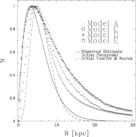
Figure 6: Theoretical radial distributions of pulsars for a select few models all normalised to unity. Here we restrict ourselves to only consider those pulsars with $\dot{P}>10^{-17}~{}$s s^-1 which compares to the observed sample used by Yusifov & Kucuk (2004: solid line). Also provided is the initial radial distribution given in Paczynski (1990: dotted line), which is used in Models A, D and E, and the initial radial distribution of Yusifov & Kucuk (2004: dash dotted line) used in Model C.

Table 3: Observed scale heights (in kpc) for different types of pulsars. We have not taken account of selection effects when calculating these values. Standard pulsars are those pulsars which satisfy Equation 34, while MSPs are those pulsars which have spin-periods $P\leq 0.02~{}$s. We note that there is uncertainty in some of these numbers owing to small number statistics and the clumpy distribution of the pulsars. For example, there are only $19$ isolated MSPs and the difference in height between the 12th and 13th most distant (in terms of height from the plane) is $0.07~{}$kpc while the average distance between the first twelve is $0.02~{}$kpc.

Type	All	Standard	MSP
Both	0.40	0.39	0.41
Isolated	0.41	0.39	0.26
Binary	0.38	0.17	0.48

4.2 Model Galactic gravitational potentials

We now explore what effect modifying the assumed Galactic gravitational potential has on the pulsar scale heights and final distributions (radial and space velocity). Model D assumes a potential of the form described by the KG89 model (Equation 21). The scale heights of Model D are all slightly less than their Model A counterparts which used the P90 model. This suggests that over time stellar systems may diffuse less efficiently in Model D than in Model A. Figure 4 gives some indication of the cause of this difference. The lower panel of provides the model Galactic gravitational force towards the plane with respect to the height above the plane. We see that above a height of $|z|\sim 1~{}$kpc the KG89 model has a slightly greater attractive force than the P90 model. However, for the inner regions the situation is reversed and indeed if we calculate the scale heights for pulsars with $|z|<1~{}$kpc, we find that the scale height behaviour for Model D relative to Model A is also reversed. As shown in Figures 5 and 6 the radial distribution does not differ greatly between Models A and D: small differences to note are that the distribution of Model D decays more rapidly than Model A while Model D contains less pulsar systems within $10~{}$kpc of the Galactic plane. The velocity curve of Model D does not change greatly from Model A as there is only a small increase in systems with space velocities at the lower end of the distribution, perhaps reflecting the rapid decay in circular velocity of Model D with respect to Model A (see Figure 4).

Model E assumes the Galactic gravitational potential of Xue08 (Equations 28 to 30). This model shows a large increase in scale height values compared to both Models A and D. The reason for this can once again be seen from Figure 4 which shows that the Xue08 Galactic gravitational model can not retard the movement of systems out of the Galactic plane as effectively as the P90 (Model A) or KG89 (Model D) models. Figure 5 shows that the number of systems retained by Model E within $|z|\leq 10~{}$kpc is less than within both Models A and D. The 3D space velocity curves of Models A, D and E all peak at roughly the same value but the Model E distribution possesses a much steeper slope either side of its peak value. The flatness of the rotation curve assumed in Model E, depicted in Figure 4, causes such a narrow distribution in velocity space. Model E highlights the importance of the assumed Galactic gravitational potential in modelling Galactic population kinematics (as also discussed by Kuijken & Gilmore 1989, Dehnen & Binney 1998 and Sun & Han 2004).

4.3 Kicks

Considering the uncertainty involved in the true form of the distribution of kick speeds given to NSs at birth (as mentioned in Section 2.2.1) we next investigate how changing the dispersion of the assumed Maxwellian distribution affects our results. Recalling that Model A used $V_{\sigma}=190~{}$km s^-1 we first compare with Model F which uses $V_{\sigma}=550~{}$km s^-1 as an extreme illustration. We see from Table 2 that the scale heights in Model F are much greater than in Model A, with increases by as much as a factor of 2. While it is expected that pulsars can move further from the galactic plane in Model F it also means that more objects escape from the Galaxy: the number of pulsars in Model F within $10\,$kpc of the plane decreases by a factor of 10 compared to Model A. This decrease in numbers can skew the expected outcomes and is evident when looking at the radial distributions in Figure 5. For example, less binary systems are kicked out of the $|z|\leq 10~{}$kpc Galactic region than isolated pulsars – owing to binaries being heavier on average and the binary orbit absorbing a fraction of the energy injected by the kick – so we find in Model F that binary pulsars have a greater scale height than isolated pulsars (the opposite to Model A). This is not the case for MSPs although the difference between the isolated and binary MSP scale heights has decreased compared to Model A. We note that the ratio of standard isolated pulsars to standard binary pulsars is an order of magnitude greater for Model F than for Model A owing to a greater incidence of binary disruptions in Model F. Therefore, as established in previous works (e.g. Taylor & Manchester 1977; Hills 1983), the assumed SN kick velocity is an extremely important factor, especially when comparing model pulsar kinematics to observations.

When examining the resultant radial distribution in Figure 5 we find that Model F is much broader than Model A – an intuitive results owing to the increased distance that the pulsars move – and certainly Model F is not a good representation of the observed distribution (not that it was expected to be). Comparing the space velocity distributions of Models A and F in Figure 5 it is surprising to see the relatively high number of pulsars in Model F that are traveling at the distribution peak speed ($\sim 250~{}$km s^-1). This population with similar velocities includes isolated and binary pulsars. We remind the reader that when discussing the velocity distribution here we mean the actual velocity each system has with respect to the Galactic centre – we do not account for the local standard of rest (solar motion).

In Figure 5 we also compare the 3D space velocity distributions of Models A and F with the 3D space velocity distribution derived by Hobbs et al. (2005) from pulsar observations. An important distinction to make is that the Hobbs et al. (2005) sample was restricted to pulsars with characteristic ages $<3~{}$Myr. Thus, it is intended to be a distribution of pulsar birth velocities and was used by Hobbs et al. (2005) to suggest that $V_{\sigma}=265~{}$km s^-1 in the SN velocity kick distribution. By comparing this with our models we can gauge the effect that the Galactic potential and binarity have on the form of the pulsar velocity distribution as the population evolves.

Comparing the Model A pulsar velocity distribution (at a population age of $10\,$Gyr) with the Hobbs et al. (2005) birth velocity distribution shows changes in the peak (shifted to lower velocity in the model) and shape. The shift of the peak can be mostly attributed to the difference in the average age of the two pulsar populations and the low dispersion value assumed in the Model A velocity kick distribution. The age difference allows fast moving systems in Model A to have time to leave the Galaxy and thus be culled from the final velocity distribution. Also, over time, the pulsar velocities are retarded by the Galactic potential which shifts the final pulsar velocity distribution to lower velocities. In terms of shape we find that Model A is a more focussed distribution – the model peak is more acute and the distribution as a whole is narrower. This difference is likely due, in part, to the binding energy of the host binaries impinging on the SN velocity kick (as discussed in Hills 1983 and Bailes 1989) and causing a greater number of systems to have similar final space velocities than otherwise. Disruptions triggered primarily by mass loss will act to increase the proportion of low velocity pulsars while the absorption of large kick velocities by the binary binding energy may also skew the distribution to smaller final pulsar velocities. This narrowing of the model pulsar velocity distribution compared to the observed distribution has been found in other works, most notably that of Dewey & Cordes (1987). They attributed the difference to errors in pulsar distance measurements, which will broaden the distribution, and that non-Maxwellian processes may be more important in producing pulsar velocities than their models assume (that is, nascent NS receiving a kick selected from a Maxwellian distribution with $<V>=90~{}$km s^-1). It appears that the difference between the velocity distribution of models and observations results from a combination of the selected pulsar population used to derive the observed pulsar velocity distribution (see Hobbs et al. 2005), errors in pulsar velocity and distance measurements, and the binding energy of host binary systems affecting the resultant pulsar run-away velocity.

To remove the binary orbit effect and highlight the effect of age evolution on the pulsar velocity distribution we have created Model G which evolves a population of single stars according to the Galactic setup described for Model A but with $V_{\sigma}=265~{}$km s^-1. With every system evolved within Model G being isolated from birth we are now able to compare the resultant velocity distribution of a population of pulsars which receive uninhibited SN kick velocities drawn directly from the suggested Hobbs et al. (2005) SN kick distribution. We now see in Figure 5 that the distribution closely resembles the Hobbs et al. (2005) distribution in shape but is shifted to lower velocities. The final pulsar distribution is best fit by a Maxwellian distribution with $V_{\sigma}=140~{}$km s^-1.

4.4 Millisecond pulsars

Table 4: Scale heights (in kpc) of MSPs and their companions for Model C (see Section 4.4.1) and its variants (see Sections 4.4.4 and 4.4.5).

Model	C	C${}^{{}^{\prime}}$	C${}^{{}^{\prime\prime}}$
MSP-MS	$0.74$	$0.75$	$0.74$
MSP-WD	$0.83$	$0.84$	$0.86$
MSP-NS	$1.96$	$1.93$	$2.06$
MSP-BH	$0.11$	$0.13$	$0.10$
Isolated MSP	$1.76$	$1.76$	$1.61$
Ablation	C	C${}^{{}^{\prime}}$	C${}^{{}^{\prime\prime}}$
Binary MSP	$0.87$	$0.87$	$0.91$
Isolated MSP	$0.75$	$0.75$	$0.77$

In Paper I we were primarily interested in the production of MSPs within the $P$-$\dot{P}$ diagram. We now continue our exploration of the MSP population by examining in more detail the Galactic MSP distributions and in particular focussing on the behaviour of isolated MSPs and those with MS star, WD, NS or BH companions. In doing this we focus solely on Model C. To begin, we extend our evaluation of scale heights in Table 2 with those of the MSP populations (given in Table 4 and discussed in Section 4.4.1). The scale heights in Table 4 are supplemented by Figure 7 which provides the scale height for each MSP population as a function of Galactocentric radius. Also shown is the Galactic $x$ and $z$ parameter space of MSPs: for all MSPs (see Figure 8) and those that reside above a magnetic field cut-off (see Figure 9). The population of MSP-BH binaries is then discussed in detail within Section 4.4.2. We then look at the MSP population recoil velocities and space velocities in Section 4.4.3 and make some limited comparisons to previous work and observations. To further our investigation into how different model assumptions affect our pulsar population kinematics, we modify Model C, our favoured model thus far, to account for: a greater birth $|z_{maxi}|$ range (Model C${}^{{}^{\prime}}$ in Section 4.4.4); a greater age of the Galaxy (Model C${}^{{}^{\prime\prime}}$ in Section 4.4.5); and a higher resolution sample (in Section 4.4.6).

4.4.1 Model C MSP scale heights and Galactic spatial properties

Looking at the scale height values in Table 4 for Model C we see that as expected the binary MSP population with the greatest scale height is the MSP-NS systems, in which two SNe kicks occur. These double compact systems, however, are much rarer than the MSP-MS or MSP-WD systems and therefore the results are less statistically significant. The relative numbers of MSP-NSs compared to MSP-WD systems (the largest MSP population) is $0.003$. For MSP-MS systems (the second most numerous MSP population) the relative number is $0.044~{}$per MSP-WD system. We find similar scale heights for the MSP-MS and MSP-WD systems although the former are systematically smaller owing to the population being younger on average. Recently there have been suggestions that asymmetric mass-loss during the asymptotic giant branch phase (Spruit 1998) give rise to WD recoil velocities of the order of a few ${\rm km}\,{\rm s}^{-1}$ (Fellhauer et al. 2003). Such kick velocities have been raised a possible explanations of the apparent deficit of WDs in open clusters (Fellhauer et al. 2003) and the radial distributions of WDs in globular clusters (Heyl 2007; Davis et al. 2008). Currently we do not include this possibility in our models but note that it would presumably lead to a modest increase in the MSP-WD population scale height.

MSP-BH systems are found to have a small Galactic scale height. This arises due to the orbital parameters required in order to form these systems which we examine in further detail below (see Section 4.4.2). Also, we remind the reader that we currently assume BHs do not receive kicks during their formation. As shown in Tables 2 and 4 the isolated MSP population has a scale height of $1.76~{}$kpc. These MSPs emerge from disrupted binary systems and although the kick at the time of disruption may be large it is not the MSP which is exploding at that point. Therefore the MSP is considered by our kick routine to be the secondary star which, as shown in Section 2.2.3, receives (on average) only a small increase in momentum. This results in the lower scale height of isolated MSPs compared to MSP-NS binary systems (albeit only slightly less than the MSP-NS value). Furthermore, we note that for the binary system to survive the first SNe, allowing mass transfer onto the progenitor MSP, the resultant velocity kick at this point must be relatively small (we find $V_{\rm kick}$ of approximately $80~{}$km s^-1 or less). This is in accordance with many other population synthesis works, including Stollman & van den Heuvel (1986), Iben, Tutukov & Yungleson (1995) and Ramachandran & Bhattacharya (1997).

Previous results shown in Section 4.1 placed doubt on isolated MSPs formed via the disruption of binary systems being the sole ‘type’ of isolated MSPs – there must be another formation mechanism. One such mechanism that exists in the literature is the ablation model (Eichler & Amir 1988; Ruderman et al. 1989) based on observations such as those of van Paradijs et al. (1988). Here the assumption is that the MSP is produced as a result of mass-transfer from a MS companion in what would be a low-mass X-ray binary. Then at some point the mass of the MS star becomes low enough that it is destroyed, or ablated, by the highly energetic radiation flowing from the rapidly spinning pulsar (van Paradijs et al. 1988; Tavani 1992). We calculate that the timescale for the destruction of the MS companion star in this manner should take of order $\sim 5~{}\rm{Myrs}$ once the companion is below a mass of $\sim 0.02\,M_{\odot}$ (see Appendix A). Thus we propose a simple model to belatedly estimate the impact of ablation on our results where we assume that any MSP with a MS companion of mass less than $0.008M_{\odot}$ (to be on the safe side) is in fact an isolated MSP. With the inclusion of ablation we find that the percentage of isolated MSPs increases from 1% to 36%. This new value is in rough agreement with observations where it is estimated that one third of the MSPs are isolated (Huang & Becker 2007). Iben, Tutukov & Tungleson (1995) similarly found good agreement with observations for binary to isolated ratios when assuming ablation of MSP companions. We see from the last two rows in Table 4 that the isolated and binary MSP populations now have comparable scale height values (in fact the isolated scale height is now slightly the lower of the two). Therefore the kinematics of the binary and isolated MSP populations are now similar. This last point is actually consistent with the observations of MSPs, which via statistical arguments show no difference in binary and isolated MSP kinematics (Lorimer et al. 2007). From this simple test we see that the low mass companions to MSPs do occur and that the ablation process deserves serious consideration in future models.

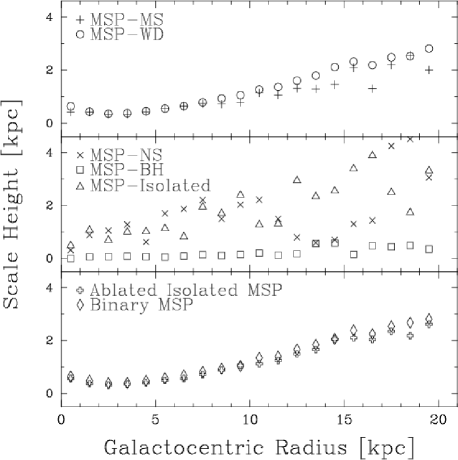
Figure 7: The radial variation of pulsar scale heights for a range of MSP populations in Model C.

In Figure 7 we show how the scale heights of the MSP populations vary with Galactocentric radius. We note that the region of the Galaxy where the populations are most numerous is between $4-6~{}$kpc from the Galactic centre. The top panel of Figure 7 depicts the similarity of MSP-MS and MSP-WD kinematics. It is only out beyond $\sim 13~{}$kpc that the two populations diverge, and this is only due to low number statistics which begin to plague the MSP-MS results. Low number statistics have a much greater influence in the middle panel of Figure 7. For example, the highest number of systems in a radial bin ($1~{}$kpc in width) for the MSP-NS population contains $39$ systems while the lowest only $3$. The MSP-NS and isolated MSP systems have similar scale heights throughout the majority of the Galaxy (after accounting for statistical uncertainty) and systems can be found far from the plane. The MSP-BH systems on the other hand are all found close to the Galactic plane. When accounting for the ablation of MSP companions we find a very similar distribution of binary and isolated MSPs throughout the entire Galaxy.

It is also interesting to compare the spatial Galactic $x-z$ distributions of the MSP populations. This is shown in Figure 8 for the Galactic $xz$-plane and emphasises what we have already seen in Table 4 and Figure 7: isolated MSPs and MSP-NS binaries have quite extended distributions (relative to their numbers), MSP-BH systems reside close to the plane and the majority of MSPs are found with WD companions (MSP population numbers relative to MSP-WD systems are given in the lower right corner of each panel). What is surprising in Figure 8 is the large number of MSP-WD systems out to $|z|=10~{}$kpc. This suggests that there may be many MSP-WD systems lost from – but surrounding – the Galaxy. We next investigate the result of imposing a limited selection effect on the MSP population where we only consider pulsars that have $B>6\times 10^{7}~{}$G. This magnetic field value is a suggested limit (Zhang & Kojima 2006) of the required field strength to turn on (or off) the pulse mechanism (see Paper I). Figure 9 shows the field strength limited MSP population and the result in comparison to Figure 8 is dramatic. The entire MSP-BH population now disappears, which is also almost the case for the MSP-MS population where only two systems are left. The relative numbers of both isolated MSPs and MSP-NSs have now increased compared to the MSP-WD systems (see values on Figures 8 and 9). Clearly many MSPs in Model C accrete enough mass to cause a large decay in the magnetic field. In particular every pulsar within a MSP-BH system has accreted more than $\sim 0.04~{}M_{\odot}$ of material which is the typical amount of mass it takes for our model pulsar magnetic fields to decay below $B=6\times 10^{7}~{}$G (see Paper I). This is compared to other works which assume $\Delta M>0.1~{}M_{\odot}$ is required for MSP production (e.g. Willems & Kolb 2005).

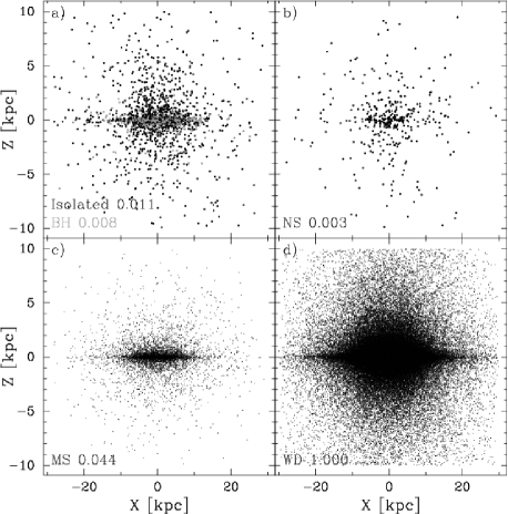
Figure 8: Galactic $x$ and $z$ coordinates for Model C MSP systems within a radius $R=\sqrt{x^{2}+y^{2}}<30~{}$kpc of the Galactic centre and $|z|\leq 10~{}$kpc from the Galactic plane. The bottom left corner of each panel gives the MSP companion type and relative number of that system compared to the MSP-WD systems. Due to their lack of numbers the points for MSP-NSs, MSP-BHs and isolated MSPs are larger than for the MSP-MS and MSP-WD systems.

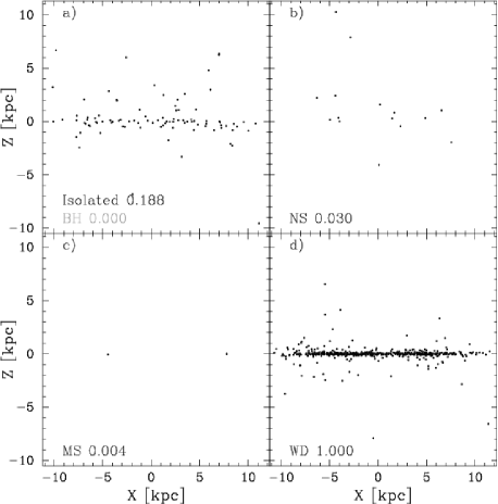
Figure 9: As for Figure 8 but now restricted to include only pulsars that satisfy $B\geq 6\times 10^{7}~{}$G.

4.4.2 Model C MSPs and BHs

Although other works have detailed BH and pulsar binary evolution in varying detail (Narayan, Piran & Shemi 1991; Lipunov et al. 1994; Pfahl, Podsiadlowski & Rappaport 2005; Lipunov, Bogomazov & Abubekerov 2005) we evaluate the accretion history of MSP-BHs and why these systems reside close to the Galactic plane. To place this into context we explore the initial orbital period and initial primary mass (the MSP progenitor and initially the more massive star) parameter space in Figure 10. This figure is also designed to show which systems reside in a range of observable orbital periods (that is orbital periods which would be observed now, if the age of the Galaxy is $10~{}$Gyr). Figure 10 also gives the secondary mass (BH progenitor and initially the less massive star) range for each binary system depicted. What we find in Figure 10 is three distinct groups in both initial orbital period and final orbital period. Each of the three regions have different evolutionary pathways which leave the systems close to the Galactic plane. We now describe these evolutionary pathways. Firstly, however, we note the healthy number of MSP-BH systems (few hundred) produced within our model. This is in contrast to Pfahl, Podsiadlowski & Rappaport (2005) who suggest that BHs with recycled pulsar companions are rare. The primary differences between our model and that of Pfahl et al. (2005) – in terms of BH formation – is their assumption that SN kicks are given to BHs, the assumed evolutionary parameter values within the CE phase and massive star wind mass-loss and accretion. In varying the CE parameters Pfahl et al. (2005) show that $\sim 100$ MSP-BH systems can be produced (with extreme CE parameter choices), however, a favoured model estimates only $5-10$ MSP-BH systems within the Galaxy. This compares well with the number of systems we find with orbital periods less than $\sim 10\,$hr, which is roughly the maximum orbital period limit Pfahl et al. (2005) find for MSP-BH systems. We also include an evolutionary pathway which forms an MSP-BH system that does not include a CE phase, something not considered by Pfahl et al. (2005; who do, however, comment on this scenario).

Those systems which begin their lives with initial orbital periods less than $10\,$days all have an initial primary mass of $M_{\rm 1i}>40~{}M_{\odot}$ and an initial secondary mass of $M_{\rm 2i}>20~{}M_{\odot}$. These systems end with the largest BH masses (around $\sim\,13~{}M_{\odot}$) of all the MSP-BH populations and their orbital periods are grouped near $1000~{}$days. These systems were not found by Pfahl et al. (2005) possibly owing to the inclusion of SN kicks during BH formation. The general evolution pathway of these systems goes as follows. The initial orbital separation is of the order of $80\,R_{\odot}$ or less and the massive primary star evolves to fill its Roche-lobe within a few Myr. This leads to a phase of steady mass transfer lasting $1-2\,$Myr and ending with the primary as a naked helium star with a mass of about $10\,M_{\odot}$. During the phase the secondary accretes approximately 80% of the transferred material with the remainder lost from the system. The orbital separation at this point is typically $200~{}R_{\odot}$ and subsequently increases further owing to winds from the helium star and the now massive secondary. At a system time of $\sim 5\,$Myr the primary undergoes a SN explosion and becomes a NS. We find that velocity kick magnitudes of $V_{\rm kick}\leq 80\,$km s^-1 allow the system to remain bound. Beyond the first SN the secondary evolves quickly and loses a large proportion of its matter in a wind, some of which is accreted by the NS companion. The secondary evolves via a naked helium star phase to explode as a SN and leave a BH remnant. At this point we have an eccentric MSP-BH system which has received one mild SN velocity kick in its lifetime and has typical component masses of 2 and $10-13\,M_{\odot}$, for the NS and BH respectively. The orbital separation is in the range of $1000-4000\,R_{\odot}$ (depending on the precise details of the kick velocity and the mass-loss history).

Those MSP-BH systems with $10<P_{\rm orbi}<100\,$days as seen in Figure 10 end their lives with a large range of BH masses extending from $3~{}M_{\odot}$ through to $11~{}M_{\odot}$ in tight orbits around their MSP companion ($P_{\rm orbf}<20~{}$days). It is this population of MSP-BHs which are most likely to coalesce at and around the age of the Galaxy (similar to Pfahl et al. 2005). Initial primary masses are in the $18<M_{\rm 1i}/M_{\odot}<30$ range and secondary masses are typically $10<M_{\rm 2i}/M_{\odot}<20$. The initial orbital separation ranges from $100-300R_{\odot}$. Early evolution proceeds similarly to that of the previous group: non-conservative mass transfer from the primary to the secondary accompanied by an increase in the orbital separation and ending with the primary as a naked helium star. The primary then undergoes a SN and becomes a NS at a system time of about $8\,$Myr. We find that generally these systems can survive slightly larger SN velocity kicks than the systems described in the previous group. The companion is now a massive MS star ($\sim 30\,M_{\odot}$) and subsequently fills its Roche-lobe while crossing the Hertzsprung Gap. This initiates dynamical-timescale mass transfer leading to a common-envelope phase and the creation of a tight binary comprised of the NS primary ($\sim 2\,M_{\odot}$) and a naked helium star secondary ($\sim 10\,M_{\odot}$). We note that systems in the first group avoid this second Roche-lobe filling event because the secondary is more massive and loses mass in a wind at a greater rate leading to more substantial orbit expansion after NS formation. After emerging from the common-envelope the NS then accretes material from the wind of the companion to become a MSP. This ends when the companion becomes a BH. The final MSP-BH binary will have an orbital separation of less than $10\,R_{\odot}$ and systems such as this may coalesce within a Hubble time.

Figure 10: MSP-BH initial population parameter space of Model C, in particular the initial orbital period and zero-age main-sequence primary star (MSP progenitor) mass. Provided are ranges of the initial companion mass (BH progenitor). Those systems with initial orbital periods, $P_{\rm orbi}>100~{}$days end with final orbital periods $P_{\rm orb}>10000~{}$days. Those with $P_{\rm orbi}<10~{}$days end with $20<P_{\rm orb}<10000~{}$days and those with $10<P_{\rm orbi}<100~{}$days end with $P_{orb}<20~{}$days.

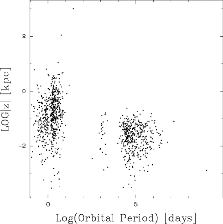
Figure 11: Model C MSP-BH pulsar $|z|-P_{\rm orbf}$ parameter space. There are three distinct groups in final orbital period. The group on the left corresponds to systems with $10<P_{\rm orbi}<100~{}$days, the central group corresponds to systems with $P_{\rm orbi}<10~{}$days and the right hand group corresponds to systems with $P_{\rm orbi}>100~{}$days (see Figure 10).

The MSP-BH systems with $P_{\rm orbi}>100\,$days end with orbital periods of 1000 days or more (see Figure 11 for the final orbital period range). We note that the smallest primary and secondary masses belong to this group. Once again mass-transfer occurs prior to the first SN event but owing to the wider orbit this is initiated later ($\sim 15\,$Myr) than in the previous cases and when the primary is a giant star. The orbital separation when the primary undergoes a SN (to become a NS) is typically $2000-3000\,R_{\odot}$ which means that relatively smaller kicks are required if the system is to remain bound and proceed to become a MSP-BH binary. We find that kicks of the order of 20 km s^-1 or less are necessary (slightly larger if the kick is well directed). After NS formation the secondary is a MS star with mass of approximately $20\,M_{\odot}$. The secondary then evolves off the MS and transfers some material to the NS before ending its life as a BH of mass less than $5\,M_{\odot}$.

The above analysis shows that the most likely MSP-BH systems to be created are those in which the first SN – the only one assumed to impart a velocity kick onto the compact remnant – produces a small velocity kick, which is why these systems are found to hug the Galactic plane as suggested by Narayan et al. (1991). In fact, compared to the other MSP binary populations the MSP-BH systems effectively represent a different kick distribution, in that the distribution of kicks given to systems that remain bound is distinct. As touched on in the evolutionary descriptions this is also true internal to the MSP-BH population, where the effective kick distribution for systems that remain bound is different for each of the three period groupings we identified in Figure 10. This is depicted indirectly in Figure 11. Here we see the MSP-BH height from the Galactic plane and the populations are designated by their grouping in the final orbital period parameter space. Each population has a different scatter in $|z|$, which can be used as an indicator for the average strength of the SN velocity kick. We see that the majority of those small orbital period MSP-BH systems are further off the plane than the extremely long period MSP-BH systems, suggesting that as expected from Bailes (1989), the close binary systems can survive larger kick velocities than the larger binary systems (which was outlined in the evolutionary examples). Only three MSP-BH systems are found beyond $10~{}$kpc from the Galactic plane.

The MSP-BH orbital period distributions as shown in Figure 11 are remarkably distinct and perhaps surprisingly not smeared out by our use of random birth ages. This is due to the vast orbital period differences between these populations and the time scales these populations evolve on. The orbit of MSP-BH binary systems, after the formation of the BH, can only shrink in time owing to gravitational radiation (Landau & Lifshitz 1951; Hulse & Taylor 1985; Hurley, Tout & Pols 2002). However, the time-scale on which this decrease occurs is greatly dependent on the size and eccentricity of the orbit. Long period binary systems have very large timescales for orbital parameter change and thus remain as long period systems over a Hubble time. The very close systems (separation $\leq 10~{}R_{\odot}$) will shrink more rapidly and may even coalesce within a Hubble time. Therefore, the long period systems stay long and the short period systems only get shorter and as a result the MSP-BH systems stay within their orbital period groups as they evolve throughout the Galaxy. Thus we observe three distinct MSP-BH groups, a result differing some what from the orbital period distribution of Pfahl et al. (2005) who find that most MSP-BHs have orbital periods of $1-6$ hr.

4.4.3 Model C MSP recoil and 3D space velocities

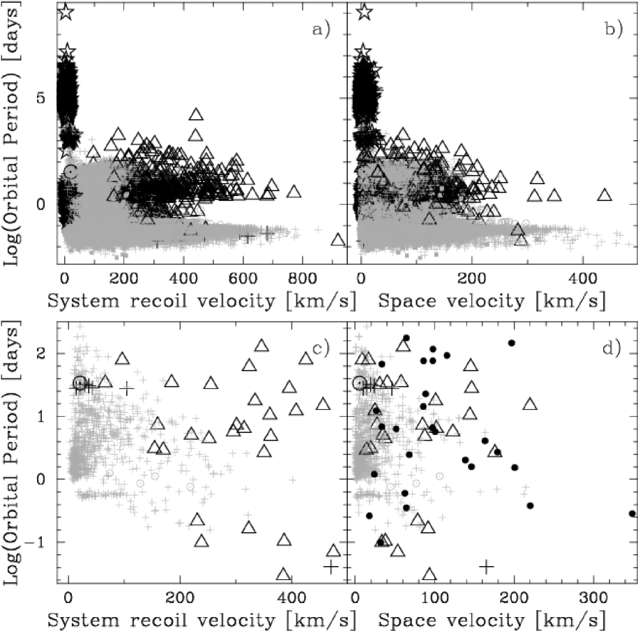
Figure 12: Parameter space of velocities (recoil and space) and orbital period for MSPs in Model C. The upper panels show all systems while the lower panels are restricted to include only pulsars with $B\geq 6\times 10^{7}~{}$G. The recoil velocities are with respect to the pre-NS binary CofM. The space velocities are with respect to the local standard of rest velocity (of $\sim 220~{}$km s^-1: Dehnen & Binney 1998). Identified are MSPs with MS star ($\odot$ symbols), giant star (solid squares), WD (plusses), NS (triangles) and BH (stars) companions. The large darker points represent those systems with eccentricities greater than $0.1$. The filled circles within panel d) represent the $28$ MSPs with observed transverse velocities and orbital periods taken from the ATNF Pulsar Catalogue.

We now examine the MSP population in velocity and orbital period parameter space. In terms of velocity we consider both the recoil velocity and the space velocity of the binary systems. The recoil velocity is defined as the change in velocity of the binary centre-of-mass owing to the SN explosion that created the NS (that went on to become the MSP). The space velocity is the velocity of the binary within the Galaxy at the time when the Galactic age is $10\,$Gyr. In calculating the final space velocities the solar motion around the Galactic centre is accounted for by removing the local standard of rest (LSR) velocity of $\sim 220~{}$km s^-1 (Dehnen & Binney 1998). The orbital period is taken as the final orbital period at a Galactic age of $10\,$Gyr. In a similar vein to Section 4.4.1 we examine the parameter space when considering all pulsars and then examine it again after limiting the sample population to MSPs that have $B\geq 6\times 10^{7}~{}$G. The results are shown in Figure 12.

The recoil velocities for all MSP binaries are shown in Figure 12a). The first item to note is the MSP-BH systems which all have low recoil velocities but cover a large range of final orbital periods. Such a distribution is not surprising given our detailed analysis of such systems in Section 4.4.2. Also not surprising is the rather large recoil velocity range of double-NS systems. The typical total recoil velocity incident on such systems is greater than $200~{}$km s^-1. We can also see from Figure 12a) that these systems are likely to be eccentric rather than circular. For MSP-NS systems that receive large recoil velocities ($>450~{}$km s^-1) there appears to be a lower limit to the possible final orbital period. The initial orbital period of these systems is very important in determining the evolution outcomes and the appearance of the final parameter space (Tauris & Bailes 1996). Also, in a related manner and as discussed for MSP-BH systems in Section 4.4.2, the onset of mass transfer and the details of the common-envelope phase are crucial factors. What we find is that a significant proportion of the double-NS population end up with extremely small periods (and a range of eccentricities) and coalesce rapidly (within a few Myr after double-NS formation) similar to that found by Belczynski, Bulik & Rudak (2002). This leads to the orbital period gap observed in Figure 12a). We leave further discussion on these systems for future work (Kiel, Hurley & Bailes, submitted). Turning to the MSP-WD systems we see that these typically receive rather low recoil velocities with the average value being less than $100~{}$km s^-1 (much less than $\sqrt{2}V_{\sigma}$) and in accordance to previous population synthesis results of Ramachandran & Bhattacharya (1997), Phinney & Kulkarni (1994), Lyne et al. (1998) and Sun & Han (2004). We also see that a similar but opposite trend occurs for MSP-WDs as did for the MSP-NSs in that for large recoil velocity values there appears to be an upper limit to the possible final orbital period. Again this is related to the orbital evolution and in particular whether a system enters common-envelope evolution (and survives without coalescence) or not.

Figure 12c) shows the recoil velocity and final orbital period parameter space for the magnetic-field limited MSP population. We see that the population has been significantly thinned out. In particular the entire MSP-BH population has been removed as have the low-period MSP-WD systems. It is also possible to compare our findings to the results of Tauris & Bailes (1996: see their Figure 2c) who followed the formation of MSPs using stellar and binary evolution algorithms that were quite advanced for their time. Compared to Tauris & Bailes (1996) we find less systems with orbital periods greater than a day. However, for the MSP-WD population we observe a similar trend of orbital period to recoil velocity: the smaller the orbital period the greater the range in possible recoil velocity of the system.

In Figure 12b) we look at the final space velocities and orbital periods for all MSP binaries. There is much similarity between the velocities given to each system (their recoil velocities) and their LSR Galactic motion. The form of this parameter space is therefore governed by the same evolutionary phases that dictated the appearance of Figure 12a). In Figure 12d) we show the space velocity-orbital period parameter space distribution of MSPs with $B\geq 6\times 10^{7}~{}$G. Included for comparison are pulsar proper motion observations which, convolved with distance estimates, give rise to observed transverse velocities. From the ATNF pulsar catalogue (Manchester, Hobbs, Teoh & Hobbs 2005) there are at present $28$ Galactic disk pulsars with spin periods less than $0.02~{}$s that have measured orbital periods and estimated transverse velocities. Although we do not directly compare total model space velocities to observed pulsar proper motions, useful information can still be gleaned from simple comparisons between the two noting that the transverse velocities are a lower limit to the true space motion (although measurement errors not included within Figure 12, especially in distance calculations, cloud this picture slightly). Firstly, once accounting for the LSR, we can see that many of the model MSP systems travel with speeds within the typical stellar velocity range of approximately $\pm 16~{}$km s^-1 (as given by Dehnen & Binney 1998). However, there appears to be an overabundance of model MSP binaries at low velocities. The model also fails to produce enough of the fast moving MSPs with large orbital periods. One reason for this may be the $V_{\sigma}=190~{}$km s^-1 assumed in Model C which is lower than the value suggested from observations ($V_{\sigma}=265~{}$km s^-1: Hobbs et al. 2005). On the other hand, Figure 12d) shows a large range of space velocities for MSP-NS systems. Perhaps surprisingly some of these systems even have velocities close to the LSR, although not so surprising according to Dewi, Podsiadlowski & Pols (2005) who suggest that DNSs receive small kicks. This is of particular interest for understanding the nature of the double pulsar J0737-3039 (Burgay et al. 2003) which is observed to have a transverse velocity of $30~{}$km s^-1 or less (Kramer et al. 2006). Considering that the system will have experienced two supernova events this has been taken as evidence for little or no velocity kicks within this system. However, Kalogera et al. (2007) have described models which show that kick velocities of $100~{}$km s^-1 or more are still possible. Our results agree with this in that it is not necessary to make any unusual assumptions regarding kicks in binary systems to explain the observed velocities of systems such as J0737-3039 (Deller, Bailes & Tingay 2009).

4.4.4 Effects of the assumed initial scale height

Up until now we have set a maximum of $|z_{\rm maxi}|=75~{}$pc to the initial birth height distribution of binaries, effectively modelling a thin disk. We now examine the effect this has on the scale height calculations by extending it to $|z_{\rm maxi}|=150~{}$pc in Model C${}^{{}^{\prime}}$. The results are compared to Model C in Table 4. We find that there is no significant change in the calculated scale heights. This agrees with previous works, such as Paczynski (1990) or Sun & Han (2004), who have suggested that for such kinematically active systems as pulsars the initial height above the plane does not greatly affect the outcome.

4.4.5 Effects of the assumed Galactic age

The age of the Galaxy is an important assumption, especially when populations of systems with large differences in life times are modelled together. To address this we have Model C${}^{{}^{\prime\prime}}$ which assumes the Galactic age is $15~{}$Gyr rather than $10~{}$Gyr for Model C. It is the isolated MSPs and MSP-NSs whose scale heights change the most appreciably in this new model compared to Model C. This is primarily owing to low number statistics (see Figure 8 for the relative numbers of the populations). Otherwise it does not appear that the increase in Galaxy age has a significant effect on the kinematics of the MSPs.

4.4.6 Sufficient model resolution?

Finally, to test whether our previous models have a fine enough resolution in the initial parameter space to faithfully represent the entire Galactic pulsar population we have extended Model C to include $10^{9}$ binary systems (a factor of $100$ increase). The only systems for which the scale height changed noticeably was the MSP-NS systems, which are relatively rare and kinematically energetic systems. In all other respects it appears that the results for $10^{7}$ systems scale reliably to larger populations. We note here that modelling $10^{9}$ binary systems is equivalent to modelling $\sim 10\%$ the mass of the Galaxy, assuming binary systems are of interest. To run a model of this size takes roughly $4500$ CPU hours and even when farming the model out to $100$ processors (on the Swinburne supercomputer) it takes almost $2~{}$days to complete. Thus it is obviously an advantage when examining a variety of evolutionary assumptions one model at a time to be able to represent the Galaxy faithfully with fewer systems.

5 Discussion

Using our newly developed binkin module for integrating the positions of stars and binaries within the Galaxy we have worked through a series of models in order to understand how various options available in the module affect the outcomes. This has allowed us to develop a favoured model – our Model C. In doing this we have used pulsar populations as our yardstick, computing scale heights, radial and velocity distributions, and orbital characteristics (in the case of binary systems) with limited comparison to observations. What we have done is to make predictions in all these areas about the particulars of the Galactic pulsar population, assuming that all pulsar systems can be observed. Of course this is not the case in reality and our model results cannot truly be confronted by observations until we include selection effects in our modelling. This will be completed when we add our next and final module binsfx to our population synthesis code. As such we leave a discussion of the necessary selection effects that need to be considered and their treatment to an upcoming paper focussed on the binsfx module (Kiel, Bailes & Hurley, in preparation). This paper will include features such as the predicted pulsar $P$-$\dot{P}$ diagram for distinct regions in the Galaxy (following on from our investigation of this diagram in Paper I in terms of binary evolution parameters). Below we discuss future additions to the binpop and binkin modules in relation to pulsar evolution as well as caveats to our current findings.

5.1 Accretion induced collapse formation of neutron stars

Further analysis of our MSP populations shows that some of the NSs which go on to become MSPs in our models are formed from the accretion induced collapse (AIC) of WDs (Canal & Schatzman 1976; Nomoto & Kondo 1991). In the scenario of Nomoto & Kondo (1991) an O-Ne-Mg WD accretes enough material to reach the Chandrasekhar mass, the maximum mass possible for a WD to support itself, and collapses to form a NS. To date we have allowed NSs formed in this way to receive velocity kicks in the same manner as for NSs formed in core-collapse SNe. Generally, if the binary system remains bound an AIC NS will continue to accrete material after the SN, a SN which induced an eccentricity into the orbit. This formation pathway produces a substantial number of MSP-WD and MSP-MS systems with eccentricities greater than $0.1$, that reside within the Galaxy. These systems highlight the importance of a correct mass-transfer treatment for eccentric binaries (see Paper I and Bonacic-Marinovic, Glebbeek & Pols 2008). This is something which is not currently accounted for in our models (we make use of equations which assume the orbit is circular: see HTP02) and it most likely will affect the production and visibility of these systems. Of course, if the AIC systems were not given any velocity kick, (as has been modelled previously: HTP02), or a much lighter kick (as latest models suggest: Dessart et al. 2006), then not only would there be many more AIC MSP systems but they would all have a greater possibility of residing in our Galactic target area and the population scale height would be lowered. They would also typically have smaller eccentricities.

Although we do not deal directly with low-mass X-ray binaries within this work it is possible for us to compare the observed scale heights of such systems – which suffer from less selection effects than pulsar observations – with our model MSP-MS scale height calculations. This is assuming that low-mass X-ray binaries are the progenitors of MSP-MS systems. Grimm, Gilfanov & Sunyaev (2002) found that Galactic field low-mass X-ray binaries have a scale height of $\sim 0.410~{}$kpc. Interestingly enough, as shown in Table 4, our models over estimate this by almost a factor of two. Such an outcome may be another implication that AIC NSs receive less momentum at birth than standard NSs formed from core-collapse SNe. However, it is not clear that MSPs that result from AIC NSs can be linked to an observable low-mass X-ray binaries phase (Hurley, Ferrario, Wickramasinghe, Tout & Kiel, in prep).

5.2 Electron capture supernovae

Another evolutionary scenario related to NS formation and velocity kicks is core-collapse electron capture SNe. This was discussed and modelled in Paper I and has also been accounted for in other population synthesis works (e.g. Ivanova et al. 2008). Briefly, core collapse electron capture SNe are thought to arise when electrons are captured onto Mg atoms, depleting the electron force in an O-Ne-Mg stellar core of sufficient mass ($1.4-2.5~{}M_{\odot}$: Nomoto 1984) which is produced by initial progenitor masses in the range of $8-12~{}M_{\odot}$ (although this mass range is model dependent: Podsiadlowski et al. 2004). The likelihood that a star born within the $8-12~{}M_{\odot}$ limit will evolve to have an O-Ne-Mg core mass between $1.4-2.5~{}M_{\odot}$ increases if the progenitor is able to interact with a companion and lose its outer hydrogen envelope, rather than evolve in an isolated environment (Podsaidlowski et al. 2004). Therefore, binary population synthesis is ideal for examining the likelihood and outcomes of such events. The resultant electron capture SN energy yield is low, sufficient to cause the explosion but not enough to impart any large velocity to the proto-NS (Kitaura, Janka & Hillebrandt 2006). Paper I found that the final MSP spin period and spin period derivative parameter space was altered when electron capture SNe were included. Less pulsar binary systems were disrupted, owing to the small momentum imparted during the SN, causing more MSPs to be produced. It is also reasonable to expect that including electron capture SNe in the binkin models, with SN kicks drawn from a distinct distribution with a smaller velocity dispersion than for standard NSs, will lead to a reduction in the pulsar scale heights. This is a feature that will be fully explored in future models so that the impact of the electron capture SNe process on binary evolution outcomes and the resultant Galactic kinematics of pulsar populations can be quantified.

5.3 MSP-BH systems

In our models we have assumed no SN velocity kick is given to BHs and have found that MSP-BH systems reside close to the Galactic plane. If BHs were instead to receive a SN kick selected from the same distribution as NSs then it is clear that the scale heights of populations including BHs would increase (Voss & Tauris 2003). However, it is not so obvious that the scale heights would be similar to that of the equivalent NS populations (Pfahl et al. 2005). In particular, MSP-BH systems (and their progenitors) will be heavier on average than MSP-NS systems (and their progenitors) and the more massive systems will require a greater momentum to reach the same velocities as less massive systems. As such MSP-BHs for example, could still have a significant difference in their resultant scale height to that of MSP-NSs even when both populations receive kicks from the same distribution. We would also expect the number of BH binary systems to decrease. Most likely it would be the MSP-BH systems with a large orbital periods prior to BH formation (systems with initial orbital periods greater than $\sim 100~{}$days) which would be depleted. It is these systems that are not produced in the models of Pfahl et al. (2005) who assume SN kicks occur on nascent BHs. However, we must bear in mind that the final BH masses are calculated assuming that material ejected in the SN falls back on to the BH. There is less mass-loss associated with BH formation than for NSs and this means supernova induced binary disruption is less likely during BH formation (in the case of equivalent kick velocities).

We note that when discussing the MSP-BH population (or any of our model MSPs) we are defining a rapidly rotating NS to be an MSP based solely on its spin period. If instead we also include consideration of the magnetic field strength of these NSs then the nomenclature may be misleading, especially if we are interested in observable MSPs. It turns out that all of the NSs in our model MSP-BH systems have magnetic fields residing on, or very close to, the assumed bottom magnetic field limit of $6\times 10^{7}~{}$G (Paper I; Zhang & Kojima 2006). Previously (Paper I, Figure 9 and Figure 12), we have assumed that any NS with a magnetic field less than this limit cannot accelerate the electrons in its atmosphere to produce the observed pulsar beam and as such is not observable as a pulsar. Therefore, if our assumptions regarding accretion on to NSs and how this translates to magnetic field decay are correct then we have a lot of trouble producing observable MSP-BHs. Future observations of such systems will help greatly in constraining our evolutionary assumptions.

5.4 Initial distributions

In our models we have assumed a maximum birth height off the plane, $|z_{\rm maxi}|$, of either 75 or $150\,$pc. Consistent with Paczynski (1990) and Sun & Han (2004) no significant variations of the MSP population scale heights were found when varying this parameter. This suggests that the results are robust to changes in $|z_{\rm maxi}|$ as long as a sensible choice is made. The majority of OB star formation has been shown by de Wit, Testi, Palla & Zinnecker (2005) to occur within $|z|\sim 200~{}$pc of the Galactic plane so choices within this range, such as for our models, would seem reasonable. In the future it will be interesting to probe the effects of assuming a radial dependence in $|z_{\rm maxi}|$ on the final pulsar population distributions. This may even be tied in with examining the effect of assuming bursts of star formation throughout the age of the Galaxy and accounting for Galactic arms when initiating the birth positions. This final point has previously been suggested as an important feature to incorporate into population synthesis models (Faucher-Giguere & Kaspi, 2007).

We found that the Yusifov & Kucuk (2004) initial radial pulsar birth distribution gave the best fit of our models to observations. This distribution was based on observations of HII regions within the Galaxy. However, it failed to reproduce the peak of the observable radial distribution – which the Paczynski (1990) initial radial distribution succeeded in reproducing. Yusifov & Kucuk (2004) recognised that their relation is approximate and suggested that a detailed analysis between models and observations of pulsar velocities and Population I stellar positions was required to develop a more realistic distribution. We are in a position to do this and as a result can suggest that the initial pulsar birth distribution of Yusifov & Kucuk (2004) perhaps be shifted towards smaller Galactic radii to peak at the inner HII peak ($\sim 4.0-4.5~{}$kpc) depicted in Figure 3 of Paladini, Davis & DeZotti (2004).

5.5 Galactic model potentials

Even though our favoured model (Model C) utilises the Pac90 form of the Galactic gravitational potential we are in no way able to distinguish between this and the KG89 model as a more suitable representation of the Galactic potential. Both give similar pulsar population scale height results which is not surprising given their similarities as shown in Figure 4. The form of the Xue08 potential is clearly distinct from the other two models, especially within the inner $1\,$kpc of the Galaxy (where Xue08 employ an extrapolation of their measurements), and leads to markedly increased scale heights. On this basis we do not favour use of the Xue08 potential. However, we are not currently in a position to make strong conclusions in this area, especially when many previous pulsar, NS and X-ray binary population synthesis works (such as Paczynski 1990, Lorimer et al. 1993, Belczynski, Bulik & Rudak 2002, Sun & Han 2004 and Zuo, Li & Liu 2008) have used different Galactic gravitational potentials and their results compare well to observations. We note that Sun & Han (2004) comment that it is unclear whether the Milky Way has a peak in the gravitational potential at small Galactic radii (as present in the Pac90 and KG89 models).

A possibility in the future is to extend the Galactic gravitational potential analysis to consider Modified Newtonian Dynamics (MoND). Such an approach has already been taken by Wu et al. (2008), who compare MoND with cold dark matter models, and Zuo, Li & Liu (2008) who make use of MoND potentials to conduct population synthesis of X-ray binaries.

5.6 Close double compact systems and gamma ray bursts

In this work we have focussed on pulsars and looked in detail at MSP systems. However, the models can also be extended to explore the formation of close double compact systems (NS-NS, BH-BH and NS-BH systems) in detail. The kinematics of these systems is of interest because of their link to gamma-ray bursts and, in particular, recent observations of the distances at which gamma-ray bursts appear to occur from their (assumed) host galaxy (Bloom, Kulkarni & Djorgovski 2002). Our combined binpop and binkin modules can provide model estimates for the projected distances from their host galaxy at which double compact systems coalesce and document the kinematic evolution of these systems in general. This will be the focus of a companion paper (Kiel, Hurley & Bailes, submitted).

6 Summary

We have examined in depth the Galactic dynamics and population characteristics (owing to stellar, binary and kinematic evolution) of pulsars. Our main findings, reconfirming and updating many areas of pulsar evolutionary physics, can be summarised as follows (noting that overlap with previous work is detailed in Section 4):

• When using a peaked radial distribution for the birth locations of binaries, the population of pulsars that arises from these binaries also follows a peaked distribution where the location of the peak moves inwards in radius by as much as $0.5\,$kpc as the population evolves. Also, compared to the birth distribution, the initial shape is preserved inward of the peak but the distribution becomes more extended in the outer regions.

• Starting with a uniform initial distribution of binaries cannot produce a final pulsar distribution that is peaked away from the centre of the Galaxy and therefore does not compare well to observations of pulsar locations which indicate a deficit of pulsars towards the Galactic centre.

• The form of the Galactic potential does not produce significant differences in the final radial distribution of pulsars but can lead to noticeable differences in the calculated scale heights of pulsars.

• As the pulsar population ages the peak of its velocity distribution moves to lower velocities. The velocity dispersion of this distribution (assuming a Maxwellian) almost halves over a period of $10\,$Gyr. The shape of the velocity distribution is significantly affected by the the inclusion of binary evolution – this produces a more sharply peaked distribution.

• Similar to observations we find that the majority of standard pulsars are isolated and that these dominate the statistics of the pulsar scale height calculations.

• Isolated pulsars have a greater scale height than binary pulsars except in cases where large velocity kicks are applied to the population resulting in many isolated pulsars being lost from the Galaxy and hence from the scale height calculations.

• Isolated MSPs have greater scale heights than binary MSPs (by as much as a factor of two) however, limiting the region of the Galaxy considered (in terms of height off the plane) does reduce the difference in these scale heights and brings them more in line with what observations suggest.

• We find that 99% of MSPs are in binary systems when we only consider SN disruption as a pathway for creating isolated MSPs. This does not agree with the observed MSP population. If we include a simple ablation model we find instead that 64% of MSPs are in binaries which adequately matches the observed mix. Furthermore, accounting for ablation gives similar scale heights for isolated and binary MSPs.

• MSP systems with NS companions can receive large recoil velocities. There is a large scatter in the resulting peculiar motions of MSP-NS binaries and it is possible for such systems to found with low peculiar motion.

• The scale heights of the MSP-MS and MSP-WD binary populations are very similar and follow similar radial distributions. These scale heights are larger than that of the observed low-mass X-ray binary population in the Galaxy (often thought to be the precursors of MSP-MS binaries). However, many of the model MSPs in binary systems are formed from the accretion-induced collapse of a WD which, if given smaller kicks than for standard NSs at birth, would reduce the model scale heights.

• MSPs with WD companions are the most common of the binary MSPs. This is followed by MSP-MS, MSP-BH and MSP-NS binaries, respectively.

• Restricting the model MSP population to only include MSPs with magnetic fields greater than $6\times 10^{7}\,$Gauss drastically reduces the number of systems and changes the way that the population is distributed. This suggests that the underlying pulsar distribution of the Galaxy may differ greatly from the observed sample.

One future goal of pulsar astronomy is the detection of a pulsar orbiting a black hole, and in terms of placing constraints upon general relativity a millisecond pulsar in a close orbit around a black hole would be an especially exciting observation. We find three distinct evolutionary pathways which result in the formation of MSP-BH systems. These pathways produce three distinct MSP-BH populations in terms of orbital period: those with periods of $10\,$day or less, those with periods of about $1\,000\,$days, and those with periods of $10\,000\,$day or greater. The short and long period populations are the most numerous and only the short-period systems are found further than $1\,$kpc from the Galactic plane. We find that owing to the amount of material accreted by the MSPs in our model MSP-BH binaries that the magnetic field decays below $6\times 10^{7}\,$Gauss. This possibly suggests that we are overestimating the rate of accretion-induced magnetic field decay in our evolution model – the observation of a MSP-BH binary would confirm this possibility.

We emphasise to the reader that we are not presenting any of the models in this paper as a definitive representation of the true Galactic pulsar population. The uncertainty involved in the many parameters contained within binpop and binkin does not allow this. Moreover, because we do not consider selection effects in our model Galaxy we cannot at this stage make definitive comparisons to observations as the possibility exists that the observed population may be biased in some manner. Lommen et al. (2007) suggest that observations of MSPs may preferentially detect binary MSPs because the isolated MSPs may be less luminous than their binary cousins. The intrinsic luminosity of pulsars is not something examined in this body of work. However, it will be discussed in detail in future work where selection effects are calculated within our upcoming binsfx module (Kiel, Bailes & Hurley, in prep). Supplementing our current pulsar population synthesis with selection effects will allow additional evaluation of the evolutionary codes and their scientific outcomes. It will also allow us to guide further surveys by selecting regions of the sky best suited for the specific pulsar survey and/or telescope of interest. Therefore binsfx will provide a powerful tool with which to constrain the theory and modelling of stellar, binary and Galactic kinematic evolution. Further constraints could be placed on binary evolution if population synthesis studies are extended to include additianal stellar populations and their appropriate selection effects. For now, however, we are well on our way to producing a comprehensive treatment of pulsar population physics.

Appendix A

The time taken for a star to be ablated by a MSP can be approximated by taking the irradiated luminosity onto the companion, which is of order

$$L\sim\frac{\Delta E}{\Delta t}\sim 4.4\times 10^{32}\rm{ergs^{-1}},$$ (35)

(Tavani, 1992) and equating $\Delta E$ with the change in binding energy of the companion,

$$E_{bind}=\frac{GM_{\star}^{2}}{R_{\star}},$$ (36)

Solving $\Delta t$ for the threshold mass of a $0.02~{}M_{\odot}$ star (Tavani 1992) gives $\Delta t=5.5~{}$Myr, while for a $0.01~{}M_{\odot}$ star $\Delta t=2.7~{}$Myr.

References

- Abell & Margon (1979) Abell G.O., Margon B., 1979, Nature, 279, 701
- Arzoumanian, Chernoff & Cordes (2002) Arzoumanian Z., Chernoff D.F., Cordes J.M., 2002, ApJ, 568, 289
- Backer et al. (1982) Backer D.C., Kulkarni S.R., Heiles C., Davis M.M., Goss W.M., 1982, Nature, 300, 615
- Bailes (1989) Bailes M., 1989, ApJ, 324, 917
- Belczynski, Bulik & Rudak (2002) Belczynski K., Bulik T., Rudak B., 2002, ApJ, 571, 394
- Belczynski, Kalogera & Bulik (2002) Belczynski K., Kalogera V., Bulik T., 2002, ApJ, 572, 407
- Belczynski et al. (2008) Belczynski K., Kalogera V., Rasio F.A., Taam R.E., Zezas A., Bulik T., Maccarone T.J., Ivanova N., 2008, ApJS, 174, 223
- Bhattacharya & van den Heuvel (1991) Bhattacharya D., van den Heuvel E.P.J., 1991, PhR, 203, 1
- Binney (1982) Binney J., 1982, MNRAS, 201, 1
- Bisnovatyi-Kogan & Komberg (1974) Bisnovatyi-Kogan G.S., Komberg B.V., 1974, SvA, 18, 217
- Bloom, Kulkarni & Djorgovski (2002) Bloom J.S., Kulkarni S.R., Djorgovski S.G., 2002, ApJ, 123, 1111
- Bogomazov, Lipunov & Tutukov (2008) Bogomazov A.I., Lipunov V.M., Tutukov A.V., 2008, ARep, 52, 463
- Bonačić Marinović, Glebbeek & Pols (2008) Bonačić Marinović A.A., Glebbeek E., Pols O.R., astro-ph/0710.4859, accepted by A&A
- Burgay et al. (2003) Burgay M., et al., 2003, Nature, 426, 531
- Canal & Schatzman (1976) Canal R., Schatzman E., 1976, A&A, 46, 229
- Carlberg & Innanen (1987) Carlberg R.G., Innanen K.A., 1987, ApJ, 94, 666
- Chen & Ruderman (1993) Chen K., Ruderman M., 1993, ApJ, 402, 264
- Combi, Albacete-Colombo & Marti (2008) Combi J.A., Albacete-Colombo J.F., Marti J., 2008, A&A, 477, 125
- Cordes Romani & Lundgren (1993) Cordes J.M., Romani R.W., Lundgren S.C., 1993, Nature, 362, 133
- Cordes & Lazio (2002) Cordes J.M., Lazio T.J.W., 2002, astro-ph/020756
- Cordes et al. (2006) Cordes J.M., et al., 2006, ApJ, 637, 446
- Chen & Ruderman (1993) Chen K., Ruderman M., 1993, ApJ, 408, 179
- Davis et al. (2008) Davis D.S., Richer H.B., King I.R., Anderson J., Coffey J., Fahlman G.G., Hurley J., Kalirai J.S., 2008, MNRAS, 383, 20
- Dehnen & Binney (1998) Dehnen W., Binney J., 1998, MNRAS, 294, 429
- Deller, Bailes & Tingay (2009) Deller A.T., Bailes M., Tingay S.J., 2009, accepted in Science, arXiv:0902.0996
- Dessart et al. (2006) Dessart L., Burrows A., Ott C.D., Livne E., Toon S.-C., Langer N., 2006, ApJ, 644, 1063
- Dewey & Cordes (1987) Dewey R.J., Cordes J.M., 1987, ApJ, 321, 780
- Dewi, Podsiadlowski & Pols (2005) Dewi J.D.M., Podsiadlowski Ph., Pols O.R., 2005, MNRAS, 363, 71
- de Wit, Testi, Palla & Zinnecker (2005) de Wit W.J., Testi L., Palla F., Zinnecker H., 2005, A&A, 437, 247
- Eichler & Livinson (1988) Eichler D., Livinson A., 1988, ApJ, 355, 67
- Faucher-Giguere & Kaspi (2006) Faucher-Giguere C., Kaspi V.M., 2006, ApJ, 643, 332
- Fellhauer et al. (2003) Fellhauer M., Lin D.N.C., Bolte M., Aarseth S.J., Williams K.A., 2003, ApJ, 595, 53
- Ferrario & Wickramasinghe (2007) Ferrario L., Wickramasinghe D., 2007, MNRAS, 375, 1009
- Fryer & Kalogera (2001) Fryer C.L., Kalogera V., 2001, ApJ, 545, 548
- Freire, Ransom & Gupter (2007) Freire P.C.C., Ransom S.M., Gupter Y., 2007, ApJ, 662, 1177
- Galloway et al. (2008) Galloway D.K., Muno M.P., Hartman J.M., Psaltis D., Chakrabary D., 2008, ApJS accepted, astro-ph/0608259v2
- Goldreich & Julian (1969) Goldreich P., Julian W.H., 1969, ApJ, 157, 869
- Gott, Gunn & Ostriker (1970) Gott J.R., Gunn J.E., Ostriker J.P., 1970, ApJ, 160, L91
- Grimm, Gilfanov & Sunyaev (2002) Grimm H.J., Gilfanov M., Sunyaev R., 2002, A&A, 391, 923
- Gunn & Ostriker (1970) Gunn J.E., Ostriker J.P., 1970, ApJ, 160, 979
- Hansen & Phinney (1997) Hansen B.M.S., Phinney E.S., 1997, MNRAS, 291, 569
- Harding, Muslimov & Zhang (2002) Harding A.K., Muslimov A.G., Zhang B., 2002, ApJ, 576, 375
- Hernquist (1990) Hernquist L., 1990, ApJ, 356, 359
- Hewish et al. (1968) Hewish A., Bell S.J., Pilkington J.D., Scott P.F., Collins R.A., 1968, Nature, 217, 709
- Heyl (2007) Heyl J., 2007, MNRAS, 382, 915
- Hills (1983) Hills J.G., 1983, ApJ, 267, 322
- Hobbs et al. (2005) Hobbs G., Lorimer D.R., Lyne A.G., Kramer M., 2005, MNRAS, 360, 974
- Huang & Becker (2007) Huang H.H., Becker W., 2007, A&A, 463, 5
- Hulse & Taylor (1975) Hulse R.A., Taylor J.H., 1975, ApJ, 195, 51
- Hurley, Pols & tout (2000) Hurley J.R., Pols O.R., Tout C.A., 2000, MNRAS, 315, 543
- Hurley, Tout & Pols (2002) Hurley J.R., Tout C.A., Pols O.R., 2002, MNRAS, 329, 897 (HTP02)
- Iben, Tutukov & Yungelson (1995) Iben, I.J., Tutukov A.V., Yungelson L.R., 1995, ApJS, 100, 233
- Ivanova et al. (2008) Ivanova N., Heinke C.O., Rasio F.A., Belczynski K., Fregeau J.M., 2008, MNRAS, 386, 553
- Jonker & Nelemans (2004) Jonker P.G., Nelemans G., 2004, MNRAS, 354, 355
- Kalkarni & Narayan (1988) Kalkarni S.R., Narayan R., 1988, ApJ, 335, 755
- Kalogera (1996) Kalogera V., 1996, ApJ, 471, 352
- Kalogera (1998) Kalogera V., 1998, ApJ, 493, 368
- Kalogera et al. (2007) Kalogera V., Belczynski K., Kim C., O’Shaughnessy R., Willems B., 2007, Physics Reports, 442, 75
- Kaspi et al. (1996) Kaspi V.M., Bailes M., Manchester R.N., Stappers B.W., Bell J.F., 1996, Nature, 381, 984
- Kiel & Hurley (2006) Kiel P.D., Hurley J.R., 2006, MNRAS, 369, 1152
- Kiel, Hurley, Bailes & Murray (2008) Kiel P.D., Hurley J.R., Bailes M., Murray J.R., 2008, MNRAS, 388, 393 (Paper I)
- Kitaura, Janka & Hillebrandt (2006) Kitaura F.S., Janka H.-Th., Hillebrandt W., 2006, A&A, 450, 345
- Klebesadel, Strong & Olson (1973) Klebesadel R.W., Strong I.B., Olson R.A., 1973, ApJ, 182, 85
- Kramer (1998) Kramer M., 1998, ApJ, 509, 856
- Kramer et al. (2006) Kramer M., et al., 2006, Science, 314, 97
- Kuijken & Gilmore (1989) Kuijken K., Gilmore G., 1989, MNRAS, 239, 571
- Kulkarni & Narayan (1988) Kulkarni S.R., Narayan R., 1988, ApJ, 335, 755
- Landau & Lifshitz (1951) Landau L.D., Lifshitz E.M., 1951, The Classical Theory of Fields, 4th edn. Pergamon Press, Oxford
- Lee et al. (2008) Lee T.S., et al., 2008, AJ, 136, 2022
- Lipunov et al. (1994) Lipunov V.M., Postnov K.A., Prokhorov M.E., Osminkin E.Yu., 1994, ApJ, 423, 121
- Lipunov, Bogomazov & Abubekerov (2005) Lipunov V.M., Bogomazov A.I., Abubekerov M.K., 2005, MNRAS, 359, 1517
- Liu, van Paradijs & van den Heuvel (2007) Liu Q.Z., van Paradijs J., van den Heuvel E.P.J., 2007, A&A, 469, 807
- Lommen, et al. (2006) Lommen A.N., Kipphorn R.A., Nice D.J., Splaver E.M., Stairs I.H., Backer D.C., 2006, ApJ, 642, 1012
- Lorimer et al. (1993) Lorimer D.R., Bailes M., Dewey R.J., Harrison P.A., 1993, MNRAS, 263, 403
- Lorimer, Bailes & Harrison (1997) Lorimer D.R., Bailes M., Harrison P.A., 1997, MNRAS, 289, 592
- Lorimer (2005) Lorimer D.R., 2005, Living Rev. Relativity 8, URL (cited on 23/06/2008)
- Lorimer et al. (2006) Lorimer D.R., et al., 2006, MNRAS, 372, 777L
- Lorimer et al. (2007) Lorimer D.R., McLaughlin M.A., Champion D.J., Stairs I.H., 2007, MNRAS, 379, 282
- Lyne et al. (1998) Lyne A.G., et al., 1998, MNRAS, 295, 743L
- Lyne et al. (2004) Lyne et al. 2004, Science, 303, 1153L
- Lyne & Lorimer (1994) Lyne A.G., Lorimer D.R., 1994, Nature, 369, 127
- Manchester, Hobbs, Teoh & Hobbs (2005) Manchester R.N., Hobbs G.B., Teoh A., Hobbs M., 2005, ApJ, 129, 1993
- Margon et al. (1979) Margon B,. Ford H.C., Katz J.I., Kwitter K.B., Ulrich R.K., Stone R.P.S., Klemola A., 1979, ApJ, 230, 41
- McGlynn (1984) McGlynn T.A., 1984, ApJ, 281, 13
- Miyamoto & Nagai (1975) Miyamoto M., Nagai R., 1975, PASJ, 27, 533
- Narayan & Ostriker (1990) Narayan R., Ostriker J.P., 1990, ApJ, 352, 222
- Narayan, Piran & Shemi (1991) Narayan R., Piran T., Shemi A., 1991, ApJ, 379, 17
- Navarro, Frenk & White (1996) Navarro J.F., Frenk C.S., White S.D.M., 1996, ApJ, 462, 563
- Nomoto (1984) Nomoto K., 1984, ApJ, 277, 791
- Nomoto & Kondo (1991) Nomoto K., Kondo Y,. 1991, ApJ, 367, 19L
- O’Shaughnessy, Kim, Kalogera, Belczynski (2008) O’Shaughnessy R., Kim C., Kalogera V., Belczynski K., 2008, 672, 479
- Ostriker & Gunn (1969) Ostriker J.P., Gunn J.E., 1969, ApJ, 157, 1395
- Paczynski (1986) Paczynski B., 1986, ApJ, 308, 43
- Paczynski (1990) Paczynski B., 1990, ApJ, 348, 485
- Paladini, Davis & DeZotti (2004) Paladini R., Davies R.D., DeZotti G., 2004, MNRAS, 347, 237
- Plummer (1911) Plummer H.C., 1911, MNRAS, 71, 460
- Pfahl, Rappaport & Podsaidlowski (2003) Pfahl E., Rappaport S., Podsaidlowski P., 2003, ApJ, 597, 1036
- Pfahl, Rappaport & Podsaidlowski (2005) Pfahl E., Podsaidlowski P., Rappaport S., 2005, ApJ, 628, 343
- Phinney & Kulkarni (1994) Phinney E.S., Kulkarni S.R., 1994, Ann. Rev. Astron. Astrophys., 32, 591
- Podsiadlowski, Rappaport & Han (2003) Podsiadlowski P., Rappaport S., Han Z., 2003, MNRAS, 341, 385
- Podsaidlowski et al. (2004) Podsiadlowski P., Langer N., Poelarends A.J.T., Rapparport S., Heger A., Pfahl E., 2004, ApJ, 612, 1044
- Portegies Zwart & Yungelson (1998) Portegies Zwart S.F., Yungelson A., 1998, A&A, 372, 173
- Ramachandran & Bhattacharya (1997) Ramachandran R., Bhattacharya D., 1997, MNRAS, 288, 565
- Rantsiou, Kobayashi, Laguna & Rasio (2008) Rantsiou E., Kobayashi S., Laguna P., Rasio F.A., 2008, ApJ, 680, 1326
- Ruderman et al. (1988) Ruderman M., Shaham J., Tavani M., Eichler D., 1989, ApJ., 343, 292
- Schreier et al. (1972) Schreier E., Levinson R., Gursky H., Kellogg E., Tananbaum H., Giacconi R., 1972, ApJ, 172, 79
- Shklovskii (1970) Shklovskii I., 1970, Astron. Zh., 46, 715
- Spruit (1998) Spruit H.C., 1998, A&A, 333, 603
- Smith et al. (2007) Smith M.C., et al., 2007, 379, 755
- Stollman & van den Heuvel (1986) Stollman G.M., van den Heuvel E.P.J., 1986, 162, 87
- Sun & Han (2004) Sun X.H., Han J.L., 2004, MNRAS, 350, 232
- Tauris & Bailes (1996) Tauris T.M., Bailes M., 1996, A&A, 315, 432
- Tauris & Takens (1998) Tauris T.M., Takens R.J., 1998, A&A, 330, 1047 (T&T98)
- Tavani (1992) Tavani M., 1992, A&A, 261, 472
- Taylor & Manchester (1977) Taylor J.H., Manchester R.N., 1977, ApJ, 215, 885
- Toomre (1963) Toomre A, 1963, ApJ, 138, 385
- Valluri & Merritt (1998) Valluri M., Merritt D., 1998, A&A, 330, 1047
- van den Heuvel (1984) van den Heuvel E.P.J., 1984, A&A, 5, 209
- van Paradijs et al. (1988) van Paradijs J., Allington-Smith J., Callanan P., Hassall B.J.M., Charles P.A., 1988, Nature, 334, 684
- Wu et al. (2008) Wu X., Famaey B., Gentile G., Perets H., Zhao H.S., 2008, MNRAS, 386, 2199
- Xue et al. (2008) Xue X.-X., et al., 2008, ApJ, 684, 1143
- York et al. (2000) York D.G., et al., 2000, AJ, 120, 1579
- Yusifov & Kucuk (2004) Yusifov I., Kucuk I., 2004, A&A, 422, 545
- Zhang & Kojima (2006) Zhang C.M., Kojima Y., 2006, MNRAS, 366, 137
- Zuo, Li & Liu (2008) Zuo Z.-Y., Li X.-D., Liu X.-W., 2008, MNRAS, 387, 121