Confronting the damping of the baryon acoustic oscillations with observation

Abstract

We investigate the damping of the baryon acoustic oscillations in the matter power spectrum due to the quasinonlinear clustering and redshift-space distortions by confronting the models with the observations of the Sloan Digital Sky Survey luminous red galaxy sample. The chi-squared test suggests that the observed power spectrum is better matched by models with the damping of the baryon acoustic oscillations rather than the ones without the damping.

I Introduction

The baryon acoustic oscillations (BAO), the sound oscillations of the primeval baryon-photon fluid prior to the recombination epoch, left their signature in the matter power spectrum EH ; MWP . The BAO signature in the galaxy clustering has recently attracted remarkable attention as a powerful probe for exploring the nature of the dark energy component commonly believed to be responsible for the accelerated expansion of the Universe Eisenstein ; Hutsi ; PercivalI ; PercivalII ; Tegmark ; Yamamoto03 . The usefulness of the BAO to constrain the dark energy has been demonstrated PercivalIII ; Okumura ; HutsiII , and a lot of the BAO survey projects are in progress or planned sdss3 ; Bassett ; lsst ; ska ; Robberto . The BAO signature in the matter clustering plays a role of the standard ruler, because the characteristic scale of the BAO is well understood within the cosmological linear perturbation theory as long as the adiabatic initial density perturbation is assumed.

However, the comparison of the BAO signature with observation is rather complicated. The observed galaxy power spectrum is contaminated by the nonlinear evolution of the density perturbations, the redshift-space distortions and the clustering bias. This enables us to use the galaxy power spectrum for other supplementary tests, in addition to the test of the expansion history of the Universe for the equation of state of the dark energy. For example, the redshift-space distortions probe the linear growth rate of the density fluctuations Guzzo ; YSH ; PS . The growth rate is now recognized to be very important as the test of gravity on the cosmological scales.

In the paper Nomura , some of the authors of the present paper investigated how the quasinonlinear density perturbations affect the BAO signature. Especially, we focused on the damping of the BAO signature. The semianalytic investigation on the basis of the third-order perturbation theory demonstrated that the BAO damping is sensitive to the growth factor $D_{1}(z)$ and the amplitude of the matter power spectrum $\sigma_{8}$. Here $z$ is the redshift and the growth factor is normalized as $D_{1}(z)=a$ at $a\ll 1$, where $a$ is the scale factor normalized as $a=1$ at the present epoch. As a result, a measurement of the BAO damping might be useful as an additional consistency test by enabling one to probe the growth factor multiplied by the amplitude of the matter perturbation $D_{1}(z)\sigma_{8}$. In the present paper, we extend the previous work to include the redshift-space distortions, and confront the BAO damping with the observed SDSS LRG galaxy power spectrum. Throughout this paper, we use units in which the velocity of light equals 1, and adopt the Hubble parameter $H_{0}=100h{\rm km/s/Mpc}$ with $h=0.7$.

II Damping of the BAO

We start with reviewing the theoretical modeling of the BAO damping. The BAO signature is extracted from the matter power spectrum $P({k,\mu},z)$ at redshift $z$ in the following manner,

$$B({k,\mu},z)\equiv{P({k,\mu},z)\over{\widetilde{P}}({k,\mu},z)}-1,$$ (1)

where $\mu$ is the cosine of the angle between the line of sight direction and the wave number vector, and ${\widetilde{P}}({k,\mu},z)$ is the corresponding smooth spectrum without the BAO. As will be explained in detail below, we adopt the formalism developed by Matsubara Matsubara for theoretical modeling of $P({k,\mu},z)$. The corresponding smooth spectrum ${\widetilde{P}}({k,\mu},z)$ is computed in the same manner as $P({k,\mu},z)$ but with the no-wiggle transfer function in Ref. EH . As an alternative method, one can utilize the cubic spline fitting method to construct the smooth spectrum PercivalII ; Nishimichi , which we adopt in comparison with observations.

The modeling of the quasinonlinear power spectrum has been investigated by many authors, based on both the perturbation theory and numerical simulations. As a nonperturbative approach beyond the standard perturbation theory, Matsubara proposed a model of the quasinonlinear matter power spectrum using the technique of resuming infinite series of higher order perturbations on the basis of the Lagrangian perturbation theory (LPT) Matsubara . One of the advantages of using the LPT framework is the ability to calculate the quasinonlinear matter power spectrum in redshift space, which can be obtained by

$$P_{\rm LPT}^{({\rm s})}({k,\mu},z)=e^{-\alpha(\mu,z)D_{1}^{2}(z)g(k)}\left[D_{1}^{2}(z)P_{{\rm lin}}^{(s)}({k,\mu})+D_{1}^{4}(z)P_{2}^{(s)}({k,\mu})+\alpha(\mu,z)D_{1}^{4}(z)g(k)P_{{\rm lin}}^{(s)}({k,\mu})\right],$$ (2)

where

$$g(k)={k^{2}\over 6\pi^{2}}\int_{0}^{\infty}dqP_{{\rm lin}}^{({\rm r})}(q),$$ (3)

$$P_{{\rm lin}}^{(s)}({k,\mu})=\left(1+f\mu^{2}\right)^{2}P_{{\rm lin}}^{({\rm r})}(k),$$ (4)

$P_{{\rm lin}}^{({\rm r})}(k)$ is the linear matter power spectrum at the present epoch, $f=d\ln D_{1}/d\ln a$, and $\alpha(\mu,z)=1+f(f+2)\mu^{2}$. Also, $P_{2}^{(s)}(k)$ is expressed as

$$P_{2}^{(s)}({k,\mu}) = P_{22}^{({\rm s})}({k,\mu})+P_{13}^{({\rm s})}({k,\mu}),$$ (5)

where

$$P_{22}^{({\rm s})}({k,\mu})=\sum_{n,m}\mu^{2n}f^{m}{k^{3}\over 4\pi^{2}}\int_{0}^{\infty}drP_{{\rm lin}}^{({\rm r})}(kr)\int_{-1}^{1}dxP_{{\rm lin}}^{({\rm r})}[k(1+r^{2}-2rx)^{1/2}]{A_{nm}(r,x)\over(1+r^{2}-2rx)^{2}},$$ (6)

$$P_{13}^{({\rm s})}({k,\mu})=(1+f\mu^{2})P_{{\rm lin}}^{({\rm r})}(k)\sum_{n,m}\mu^{2n}f^{m}{k^{3}\over 4\pi^{2}}\int_{0}^{\infty}drP_{{\rm lin}}^{({\rm r})}(kr)B_{nm}(r),$$ (7)

and $A_{nm}(r,x)$ and $B_{nm}(r)$ are given in Appendix B of Ref. Matsubara . We take $P_{\rm LPT}^{({\rm s})}({k,\mu},z)$ as $P({k,\mu},z)$ in Eq. (1).

Figure 1: The BAO signature according to the linear theory and the LPT formalism. Except for the lower right panel, the dotted curve is the linear theory, the solid curve is the LPT formula, and the dashed curve uses the approximate formula Eq. (10), for $\mu=0,~{}0.5$, and $1$, respectively. The lower right panel summarizes the $\mu$-dependence, obtained with Eq. (8). The (quasinonlinear) redshift-space distortion causes more damping of the BAO signature. Here the redshift is $z=1$, and the cosmological parameters are $h=0.7$, $\Omega_{m}=0.27$, $\Omega_{b}=0.046$, $n_{s}=0.96$ and $\sigma_{8}=0.82$

.

Figure 2: Relative error $|\delta B/B|=|B_{\rm ex}-B_{\rm ap}|/|B_{\rm ex}|$ at the wave numbers P1, P2, P3, T1, T2 and T3, which correspond to the peaks and troughs defined in Fig. 1, as a function of the redshift. Except for the right lower panel, the cases $\mu=0,~{}0.5$, and $1$ are shown, respectively. The right lower panel shows the result for the angular averaged power spectrum $|\delta B/B|=|B^{\rm ave}_{\rm ex}-B^{\rm ave}_{\rm ap}|/|B^{\rm ave}_{\rm ex}|$.

Figure 1 shows the BAO signature. Except for the right lower panel, the dotted curve is the linear theory, while the solid curve is the result from the LPT formula at redshift $z=1$ for $\mu=0,~{}0.5$, and $1$, respectively, which is explicitly given by

$$B_{\rm ex}({k,\mu},z)={P_{\rm LPT}^{({\rm s})}({k,\mu},z)\over{\widetilde{P}}_{\rm LPT}^{({\rm s})}({k,\mu},z)}-1.$$ (8)

The right lower panel summarizes the $\mu$ dependence, which is given by Eq. (8). Note that the case $\mu=0$ is equivalent to the LPT formula in real space. The amplitude of the BAO signature is degraded compared with the linear perturbation theory. Thus the quasinonlinear clustering and the redshift-space distortions decrease the amplitude of the BAO.

Let us introduce the correction function of the BAO damping $W({k,\mu},z)$ by

$$B_{\rm ap}({k,\mu},z)=\left[1-W({k,\mu},z)\right]B_{{\rm lin}}(k),$$ (9)

where $B_{{\rm lin}}(k)$ is the BAO signature in linear theory. In the previous paper Nomura , which was restricted to real space, it was demonstrated that the correction factor can be written in a rather simple form. One of the main results of the present paper is that a similar simple formula can be derived in redshift-space. After some computation similar to the one in Nomura , we found that the leading factor of the correction function can be approximately written as

$$W({k,\mu},z)={D_{1}^{2}(z)\over 1+\alpha(\mu,z)D_{1}^{2}(z)\tilde{g}(k)}{{\widetilde{P}}_{22}^{({\rm s})}({k,\mu})\over{\widetilde{P}}_{{\rm lin}}^{({\rm s})}({k,\mu})},$$ (10)

where ${\widetilde{P}}_{22}^{({\rm s})}({k,\mu})$ and ${\widetilde{P}}_{{\rm lin}}^{({\rm s})}({k,\mu})$ are defined as $P_{22}^{({\rm s})}({k,\mu})$ and $P_{{\rm lin}}^{({\rm s})}({k,\mu})$, respectively, but with the no-wiggle transfer function. The formula (10) in the limit of $\mu=0$ reduces to the previous result derived for real space Nomura . The dashed curve in Fig. 1 shows the approximate formula (9) with (10).

To demonstrate the validity of the approximate formula (10), Fig. 2 shows the relative error $|B_{\rm ex}-B_{\rm ap}|/|B_{\rm ex}|$ at wave numbers P1, P2, P3, T1, T2 and T3, which correspond to the peaks and troughs defined in Fig. 1, as a function of the redshift. The upper left panel is $\mu=0$, the upper right panel is $\mu=0.5$, and the lower left panel is $\mu=1$, respectively. The lower right panel is the result for the angular averaged power spectrum $|B^{\rm ave}_{\rm ex}-B^{\rm ave}_{\rm ap}|/|B^{\rm ave}_{\rm ex}|$ (see below for details). The approximate formula works at the 10 % level.

Figure 3 shows the correction function $W({k,\mu},z)$ as a function of the wave number $k$ at redshift $z=1$ for $\mu=0,~{}0.5$, and $1$, respectively. It is obtained with the approximate formula (10). The dotted-dashed curve is the correction function for the angular averaged power spectrum $W^{\rm ave}(k,z)$ (see below). Thus the BAO damping due to the redshift-space distortion is more efficient compared to the result in real space.

In practice, the angular averaged power spectrum is used in measuring the BAO signature, which is expressed, as follows, using the power spectrum in the LPT formula:

$$B^{\rm ave}_{\rm ex}(k,z) = {\int_{-1}^{1}d\mu P_{\rm LPT}^{(s)}(k,\mu,z)\over\int_{-1}^{1}d\mu{\widetilde{P}}_{\rm LPT}^{(s)}(k,\mu,z)}-1.$$ (11)

With the use of Eqs. (1) and (9), we find that $B^{\rm ave}_{\rm ex}(k,z)$ is approximately written as

$$B^{\rm ave}_{\rm ap}(k,z) = \left[1-W^{\rm ave}(k,z)\right]B_{\rm lin}(k),$$ (12)

with

$$W^{\rm ave}(k,z)={\int_{-1}^{1}d\mu W(k,\mu,z){\widetilde{P}}(k,\mu,z)\over\int_{-1}^{1}d\mu{\widetilde{P}}(k,\mu,z)}.$$ (13)

The lower right panel of Fig. 2 shows the relative error $|B^{\rm ave}_{\rm ex}-B^{\rm ave}_{\rm ap}|/|B^{\rm ave}_{\rm ex}|$ as a function of the redshift at the wave numbers P1, P2, P3, T1, T2 and T3, which correspond to the peaks and troughs of the BAO. The dotted-dashed curve in Fig. 3 plots $W^{\rm ave}(k,z)$ as a function of $k$ at the redshift 1.

Figure 4 compares the theoretical prediction of the LPT formula with the results from the $N$-body simulations ($30$ realizations). Each of our simulations used $512^{3}$ particles in periodic cubes with side length $10^{3}$ $h^{-1}$Mpc Nishimichinew . We apply a method to correct the deviation from the ideal case of infinite volume (see Nishimichinew for details). The panels correspond to redshifts $z=3,2,1$, and $0.5$, respectively. One can see the agreement between the $N$-body result and the theoretical prediction.

Figure 3: The damping correction $W({k,\mu},z)$ at redshift $z=1$ as a function of the wave number, for $\mu=0,~{}0.5$, and $1$, respectively. The dotted-dashed curve is the angular averaged case $W^{\rm ave}(k,z)$. Here the cosmological parameters are the same as those of Fig. 1.

Figure 4: Comparisons between the theoretical BAO signature and the results from the $N$-body simulation (squares with error bars) at $z=3,~{}2,~{}1$, and $0.5$, respectively. The solid curve is the LPT formula and the dotted curve is the linear theory. The solid line is the BAO distorted by the nonlinear redshift-space distortions. The cosmological parameters adopted in this comparison are $h=0.7$, $\Omega_{m}=0.28$, $\Omega_{b}=0.046$, $n_{s}=0.96$ and $\sigma_{8}=0.82$

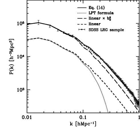
Figure 5: Comparison of the theoretical power spectra and the SDSS LRG power spectrum.The dotted curve is the LPT formula, and the short-dashed curve is the linear theory. The solid curve is the power spectrum multiplied by the correction factor (14). The long-dashed curve is the linear theory multiplied by the constant $b_{0}^{2}$. The cosmological and fitting parameters are described in Table I labelled as model no.1.

Figure 6: Comparison of the BAO features extracted from theoretical models and from the observational data. The dotted curve is the linear theory and the solid curve is the LPT result. The squares with the error bars are the results from the SDSS LRG sample. The chi-squared score for this example is listed in Table I, labelled as model no.1.

III Comparison with the SDSS LRG power spectrum

Now we confront the theoretical predictions with observations. In particular, we use the SDSS LRG sample from data release 6. The SDSS data reduction procedure is the same as described in Ref. Hutsi . Here we utilize the cubic spline fit to consistently construct the smooth component for both the theoretical and the observational power spectra. However, the overall shape of the power spectrum from the LPT formula does not match the observational power spectrum. The power spectrum of the LPT formula shows the exponential suppression at large wave numbers, as is shown in Eq. (2). This feature can be understood as the nonlinear redshift-space distortion Matsubara , the so-called finger-of-God effect, which is automatically formulated in the LPT formalism. This suppression factor matches a phenomenological model of the redshift-space power spectrum on large scales in Ref. ESW . Such discrepancies probably arise from the truncation of higher order perturbations and ignoring the effect of galaxy clustering bias. This might make a systematic error in extracting the BAO consistently. To avoid this, we first construct the theoretical power spectrum by multiplying the LPT power spectrum by the function $b_{0}^{2}e^{\alpha k^{2}}$ so as to match the SDSS LRG power spectrum,

$$P_{\rm fit}(k)=b_{0}^{2}e^{\alpha k^{2}}P_{\rm LPT}^{({\rm s})}(k),$$ (14)

where $b_{0}$ and $\alpha$ are the fitting parameters. Figure 5 demonstrates the example $P_{\rm fit}(k)$, whose parameters are described in Table I, labeled as model no.1. One can see that this fitting function matches the observed power spectrum well. We also note that the BAO signature extracted using $P_{\rm fit}(k)$ is not sensitive to the choice of $b_{0}$ and $\alpha$.

$${\footnotesize\begin{array}[]{c@{\hspace{3.3mm}}c@{\hspace{3.3mm}}c @{\hspace{3.3mm}}c@{\hspace{3.3mm}}c@{\hspace{3.3mm}}c@{\hspace{3.3mm}} c@{\hspace{3.3mm}}c@{\hspace{3.3mm}}c@{\hspace{3.3mm}} c@{\hspace{3.3mm}}c@{\hspace{3.3mm}}c}\hline\cr\hline\cr{\rm No.}\hfil\hskip 9.3894pt&\Omega_{m}\hfil\hskip 9.3894pt&\Omega_{b}\hfil\hskip 9.3894pt&\sigma_{8}\hfil\hskip 9.3894pt&n_{s}\hfil\hskip 9.3894pt&b_{0}\hfil\hskip 9.3894pt&\alpha[h^{-2}{\rm Mpc}^{2}]\hfil\hskip 9.3894pt&\chi^{2}_{\rm lin}\hfil\hskip 9.3894pt&\chi^{2}_{\rm LPT}\hfil\hskip 9.3894pt&\chi^{2}_{\rm simple}\hfil\hskip 9.3894pt&\chi^{2}_{\rm lin-cov}\hfil\hskip 9.3894pt&\chi^{2}_{\rm LPT-cov}\\ \hline\cr 1\hfil\hskip 9.3894pt&0.27\hfil\hskip 9.3894pt&0.046\hfil\hskip 9.3894pt&0.82\hfil\hskip 9.3894pt&0.96\hfil\hskip 9.3894pt&1.7\hfil\hskip 9.3894pt&27.5\hfil\hskip 9.3894pt&15.1\hfil\hskip 9.3894pt&13.7\hfil\hskip 9.3894pt&13.7\hfil\hskip 9.3894pt&28.2\hfil\hskip 9.3894pt&23.0\\[-5.69054pt] 2\hfil\hskip 9.3894pt&0.27\hfil\hskip 9.3894pt&0.048\hfil\hskip 9.3894pt&0.82\hfil\hskip 9.3894pt&0.96\hfil\hskip 9.3894pt&1.7\hfil\hskip 9.3894pt&27.2\hfil\hskip 9.3894pt&13.9\hfil\hskip 9.3894pt&13.0\hfil\hskip 9.3894pt&12.9\hfil\hskip 9.3894pt&26.4\hfil\hskip 9.3894pt&22.1\\[-5.69054pt] 3\hfil\hskip 9.3894pt&0.27\hfil\hskip 9.3894pt&0.044\hfil\hskip 9.3894pt&0.82\hfil\hskip 9.3894pt&0.96\hfil\hskip 9.3894pt&1.7\hfil\hskip 9.3894pt&27.8\hfil\hskip 9.3894pt&16.6\hfil\hskip 9.3894pt&14.5\hfil\hskip 9.3894pt&14.6\hfil\hskip 9.3894pt&30.5\hfil\hskip 9.3894pt&24.1\\[-5.69054pt] 4\hfil\hskip 9.3894pt&0.27\hfil\hskip 9.3894pt&0.046\hfil\hskip 9.3894pt&0.80\hfil\hskip 9.3894pt&0.96\hfil\hskip 9.3894pt&1.75\hfil\hskip 9.3894pt&26.2\hfil\hskip 9.3894pt&15.1\hfil\hskip 9.3894pt&13.7\hfil\hskip 9.3894pt&13.7\hfil\hskip 9.3894pt&28.2\hfil\hskip 9.3894pt&23.1\\[-5.69054pt] 5\hfil\hskip 9.3894pt&0.27\hfil\hskip 9.3894pt&0.046\hfil\hskip 9.3894pt&0.84\hfil\hskip 9.3894pt&0.96\hfil\hskip 9.3894pt&1.65\hfil\hskip 9.3894pt&28.8\hfil\hskip 9.3894pt&15.1\hfil\hskip 9.3894pt&13.7\hfil\hskip 9.3894pt&13.7\hfil\hskip 9.3894pt&28.2\hfil\hskip 9.3894pt&22.9\\[-5.69054pt] 6\hfil\hskip 9.3894pt&0.27\hfil\hskip 9.3894pt&0.046\hfil\hskip 9.3894pt&0.82\hfil\hskip 9.3894pt&0.94\hfil\hskip 9.3894pt&1.7\hfil\hskip 9.3894pt&28.0\hfil\hskip 9.3894pt&14.9\hfil\hskip 9.3894pt&13.5\hfil\hskip 9.3894pt&13.5\hfil\hskip 9.3894pt&28.0\hfil\hskip 9.3894pt&22.7\\[-5.69054pt] 7\hfil\hskip 9.3894pt&0.27\hfil\hskip 9.3894pt&0.046\hfil\hskip 9.3894pt&0.82\hfil\hskip 9.3894pt&0.98\hfil\hskip 9.3894pt&1.7\hfil\hskip 9.3894pt&27.0\hfil\hskip 9.3894pt&15.2\hfil\hskip 9.3894pt&13.8\hfil\hskip 9.3894pt&13.8\hfil\hskip 9.3894pt&28.4\hfil\hskip 9.3894pt&23.2\\[-5.69054pt] 8\hfil\hskip 9.3894pt&0.26\hfil\hskip 9.3894pt&0.046\hfil\hskip 9.3894pt&0.82\hfil\hskip 9.3894pt&0.96\hfil\hskip 9.3894pt&1.65\hfil\hskip 9.3894pt&28.8\hfil\hskip 9.3894pt&15.3\hfil\hskip 9.3894pt&12.5\hfil\hskip 9.3894pt&13.0\hfil\hskip 9.3894pt&29.7\hfil\hskip 9.3894pt&22.3\\[-5.69054pt] 9\hfil\hskip 9.3894pt&0.28\hfil\hskip 9.3894pt&0.046\hfil\hskip 9.3894pt&0.82\hfil\hskip 9.3894pt&0.96\hfil\hskip 9.3894pt&1.75\hfil\hskip 9.3894pt&26.0\hfil\hskip 9.3894pt&15.3\hfil\hskip 9.3894pt&15.0\hfil\hskip 9.3894pt&14.5\hfil\hskip 9.3894pt&27.3\hfil\hskip 9.3894pt&23.8\\ \hline\cr\end{array}}$$ (25)

Table 1: The results of the chi-squared test for the BAO signature for various cosmological models. $\chi^{2}_{\rm LPT}$ is based on the LPT power spectrum, while $\chi^{2}_{\rm lin}$ assumes the linear power spectrum. $\chi^{2}_{\rm simple}$ is the minimum chi-squared value in fitting the model $B(k)=[1-d_{*}^{2}k^{2}]B_{\rm lin}(k)$. $\chi^{2}_{\rm lin-cov}$ and $\chi^{2}_{\rm LPT-cov}$ assume the linear and LPT power spectra, respectively, in evaluating Eq. (27).

Figure 6 compares the BAO signatures extracted from the theoretical models and the SDSS LRG power spectrum of Fig. 5. We computed the chi-square as

$$\chi^{2}=\sum_{i}{[B^{\rm th}(k_{i})-B^{\rm ob}(k_{i})]^{2}\over\Delta B(k_{i})^{2}},$$ (26)

where $B^{\rm th}(k_{i})$ and $B^{\rm ob}(k_{i})$ are the theoretical and observational BAO signatures at wave number $k_{i}$, respectively, and $\Delta B(k_{i})$ is the error. In the computation, we used the data in the wave number range of $0.015\leq k\leq 0.195$. The values of the chi-squared test for various cosmological models are listed in Table I. Here $\chi^{2}_{\rm LPT}$ is the result for the theoretical LPT model, while $\chi^{2}_{\rm lin}$ is that for the linear theory, which does not take the BAO damping into account. In this computation, we have not fitted any parameters, and the number of degrees of freedom is $19$. $\chi^{2}_{\rm LPT}<\chi^{2}_{\rm lin}$ for all of the models. This means that the models with the BAO damping match the observational results better.

As an additional test, we compared the observational BAO signature with a very simple theoretical model $B(k)=[1-d_{*}^{2}k^{2}]B_{\rm lin}(k)$, which includes the leading correction to the damping. Taking $d_{*}$ as a free parameter, we computed the chi-square and we found a minimum value at $d_{*}\simeq 4h^{-1}{\rm Mpc}$, for the models in Table I. $\chi^{2}_{\rm simple}$ is the minimum chi-square. Note that the case $d_{*}=0$ corresponds to the linear theory. Then, $\Delta\chi^{2}=\chi^{2}_{\rm lin}-\chi^{2}_{\rm simple}\sim 1$, which suggests that the detection of the BAO damping is at the 1 sigma level.

To see the effect of the covariance between the data points, we compute

$$\chi_{\rm cov}^{2}=\sum_{i,j}\left[B^{\rm th}(k_{i})-B^{\rm ob}(k_{i})\right]\tilde{P}(k_{i}){\rm Cov}^{-1}(k_{i},k_{j})\tilde{P}(k_{j})\left[B^{\rm th}(k_{j})-B^{\rm ob}(k_{j})\right],$$ (27)

where ${\rm Cov}(k_{i},k_{j})$ is the covariance matrix of the power spectrum. Here the covariance matrix is obtained by using $100$ mock catalogs generated via the second-order Lagrangian perturbation theory and Poisson sampling. The details of the procedure are described in Ref. Hutsi . Figure 7 shows the resulting correlation matrix, which is defined by

$${\rm r}(k_{i},k_{j})={{\rm Cov}(k_{i},k_{j})\over\sqrt{{\rm Cov}(k_{i},k_{i}){\rm Cov}(k_{j},k_{j})}}.$$ (28)

The result of $\chi^{2}_{\rm cov}$ value is shown in Table I, where $\chi_{\rm LPT-cov}{}^{2}$ ($\chi_{\rm lin-cov}{}^{2}$) is the result for the theoretical LPT model (the linear theory). We find $\chi^{2}_{\rm LPT-cov}<\chi^{2}_{\rm lin-cov}$ for all the models, again.

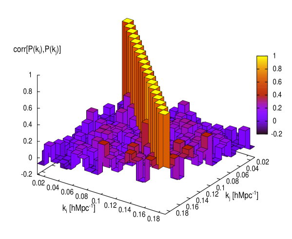
Figure 7: Correlation matrix Hutsi obtained from 100 mock catalogs.

As discussed in Ref.Nomura , to the leading order, the magnitude of the BAO damping is proportional to the amplitude of the matter power spectrum, $D_{1}(z)\sigma_{8}$. Thus, the precise measurement of the BAO damping might be useful in determining $D_{1}(z)\sigma_{8}$. To estimate the minimum achievable error we have computed the diagonal entry for $D_{1}(z)\sigma_{8}$ in the inverse Fisher matrix. For the Fisher matrix calculation we have adopted the same approach as described in Ref. Nomura but here used the angular average of $P({k,\mu},z)$ instead of real space power spectrum. The results are almost the same as those for real space in Ref. Nomura . The minimum attainable error of $D_{1}(z=0.9)\sigma_{8}$ is $\sim 0.1~{}\times\left(\Delta A/2000{\rm deg.}^{2}\right)^{1/2}$ (at the $1$ sigma level), where $\Delta A$ denotes the survey area. In this computation, we assume that the galaxy sample covers the redshift range $0.5\leq z\leq 1.3$, the mean number density of galaxies $n=5.0\times 10^{-4}h^{3}{\rm Mpc}^{-3}$, and the clustering bias $b=2.0$. Note that the error on $D_{1}(z=0.9)\sigma_{8}$ depends on the mean number density of galaxies and the clustering bias Nomura .

IV Summary and Conclusions

In the present work we investigated the influence of the redshift-space distortions on the damping of the BAO in the matter power spectrum. The modeling was based on the work developed by Matsubara, which uses the technique of resuming infinite series of higher order perturbations within the framework of the Lagrangian perturbation theory Matsubara . The result shows that additional BAO damping appears due to redshift-space distortions. We confronted the theoretical BAO signature with the observed power spectrum of the SDSS LRG sample. The chi-squared test suggests that the observed power spectrum favors models with the BAO damping over the ones without the damping. Though the statistical significance is not high, the BAO damping has likely been detected in the SDSS LRG power spectrum. In our modeling we have not taken into account the effect of the clustering bias on the BAO damping. This should be considered more carefully (cf. MatsubaraII ); however, the authors of Ref. SBA show that the BAO damping does not depend much on the halo bias in redshift space.

Acknowledgements This work was supported by a Grant-in-Aid for Scientific research of Japanese Ministry of Education, Culture, Sports, Science and Technology (No. 18540277) TN is supported by a Grant-in-Aid from JSPS (No.DC1: 19-7066).

References

• (1) D. J. Eisenstein and W. Hu, Astrophys. J. 496 605 (1998)
• (2) A. Meiksin, M. White and J. A. Peacock, MNRAS 304 851 (1999)
• (3) D. J. Eisenstein et al, Astrophys. J. 633 560 (2005)
• (4) G. Hütsi, Astron. Astrophys. 449 891 (2006)
• (5) W. J. Percival et al, Astrophys. J. 657 645 (2007)
• (6) W. J. Percival et al, Astrophys. J. 657 51 (2007)
• (7) M. Tegmark et al, Phys. Rev. D 74 123507 (2006)
• (8) K. Yamamoto, Astrophs. J. 595 577 (2003)
• (9) W. J. Percival et al, MNRAS 381 1053 (2007)
• (10) T. Okumura, et al, Astrophys. J. 676 889 (2008)
• (11) G. Hütsi, Astron. Astrophys. 459 375 (2006)
• (12) http://www.sdss3.org/
• (13) B. . Bassett, R. C. Nichol & D. J. Eisenstein, arXiv:astro-ph/0510272
• (14) http://www.lsst.org/
• (15) http://www.skatelescope.org/
• (16) M. Robberto et al, arXiv:0710.3970
• (17) L. Guzzo et al, Nature 451 541 (2008)
• (18) K. Yamamoto, T. Sato and G. Hütsi, Prog. Theor. Phys. 120 609 (2008)
• (19) Y-S. Song and W. J. Percival, arXiv:0807.0810
• (20) H. Nomura, K. Yamamoto and T. Nishimichi, JCAP 0810 031 (2008)
• (21) T. Matsubara, Phys. Rev. D 77 063530 (2008)
• (22) T. Nishimichi et al, Publ. Astron. Soc. Jpn 59 1049 (2007)
• (23) T. Nishimichi et al, arXiv:0810.0813; T. Nishimichi et al, in prep.
• (24) D. J. Eisenstein, H.-J. Seo, and M. White, Astrophys. J. ,664, 660 (2007)
• (25) T. Matsubara, Phys. Rev. D 78 083519 (2008)
• (26) A. G. Sanchez, C. M. Baugh, and R. Angulo, MNRAS 390 1470 (2008)