Breaking down the Fermi acceleration with inelastic collisions

Abstract

The phenomenon of Fermi acceleration is addressed for a dissipative bouncing ball model with external stochastic perturbation. It is shown that the introduction of energy dissipation (inelastic collisions of the particle with the moving wall) is a sufficient condition to break down the process of Fermi acceleration. The phase transition from bounded to unbounded energy growth in the limit of vanishing dissipation is characterized.

The phenomenon of Fermi acceleration (FA) is a process in which a classical particle acquires unbounded energy from collisions with a heavy moving wall [1]. This phenomenon was originally proposed by Enrico Fermi [2] as a possible explanation for the origin of the large energies of cosmic particles. His original model was later modified by several investigators and applied in several fields of physics, including plasma physics [3], astrophysics [4, 5], atomic physics [6], optics [7, 8, 9] and the well known time-dependent billiard problems [10, 11]. Since the seminal paper of Hammersley [12], it is known that the particle’s average energy grows with time when there is a random perturbation at each impact with the wall. This result was also confirmed for a stochastic version of the one-dimensional bouncing ball model (a classical particle confined in and hitting two rigid walls; one of them with a fixed position and the other one with periodic movement) under the framework of random shift perturbation [13, 14].

One of the most important questions on Fermi acceleration is whether it can result from the nonlinear dynamics in the absence of a random component. The answer to this question depends on the model under consideration. For example, for a bouncer model (a particle hitting a periodically moving platform in the presence of a constant gravitational field), there are specific ranges of control parameters and initial conditions that lead to Fermi acceleration [15]; FA occurs when there are no invariant spanning curves on the phase space limiting the chaotic sea and, consequently, the particle’s energy gain [13, 14]. For two-dimensional time-dependent billiards (billiards with moving boundaries), the emergence of FA depends on the type of phase space of the corresponding static version of the problem [16]. Therefore, as conjectured by Loskutov and collaborators [16], the chaotic dynamics of a particle for static boundary is a sufficient condition to produce FA if a time perturbation in the boundary is introduced.

A second and very important question is: in the classical billiard problems where FA is present, are inelastic collisions of the particle with the boundaries a sufficient condition to suppress the unlimited energy gain?

In this Letter, we consider the one-dimensional Fermi accelerator model under stochastic perturbation and we seek to understand and describe a mechanism to suppress the FA. The model consists of a classical particle confined to bounce between two rigid and infinitely heavy walls. One of them is fixed while the other one moves randomly with dimensionless amplitude of motion $\epsilon$ [17]. It is assumed that collisions with the moving wall are inelastic, so that the particle experiences a fractional loss of energy upon each collision. A restitution coefficient $\alpha\in[0,1]$ controls the strength of the dissipation. For $\alpha=1$, all collisions are elastic and therefore FA is observed [15]. On the other hand, for $\alpha<1$ the model is dissipative and, as shown here, there is a bound to the energy growth. In other words, inelastic collisions break down the FA process. A phase transition from bounded to unbounded energy growth is observed when the control parameter $\alpha$ approaches the unity. Here we investigate this phase transition by studying the limit $\alpha\rightarrow 1$. The present approach can be useful as a mechanism to subdue the phenomenon of FA in time-dependent billiard problems.

The dynamics of the problem is given by a two-dimensional, nonlinear mapping for the particle velocity $V$ and the time $t$ at each impact of the particle with the moving wall. We investigate in this Letter a simplified version of the model [13, 14, 18, 19, 20] which speeds up the numerical simulations significantly without affecting the universality class. However, similar results would indeed be obtained for the full model. The simplified version assumes that both walls are fixed but that, when the particle hits one of them, it exchanges energy and momentum as if the wall were moving randomly. Thus, considering dimensionless variables and taking into account the inelastic collisions, the mapping that describes the dynamics of the model is

$$\left\{\begin{array}[]{ll}V_{n+1}=|\alpha V_{n}-(1+\alpha)\epsilon\sin(\phi_{n+1})|\\ \phi_{n+1}=\phi_{n}+{{2}\over{V_{n}}}+Z(n)~{}~{}{\rm mod}~{}~{}2\pi\\ \end{array}\right.~{},$$ (1)

where $n$ is the iteration number and $Z(n)\in[0,2\pi)$ corresponds to a random shift in the phase of the moving wall. It is clear that the model has two control parameters, namely $\epsilon$ and $\alpha$, whose effect must be considered.

The most natural observable in problems involving FA is the average velocity, which is calculated here in two steps. The first step consists in averaging the velocity over the orbit for a single initial condition. It is defined as

$$V_{i}(n,\epsilon,\alpha)={{1}\over{n+1}}\sum_{j=0}^{n}V_{j,i}~{},$$ (2)

where the index $j$ refers to the $j$th iteration of the sample $i$. The second step is to calculate the average over an ensemble of $M$ different initial conditions

$${\overline{V}}={{1}\over{M}}\sum_{i=1}^{M}V_{i}~{}.$$ (3)

The behavior of the average velocity ${\overline{V}}$ for different values of the control parameters is shown in Fig. 1.

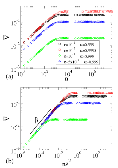
Figure 1: (Color online) (a) Behavior of ${\overline{V}}$ as a function of the iteration number $n$ for different values of the control parameters $\epsilon$ and $\alpha$. (b) Curves shown in (a) after the change of variables $n\rightarrow n\epsilon^{2}$.

Note that the growth of ${\overline{V}}$ with $n$ is described by different curves for different values of $\epsilon$ (Fig. 1(a)). However, a transformation $n\rightarrow n\epsilon^{2}$ coalesces all curves, so that they grow together for small $n$, as seen in Fig. 1(b). Also, instead of studying the behavior of ${\overline{V}}$ as a function of the damping coefficient $\alpha$, we adopt the variable $(1-\alpha)$ in order to bring the transition to the origin. Such a transformation improves visualization in log-log plots.

Let us now discuss the behavior observed in Fig. 1. It is easy to see that all curves start growing together for small iteration numbers and then they bend towards a regime of convergency. Such a regime is marked by a constant plateau for the average velocity. The change from growth to saturation is characterized by a typical crossover iteration number $n_{x}$. Based on the results seen in Fig. 1, one concludes that the velocity grows as a power law of the type ${\overline{V}}\propto(n\epsilon^{2})^{\beta}$ for $n\ll n_{x}$. For large iteration numbers, the saturation velocity for a fixed damping coefficient $\alpha$ is given by ${\overline{V}}_{\rm sat}\propto\epsilon^{\alpha_{1}}$. On the other hand, for a fixed $\epsilon$, the values obtained are ${\overline{V}}_{\rm sat}\propto(1-\alpha)^{\alpha_{2}}$. The typical crossover iteration number that marks the transition from growth to the saturation is assumed to be of the following form: (i) for a constant $\alpha$, $n_{x}\epsilon^{2}\propto\epsilon^{z_{1}}$ and; (ii) for a fixed $\epsilon$, $n_{x}\epsilon^{2}\propto(1-\alpha)^{z_{2}}$. These initial assumptions allow us to propose the following scaling hypotheses:

• For small iteration numbers ($n\ll n_{x}$), the average velocity grows as

  $${\overline{V}}\propto[n\epsilon^{2}]^{\beta}~{},$$ (4)

  where $\beta$ is a critical exponent.

• For large iteration numbers ($n\gg n_{x}$), the constant plateau of the velocity is given by

  $${\overline{V}}_{\rm sat}\propto\epsilon^{\alpha_{1}}(1-\alpha)^{\alpha_{2}}~{},$$ (5)

  where both $\alpha_{1}$ and $\alpha_{2}$ are critical exponents.

• The crossover iteration number is given by

  $$n_{x}\epsilon^{2}\propto\epsilon^{z_{1}}(1-\alpha)^{z_{2}}~{},$$ (6)

  with $z_{1}$ and $z_{2}$ being the dynamical exponents.

These three hypotheses allow us to formally describe the average velocity using a scaling function of the type

$${\overline{V}}(n\epsilon^{2},\epsilon,(1-\alpha))=l{\overline{V}}(l^{a}n\epsilon^{2},l^{b}\epsilon,l^{c}(1-\alpha))~{},$$ (7)

where $l$ is a scaling factor and $a$, $b$ and $c$ are the scaling exponents which must be related to the critical exponents $\beta$, $\alpha_{1}$ and $\alpha_{2}$, $z_{1}$ and $z_{2}$. Since $l$ is a scaling factor, we can choose $l=[n\epsilon^{2}]^{-1/a}$. Using this expression for $l$, Eq. (7) is rewritten as

$${\overline{V}}(n\epsilon^{2},\epsilon,(1-\alpha))=[n\epsilon^{2}]^{-{{1}\over{a}}}V_{1}([n\epsilon^{2}]^{-{{b}\over{a}}}\epsilon,[n\epsilon^{2}]^{-{{c}\over{a}}}(1-\alpha))~{},$$ (8)

where the function $V_{1}$ is assumed to be constant for $n\ll n_{x}$. Comparing equations (8) and (4), we obtain $\beta=-1/a$. After conducting extensive numerical simulations, it was found that $\beta=0.494(1)\cong 0.5$, which implies $a=-2$. Let us now consider the case $n\gg n_{x}$. This case allows us to choose two distinct values for $l$, namely: (a) $l=\epsilon^{-1/b}$ and (b) $l=(1-\alpha)^{-1/c}$. For case (a), the scaling function is rewritten as

$${\overline{V}}(n\epsilon^{2},\epsilon,(1-\alpha))=\epsilon^{-{{1}\over{b}}}V_{2}(\epsilon^{-{{a}\over{b}}}n\epsilon^{2},\epsilon^{-{{c}\over{b}}}(1-\alpha))~{},$$ (9)

with the function $V_{2}$ being constant for $n\gg n_{x}$ and $\alpha$ constant. A comparison of equations (9) and (5) furnishes $\alpha_{1}=-1/b$. After fitting a power law to data on the plot ${\overline{V}}_{\rm sat}\times\epsilon$, we find $\alpha_{1}=1.0011(2)\cong 1$ (see Fig. 2(a)), which provides $b=-1$.

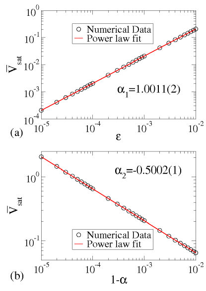
Figure 2: (Color online) (a) Plot of ${\overline{V}}_{\rm sat}\times\epsilon$. A power law fitting gives $\alpha_{1}=1.0011(2)$. (b) Plot of ${\overline{V}}_{\rm sat}\times(1-\alpha)$. The exponent obtained via a power-law fitting is $\alpha_{2}=-0.5002(1)$.

We now have to consider case (b), i.e., $l=(1-\alpha)^{-1/c}$. Using this scaling factor, Eq. (7) is given by

$${\overline{V}}(n\epsilon^{2},\epsilon,(1-\alpha))=(1-\alpha)^{-{{1}\over{c}}}V_{3}((1-\alpha)^{-{{a}\over{c}}}n\epsilon^{2},(1-\alpha)^{-{{b}\over{c}}}\epsilon)$$ (10)

where we assume that $V_{3}$ is constant for $n\gg n_{x}$ and $\epsilon$ constant. Comparing equations (10) and (5), it is easy to see that $\alpha_{2}=-1/c$. A power-law fitting to the data for ${\overline{V}}_{\rm sat}\times(1-\alpha)$ gives that $\alpha_{2}=-0.5002(1)\cong-0.5$, yielding $c=2$.

Considering the different expressions for the scaling factor $l$ obtained for $n\ll n_{x}$ and case (a) of $n\gg n_{x}$, we obtain

$$n\epsilon^{2}=\epsilon^{{a}\over{b}}~{}.$$ (11)

A comparison of equations (11) and (6) provides $z_{1}=a/b$. Fitting a power law to the data on the plot $n_{x}\epsilon^{2}\times\epsilon$ furnishes $z_{1}=2.001(2)$, as shown in Fig. 3(a).

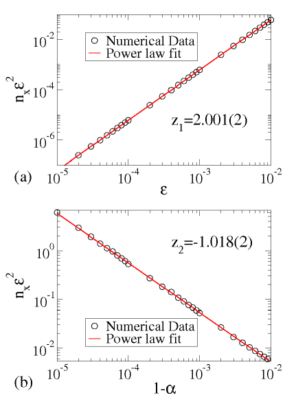
Figure 3: (Color online) (a) Plot of $n_{x}\epsilon^{2}\times\epsilon$. After fitting a power law we obtain that $z_{1}=2.001(2)$. (b) Plot of $n_{x}\epsilon^{2}\times(1-\alpha)$ for a fixed $\epsilon=10^{-2}$. Fitting a power law, we find $z_{2}=-1.018(2)$.

This result is in agreement with the ratio $a/b=2$. As a next step, we consider the case of the different expressions for the scaling factor $l$ obtained for $n\ll n_{x}$ and case (b) of $n\gg n_{x}$. Such procedure gives

$$n\epsilon^{2}=(1-\alpha)^{{a}\over{c}}~{}.$$ (12)

Comparing equations (12) and (6), we obtain that $z_{2}=a/c$. A power-law fitting to the data on the plot $n_{x}\epsilon^{2}\times(1-\alpha)$ (Fig. 3(b)), with $\epsilon=10^{-2}$, gives $z_{2}=-1.018(2)$. This result is also in good agreement with the result obtained from $a/c=-1$.

Let us now discuss the consequences of the critical exponents $\alpha_{2}$ and $z_{2}$ on the FA. It is clear that, in the limit $\alpha\rightarrow 1$, both Eqs. (5) and (6) diverge. Therefore, in the limit of vanishing dissipation, the average velocity ${\overline{V}}$ and the crossover iteration number $n_{x}$ diverge. This is a clear signature of a phase transition from bounded to unbounded energy growth. Finally, in order to check the validity of the scaling hypotheses, we can now proceed to collapse all the curves onto a single and universal plot, as shown in Fig. 4.

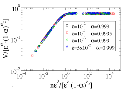
Figure 4: (Color online) Collapse of the curves shown in Fig. 1(b) onto a single and universal plot.

In summary, the problem of a stochastic bouncing ball model with inelastic collisions is addressed. It is shown that, when dissipation is present, the average velocity of a classical particle grows with time and then reaches a regime of saturation. However, in the limit of vanishing dissipation, the phenomenon of Fermi acceleration is recovered. Similar results were also observed for a dissipative and deterministic bouncer model [21, 22]. These results allow us to propose the following conjecture: For one-dimensional billiard problems that show unlimited energy growth for both their deterministic and stochastic dynamics, the introduction of inelastic collision in the boundaries is a sufficient condition to break down the phenomenon of Fermi acceleration. Such phenomenon is also expected to be observed in two-dimensional, time-varying billiard problems since the FA mechanism is the same as that of the one-dimensional case.

E.D.L. thanks Prof. P.V.E. McClintock for fruitful discussions and Dr. G.J.M. Garcia for a careful review of the manuscript. Support from CNPq, FAPESP and FUNDUNESP, Brazilian agencies, is gratefully acknowledged.

References

References

- [1] Ulam S 1961 Proceedings of the Fourth Berkeley Symposium on Math. Statistics and Probability Vol 1 315 (University of California Press, Berkeley)
- [2] Fermi E 1949 Phys. Rev 75 1169
- [3] Milovanov A V, Zelenyi L M 2001 Phys. Rev. E 64 052101
- [4] Veltri A, Carbone V 2004 Phys. Rev. Lett. 92 143901
- [5] Kobayakawa K, Honda Y S, Samura T 2002 Phys. Rev. D 66 083004
- [6] Lanzano G et al. 1999 Phys. Rev. Lett. 83 4518
- [7] Saif F, Bialynicki-Birula I, Fortunato M, Schleich W P 1998 Phys. Rev. A 58 4779
- [8] Saif F, Rehman I 2007 Phys. Rev. A 75 043610
- [9] Steane A, Szriftgiser P, Desbiolles P, Dalibard J 1995 Phys. Rev. Lett. 74 4972
- [10] Loskutov A, Ryabov A B 2002 J. Stat. Phys. 108 995
- [11] Egydio de Carvalho R, de Sousa F C, Leonel E D 2006 J. Phys. A 39 3561
- [12] Hammersley J M 1961 Proceedings of the Fourth Berkeley Symposium on Math. Statistics and Probability Vol 1 79 (University of California Press, Berkeley)
- [13] Karlis A K, Papachristou P K, Diakonos F K, Constantoudis V, Schmecher P 2006 Phys. Rev. Lett. 97 194102
- [14] Karlis A K, Papachristou P K, Diakonos F K, Constantoudis V, Schmecher P 2007 Phys. Rev. E 76 016214
- [15] Lichtenberg A J, Lieberman M A, Cohen R H 1980 Physica D 1 291
- [16] Loskutov A, Ryabov A B, Akinshin L G 2000 J. Phys. A 33 7973
- [17] This is an artificial mechanism commonly used to produce Fermi acceleration in billiard problems. See for example Refs. [13, 14].
- [18] Lichtenberg A J, Lieberman M A 1992 Regular and Chaotic Dynamics (Appl. Math. Sci. 38 Springer Verlag, New York)
- [19] Leonel E D, McClintock P V E 2005 J. Phys. A 38 823
- [20] Ladeira D G, da Silva J K L 2006 Phys. Rev. E 73 026201
- [21] Leonel E D, Livorati A L P 2007 Unpublished
- [22] Ladeira D G, Leonel E D 2007 Unpublished