Nonperturbative Effect in Threshold Resummation

Abstract:

We show that the conventional threshold resummation calculation cannot describe well the low energy Drell-Yan (DY) data without including the non-perturbative correction terms which are deduced from analyzing the asymptotic behavior of the resummation formalism. It is demonstrated that the non-perturbative correction is generally small for the large invariant mass DY pairs produced at the Tevatron and the LHC.

1 Introduction

With ample data accumulated at the Fermilab Tevatron and expected at the up-coming CERN Large Hadron Collider (LHC), precision measurements at hadron colliders become possible. To test the Standard Model (SM) predictions and to probe possible new physics signatures, many higher order theoretical calculations have been performed in recent years to study the phenomenology of Drell-Yan (DY) pair, $W$ boson, top quark pair and Higgs boson produced in hadron collisions. It is well known that in perturbative QCD (pQCD) hadronic cross sections could receive logarithmically enhanced contribution in the partonic threshold region, which corresponds to $z\to 1$, where $z=Q^{2}/\hat{s}$ with $Q$ being the invariant mass of the final state (say, the DY pair) and $\sqrt{\hat{s}}$ the center-of-mass (CM) energy of the partonic process. These contributions take the form of “plus” distributions, such as $[\ln^{n}(1-z)/(1-z)]_{+}$, and can be resummed to all orders in the expansion of the strong coupling $\alpha_{s}$. This is called the threshold resummation calculation which plays an important role for precision tests at hadron colliders.

A typical Sudakov exponent in threshold resummation [1] in the modified minimal subtraction ($\overline{\text{MS}}$) [2, 3] scheme,

$$\begin{split}E^{f_{i}}(N)=&-\int_{0}^{1}dz\frac{z^{N-1}-1}{1-z}\Big{\{}\int_{(1-z)^{2}}^{1}\frac{d\lambda}{\lambda}A^{(f_{i})}[\alpha_{s}(\lambda Q^{2})]+\nu^{(f_{i})}[\alpha_{s}((1-z)^{2}Q^{2})]\Big{\}}\end{split}\,,$$ (1)

generally involves singularities, known as the Landau pole of QCD running coupling. This occurs when the relevant energy scale is smaller than the QCD scale $\Lambda_{\text{QCD}}$, as $z\to 1$ or $\lambda\to 0$, where the pQCD fails and the non-perturbative QCD effects must set in. To avoid directly confronting the non-perturbative contribution, a few approaches have been proposed in the literature. One approach is to apply the principal value resummation [4] to choose a contour to evaluate the above integral without hitting Landau pole [1, 4, 5]. Another method to treat the Landau pole problem was recently proposed by Bonvini et al. in Ref. [6]. Other approaches were also proposed in the literature. For example, in Ref. [7], Becher et al. established an approach to resum the logarithmic contributions directly in the momentum space based on effective theory. In Ref. [8], Kidonakis et al. proposed to approximate the resummation calculation by an expansion of the resummed cross section, which will be further discussed below. In this paper, we propose a new approach to add non-perturbative correction terms to the minimal prescription threshold resummation formalism [5], as suggested by the perturbative expansion of joint resummation.

This paper is organized as follows. In Section 2 we shall first briefly review the relevant part of threshold resummation (RES) formalism. In Section 3 from the threshold resummation formalism we induce the functional form of the non-perturbative (NP) correction terms to be added to the minimal prescription threshold resummation calculation. Then, in Section 4 we apply this new threshold resummation formalism, denoted here as RES+NP, to three DY experiments with CM energy of the hadron colliders ranging from 38.76 GeV to 1960 GeV [9, 10, 11]. From the comparison to data, we determine the coefficients in the NP correction terms of the threshold resummation formalism. We also compare the RES+NP result with the predictions of several popular approaches. Finally, we give our prediction for the DY pair production at the LHC. Section 5 contains a brief summary of the conclusions.

2 Threshold Resummation

The differential cross section of the DY pair, in terms of its invariant mass ($Q$) and rapidity ($Y$), in the hadron CM frame (with energy $\sqrt{S}$) is [12]

$$\begin{split}S\frac{d\sigma^{H_{1}H_{2}}}{dQ^{2}dY}(\tau,Y)=&\int_{0}^{1}dz\int^{1}_{0}\frac{dx_{1}}{x_{1}}\int^{1}_{0}\frac{dx_{2}}{x_{2}}f_{p_{1}}^{H_{1}}(x_{1},\mu_{F})f_{p_{2}}^{H_{2}}(x_{2},\mu_{F})\delta(z-\frac{\tau}{x_{1}x_{2}})\frac{d\sigma^{p_{1}p_{2}}}{dzdy}(z,y),\end{split}$$ (2)

where $\tau={Q^{2}}/{S}$. $y$ is the rapidity of lepton pair in the parton CM frame. $f_{p_{i}}^{H_{i}}$ are the parton distribution functions (PDFs), and $\mu_{F}$ is the factorization scale.

Conventionally, the rapidity-integrated cross sections only need the Mellin transform to turn the convolution into multiplication. However, for the case of the rapidity distribution the Fourier transform with respect to $Y$ is also needed [13, 14]. Applying the Mellin-Fourier transform to Eq.(2), we obtain

$$\begin{split}\widetilde{\omega}^{H_{1}H_{2}}&\equiv\int_{0}^{1}d\tau\tau^{N-1}\int_{\ln\sqrt{\tau}}^{-\ln\sqrt{\tau}}dYe^{iMY}S\frac{d\sigma^{H_{1}H_{2}}}{dQ^{2}dY}(\tau,Y)\\ &=\widetilde{f}_{p_{1}}^{H_{1}}(N+iM/2)\widetilde{f}_{p_{2}}^{H_{2}}(N-iM/2)\widetilde{\omega}^{p_{1}p_{2}},\end{split}$$ (3)

where

$$\widetilde{f}_{p_{i}}^{H_{i}}(N\pm iM/2)=\int_{0}^{1}dxx^{N-1\pm iM/2}f_{p_{i}}^{H_{i}}(x_{i})$$ (4)

and

$$\widetilde{\omega}^{p_{1}p_{2}}(N,M)=\int_{0}^{1}dzz^{N-1}\int_{\ln\sqrt{z}}^{-\ln\sqrt{z}}dye^{iMy}\frac{d\sigma^{p_{1}p_{2}}}{dzdy}$$ (5)

are the PDFs and differential cross section in moment space, respectively. As shown in Ref. [13], near threshold region the $M$ dependence in $\widetilde{\omega}^{p_{1}p_{2}}(N,M)$ is negligible, and it is a good approximation to take the well-known resummed form [3, 13] for the rapidity-integrated cross section,

$$\begin{split}\widetilde{\omega}^{p_{1}p_{2}}_{\text{res}}(N,M)&\approx\widetilde{\omega}^{p_{1}p_{2}}_{\text{res}}(N)=\exp\Big{[}\sum_{i}E^{p_{i}}(N)\Big{]}\exp\Big{[}\sum_{i}2\int_{\mu_{F}}^{Q}\frac{d\mu}{\mu}\gamma_{p_{i}/p_{i}}(\alpha_{s}(\mu^{2}))\Big{]}\\ &\times\text{Tr}\Big{\{}H^{p_{1}p_{2}}(\alpha_{s}(\mu_{R}^{2}))\bar{P}\exp\Big{[}\int_{Q}^{Q/\tilde{N}}\frac{d\mu}{\mu}\Gamma^{\dagger p_{1}p_{2}}_{S}(\alpha_{s}(\mu^{2}))\Big{]}\\ &\times\tilde{S}^{p_{1}p_{2}}\Big{(}1,\alpha_{s}\Big{(}\frac{Q^{2}}{\tilde{N}^{2}}\Big{)}\Big{)}P\exp\Big{[}\int_{Q}^{Q/\tilde{N}}\frac{d\mu}{\mu}\Gamma_{S}^{p_{1}p_{2}}(\alpha_{s}(\mu^{2}))\Big{]}\Big{\}},\end{split}$$ (6)

where $\tilde{N}=N\exp{(\gamma_{E})}$, $\gamma_{E}$ is the Euler constant, and $\mu_{R}$ is the renormalization scale. $P$ denotes path ordering [15]. The first exponent in Eq.(6), as given in Eq. (1), resums the collinear and soft gluon emission contributions from the initial state, with

$$A^{(f_{i})}(\alpha_{s})=C_{f}\Big{(}\frac{\alpha_{s}}{\pi}+\frac{1}{2}K\Big{(}\frac{\alpha_{s}}{\pi}\Big{)}^{2}\Big{)},$$ (7)

$$K=C_{A}\Big{(}\frac{67}{18}-\frac{\pi^{2}}{6}\Big{)}-\frac{5}{9}n_{f},$$ (8)

$$\nu^{(f_{i})}(\alpha_{s})=\frac{2C_{f}}{\pi}\alpha_{s},$$ (9)

where $n_{f}$ is the flavor number of light quarks. $C_{f}=C_{F}=(N_{c}^{2}-1)/(2N_{c})$ for initial state quarks and $C_{f}=C_{A}=N_{c}$ for initial state gluons. $N_{c}$ is the number of colors. In Eq.(6), at the one-loop order, $\gamma_{q/q}=(\alpha_{s}/\pi)(\frac{3}{4}C_{F}-C_{F}\ln\tilde{N})$ for quarks, and $\gamma_{g/g}=(\alpha_{s}/\pi)(\beta_{0}-C_{A}\ln\tilde{N})$ for gluons. The $\beta$ function is defined as

$$\beta(\alpha_{s})=\frac{1}{2}\mu\frac{d\ln g_{s}}{d\mu}=-\sum_{n=0}^{\infty}\beta_{n}\Big{(}\frac{\alpha_{s}}{\pi}\Big{)}^{(n+2)},$$ (10)

with

$$\beta_{0}=(11C_{A}-2n_{f})/12,$$ (11)

$$\beta_{1}=(17C_{A}^{2}-5C_{A}n_{f}-3C_{F}n_{f})/24.$$ (12)

$\Gamma_{S}$ in Eq.(6) is the soft anomalous dimension matrix, which can be derived from the eikonal diagrams [1, 3] and is given at the one-loop order by

$$\Gamma_{S}=\frac{\alpha_{s}C_{F}}{\pi}(1-\pi i).$$ (13)

At the next-to-leading logarithm (NLL) accuracy, $\widetilde{\omega}^{p_{1}p_{2}}$ is approximated as [13]

$$\widetilde{\omega}^{p_{1}p_{2}}_{\text{NLL}}(N)=\widetilde{\omega}^{p_{1}p_{2}}_{B}C(\alpha_{s})\exp[g_{1}(\lambda)\ln\tilde{N}+g_{2}(\lambda)],$$ (14)

with

$$\lambda=\beta_{0}\alpha_{s}\ln\tilde{N}/\pi,$$ (15)

$$g_{1}(\lambda)=\frac{C_{F}}{\beta_{0}\lambda}\Big{[}2\lambda+(1-2\lambda)\ln(1-2\lambda)\Big{]},$$ (16)

$$\begin{split}g_{2}(\lambda)&=\frac{C_{F}\beta_{1}}{\beta_{0}^{3}}\Big{[}2\lambda+\ln(1-2\lambda)+\frac{1}{2}\ln^{2}(1-2\lambda)\Big{]}-\frac{C_{F}K}{2\beta_{0}^{2}}[2\lambda+\ln(1-2\lambda)]\\ &+\frac{C_{F}}{\beta_{0}}[2\lambda+\ln(1-2\lambda)]\ln\frac{Q^{2}}{\mu_{R}^{2}}-\frac{C_{F}}{\beta_{0}}2\lambda\ln\frac{Q^{2}}{\mu_{F}^{2}},\end{split}$$ (17)

where $\widetilde{\omega}^{p_{1}p_{2}}_{B}$ is the Born differential cross section in moment space. By matching the moments of the NLO cross section, the coefficient $C(\alpha_{s})$ in Eq.(14) can be obtained as follows [13]

$$C(\alpha_{s})=1+\frac{\alpha_{s}}{\pi}C_{F}\Big{(}-4+\frac{2\pi^{2}}{3}+\frac{3}{2}\ln\frac{Q^{2}}{\mu_{F}^{2}}\Big{)}.$$ (18)

The cross section in momentum space can be obtained via inverse Mellin-Fourier transform

$$\omega^{p_{1}p_{2}}(z,y)=\frac{1}{2\pi i}\int_{C-i\infty}^{C+i\infty}dNz^{-N}\frac{1}{2\pi}\int_{-\infty}^{\infty}dMe^{-iMy}\widetilde{\omega}^{p_{1}p_{2}}(N,M).$$ (19)

In order to avoid double-counting the fixed order contributions up to the next-to-leading order (NLO), it is needed to subtract the first two orders of $\alpha_{s}$ expansion to obtain the final cross section, i.e.,

$$\begin{split}S\frac{d\sigma^{H_{1}H_{2}}_{\text{RES}}}{dQ^{2}dY}&=S\frac{d\sigma^{H_{1}H_{2}}_{\text{NLO}}}{dQ^{2}dY}+S\frac{d\sigma^{H_{1}H_{2}}_{\text{NLL}}}{dQ^{2}dY}-\Big{(}S\frac{d\sigma^{H_{1}H_{2}}_{\text{NLL}}}{dQ^{2}dY}\Big{)}_{\alpha_{s}=0}-\alpha_{s}\Big{(}\frac{\partial}{\partial\alpha_{s}}S\frac{d\sigma^{H_{1}H_{2}}_{\text{NLL}}}{dQ^{2}dY}\Big{)}_{\alpha_{s}=0}\,,\end{split}$$ (20)

where $\sigma^{H_{1}H_{2}}_{\text{NLO}}$, corresponding to $\omega^{p_{1}p_{2}}_{\text{NLO}}$ in the momentum space, denotes the NLO cross section.

For comparison, in this paper we also investigate the next-to-next-to-leading order (NNLO) expansion [8, 16] of the resummed cross sections. At first, in order to reproduce the fixed order expressions, we recover the $M$ dependence in

$$\widetilde{\omega}^{p_{1}p_{2}}(N,M)=\frac{1}{2}[\widetilde{\omega}^{p_{1}p_{2}}(N+iM/2)+\widetilde{\omega}^{p_{1}p_{2}}(N-iM/2)],$$ (21)

although we have neglected the $M$ dependence in the numerical evaluation of the resummed cross section [13]. For the inverse Mellin-Fourier transform of the logarithms $\ln^{k}(N\pm iM/2)$ we find

$$I_{0}= \frac{1}{2\pi i}\int_{C-i\infty}^{C+i\infty}dNz^{-N}\frac{1}{2\pi}\int_{-\infty}^{\infty}dMe^{-iMy}$$

$$= \delta(1-z)\delta(y)$$

$$= \delta(1-z)\delta(y\pm\frac{1}{2}\ln z)$$

$$= \frac{1}{2\pi i}\int_{C-i\infty}^{C+i\infty}dNz^{-N}\delta(y\pm\frac{1}{2}\ln z),$$ (22)

$$I_{k}= \frac{1}{2\pi i}\int_{C-i\infty}^{C+i\infty}dNz^{-N}\frac{1}{2\pi}\int_{-\infty}^{\infty}dMe^{-iMy}[\ln^{k}(N\pm iM/2)+\gamma_{E}]$$

$$= \frac{1}{2\pi i}\int_{C-i\infty}^{C+i\infty}dN^{\prime}z^{-N^{\prime}}\frac{1}{2\pi}\int_{-\infty}^{\infty}dMe^{-iM(y\pm\frac{1}{2}\ln z)}[\ln^{k}(N^{\prime})+\gamma_{E}]$$

$$= \frac{1}{2\pi i}\int_{C-i\infty}^{C+i\infty}dNz^{-N}\ln^{k}(\tilde{N})\delta(y\pm\frac{1}{2}\ln z).$$ (23)

Hence, we can replace the inverse Fourier transform and $M$ dependence by the function $[\delta(y+\frac{1}{2}\ln z)+\delta(y-\frac{1}{2}\ln z)]/2$. The remaining calculation is the same as the rapidity-integrated differential cross section. If we expand the exponent of the resummed cross section in Eq.(14) to the NLO accuracy [16], the differential cross section for DY assuming $\mu_{F}=\mu_{R}=Q$ is

$$\omega^{p_{1}p_{2}(1)}_{\text{exp.}}(z,y)=\omega^{p_{1}p_{2}}_{0}\frac{\alpha_{s}}{\pi}[c_{3}D_{1}(z)+c_{1}\delta(1-z)]\frac{\delta(y+\frac{1}{2}\ln z)+\delta(y-\frac{1}{2}\ln z)}{2},$$ (24)

where $D_{k}(z)=[\ln^{k}(1-z)/(1-z)]_{+}$, $c_{3}=4C_{F}$ and $c_{1}=2C_{F}\zeta_{2}-4C_{F}$. $\omega^{p_{1}p_{2}}_{0}$ is the coefficient of $\delta(1-z)\delta(y)$ in the Born differential cross section $\omega^{p_{1}p_{2}}_{B}$. It is evident that this reproduces the dominant contribution near threshold in the NLO differential cross section, as given in Ref. [17]. Similarly, at the NNLO accuracy, the expansion of the exponent in Eq. (14) yields

$$\begin{split}\omega^{p_{1}p_{2}(2)}_{\text{exp.}}(z,y)=&\omega^{p_{1}p_{2}}_{0}\Big{(}\frac{\alpha_{s}}{\pi}\Big{)}^{2}\Big{\{}\frac{1}{2}c_{3}^{2}D_{3}(z)-\beta_{0}c_{3}D_{2}(z)+(c_{3}c_{1}-\zeta_{2}c_{3}^{2}+2C_{F}K)D_{1}(z)\\ &+(\zeta_{3}c_{3}^{2}-2\beta_{0}c_{1})D_{0}(z)+(\frac{1}{2}c_{1}^{2}+\frac{1}{4}\zeta_{2}^{2}c_{3}^{2}-\frac{3}{4}\zeta_{4}c_{3}^{2})\delta(1-z)\Big{\}}\\ &\times\frac{\delta(y+\frac{1}{2}\ln z)+\delta(y-\frac{1}{2}\ln z)}{2}.\end{split}$$ (25)

Below, we define the NNLO-NLL (next-to-next-to-leading order and next-to-leading logarithmic) [18] corrected differential cross section as

$$\omega^{p_{1}p_{2}}_{\text{NNLO-NLL}}=\omega^{p_{1}p_{2}}_{\text{NLO}}+\omega^{p_{1}p_{2}(2)}_{\text{exp.}}.$$ (26)

3 Nonperturbative Effect

While deriving Eq.(14) from Eq.(1), approximation [5] has been made to avoid Landau pole in the original expansion, and the integration in Eq.(1) was carried out via perturbative expansion. This approximation could fail if the NP contribution in Eq.(1) is large. Hence, we propose to add NP correction terms in the resummation formalism to better approximate the total contribution from Eq.(1). To find out the proper functional form to parameterize the NP corrections, we examine the joint resummation formalism in Ref. [19], where the resummed cross section in moment (and impact parameter) space is expressed as

$$\hat{\sigma}_{ab}^{(eik)}(N,b)=\exp[D_{ab}^{(eik)}(N,b)]\exp[E_{ab}^{(eik)}(N,b)],$$ (27)

where

$$\begin{split}E_{ab}^{(eik)}(N,b)=&\int_{0}^{Q^{2}}\frac{dk_{T}^{2}}{k_{T}^{2}}\Big{\{}\sum_{i=a,b}A_{i}(\alpha_{s}(k_{T}))\Big{[}J_{0}(bk_{T})K_{0}\Big{(}\frac{2Nk_{T}}{Q}\Big{)}+\ln\Big{(}\frac{\tilde{N}k_{T}}{Q}\Big{)}\Big{]}\Big{\}}\\ &-\ln\tilde{N}\int_{\mu_{F}^{2}}^{Q^{2}}\frac{dk_{T}^{2}}{k_{T}^{2}}\sum_{i=a,b}A_{i}(\alpha_{s}(k_{T})),\end{split}$$ (28)

$$\begin{split}D_{ab}^{(eik)}(N,b)=&\int_{0}^{Q^{2}}dk_{T}^{2}{\mathcal{A}}_{ab}(\alpha_{s}(k_{T}),k_{T})\Big{[}\ln\Big{(}\frac{k_{T}}{Q}\Big{)}+e^{-ib\cdot k_{T}}K_{0}\Big{(}\frac{2Nk_{T}}{Q}\Big{)}\Big{]}\\ &+\int_{0}^{Q^{2}}dk_{T}^{2}\int_{0}^{Q^{2}-k_{T}^{2}}dk^{2}w_{ab}(k^{2},k_{T}^{2},\alpha_{s}(\mu_{F}^{2}))\\ &\times\Big{[}e^{-ib\cdot k_{T}}\Big{\{}K_{0}\Big{(}2N\sqrt{\frac{k_{T}^{2}+k^{2}}{Q^{2}}}\Big{)}-K_{0}\Big{(}\frac{2Nk_{T}}{Q}\Big{)}\Big{\}}+\ln\Big{(}\sqrt{\frac{k_{T}^{2}+k^{2}}{k_{T}^{2}}}\Big{)}\Big{]}.\end{split}$$ (29)

The infrared renormalon singularities occur as $k_{T}\to 0$ for a large $Q$ value with $Q\gg Nk_{T}$. Below, we shall ignore the $b$-dependent term which is only relevant to transverse momentum resummation. From the expansion of the Bessel function $K_{0}(x)$ for small value of argument $x$, $K_{0}(x)\sim-\ln(xe^{\gamma_{E}/2})$, we find that the leading behavior of $E_{ab}^{(eik)}$ in $k_{T}\to 0$ limit can be described by the following two functions:

$$\frac{N^{2}}{Q^{2}}\quad\text{and}\quad\frac{N^{2}}{Q^{2}}\ln\Big{(}\frac{Q}{\tilde{N}Q_{0}}\Big{)}.$$ (30)

Since ${\mathcal{A}}_{ab}$ behaves as $1/Q^{2}$ when $k_{T}\to 0$ with a large $Q$ value [19], $D_{ab}^{(eik)}$ behaves as $1/Q^{4}$ which is suppressed as compared to $E_{ab}^{(eik)}$. Another correction term at the order of $1/Q^{2}$, but suppressed by $1/N^{2}$, can be obtained by examining the behavior of $E_{ab}^{(eik)}$ and $D_{ab}^{(eik)}$ in the limit that $k_{T}\to 0$ and $Q$ is not very large as compared to $k_{T}$, i.e., $Q\sim Nk_{T}$. Since for large argument $x$, $K_{0}(x)\sim e^{-x}/\sqrt{x}$, we can neglect the contribution from $K_{0}$. The leading contribution in this limit comes from the logarithm term $\ln(k_{T}/Q)$ in $D_{ab}^{(eik)}$ which implies that

$$\frac{1}{Q^{2}}\ln\Big{(}\frac{Q}{Q_{0}}\Big{)}$$ (31)

should be considered.

After combining the above three sources, we obtain the NP correction term

$${\cal S}^{\text{NP}}(N)=\frac{N^{2}}{Q^{2}}\Big{(}a_{1}+a_{2}\ln\frac{Q}{\tilde{N}Q_{0}}\Big{)}+a_{3}\frac{1}{Q^{2}}\ln\frac{Q}{Q_{0}}\,,$$ (32)

where the parameter $Q_{0}$ is chosen to be $1.3$ GeV and the dimensional NP parameters $a_{1}$, $a_{2}$ and $a_{3}$ are to be determined by comparing the theory prediction of RES+NP with experimental data. In this improved threshold resummation formalism, $\widetilde{\omega}^{p_{1}p_{2}}$ in Eq.(3) is written in the form

$$\tilde{\omega}_{\text{res+NP}}^{p_{1}p_{2}}(N)=\tilde{\omega}_{\text{res}}^{p_{1}p_{2}}(N)\exp[{\cal S}^{\text{NP}}(N)].$$ (33)

4 Numerical Results

In our numerical calculation, the SM parameters are chosen as in Ref. [20]. The running QCD coupling is evaluated at the three-loop order [20], and CTEQ6.6M PDFs [21] are used with $\mu_{F}=\mu_{R}=Q$. In Table 1, we list the set of DY experimental data to be considered in our analysis.

Experiment	no. of data points	$\sqrt{S}$(GeV)	$\sigma_{n}^{N}$
E605 [9]	119	38.76	15%
E866 ($pp$) [10]	184	38.76	6.5%
CDF [11]	29	1960	5%

Table 1: The DY data sets considered in the analysis. $\sigma_{n}^{N}$ is the experimental normalization uncertainty of the $n$th experiment.

We follow the method of least chi-square ($\chi^{2}$) analysis in Ref. [22] to find the best fit by allowing the overall normalization of each experiment to vary. They are denoted as $N_{1}$, $N_{2}$ and $N_{3}$ for E605, E866 and CDF Run-2 DY (via $Z/\gamma^{\ast}$ production) experiments, respectively. The NP parameters are determined by the best fit of the RES+NP calculation to the set of DY data, which yields

$$a_{1}=-0.60~{}\text{GeV}^{2},\quad a_{2}=-2.87~{}\text{GeV}^{2},\quad a_{3}=5.58~{}\text{GeV}^{2},$$

with $N_{i}$ being around 1 and $\chi^{2}$ per degree of freedom (dof) 1.07, cf. Table 2.

In Table 2 , we also compare the result of RES+NP calculation with a few other theory calculations which include the NLO [12, 17, 23], NNLO [24], NNLO-NLL [16], and the usual threshold resummation calculation (RES) [13]. . We repeat the same fitting procedure for each theory calculation by allowing the normalization of each data set to float within its experimental uncertainty in order to find the best fit to theory prediction.

	$\chi^{2}_{\text{E605}}(N_{1})$	$\chi^{2}_{\text{E866}}(N_{2})$	$\chi^{2}_{\text{CDF}}(N_{3})$	$\chi^{2}_{\text{total}}$	$\chi^{2}/\text{dof}$
NLO	103 (0.99)	247 (0.97)	19.5 (0.95)	369.5	1.11
NNLO	271 (1.25)	772 (1.28)	20.6 (0.92)	1063.6	3.20
NNLO-NLL	147 (1.04)	908 (1.05)	17.4 (0.94)	1072.4	3.23
RES	196 (1.18)	1198 (1.20)	17.6 (0.97)	1411.6	4.25
RES+NP	128 (1.03)	209 (0.96)	17.0 (0.97)	354.0	1.07

Table 2: The minimal value of $\chi^{2}$ and normalization factor for each experiment and theory prediction.

As shown in the table, the NLO results agree well with the data because the E605 data were included in determining the CTEQ6.6M PDFs at the NLO. The NNLO result is about a factor 3 worse than the NLO result in $\chi^{2}/\text{dof}$, owing to the low energy E605 and E866 data, which indicates that a NNLO PDF set is needed to improve the comparison. The NNLO-NLL prediction is simliar to the RES results. The conventional threshold resummation calculation (RES) cannot describe well the E605 and E866 data with the mass of the DY pair ranging from 7 GeV to 18 GeV and 4.2 GeV to around 15 GeV, respectively. The largest difference between the results of RES and RES+NP occurs in the E866 data. To examine it in more detail, we show in Fig.1 the comparison among various theory calculations for one particular set of E866 data, with $0.60<x_{F}<0.65$, as an example, where $x_{F}$ is the Feynman-$x$ variable [10]. To clearly examine the difference between the theoretical predictions and the experimental data, we define $\chi=(D_{n}-T_{n}/N_{2})/\sigma_{n}^{D}$, where $D_{n}$, $\sigma_{n}^{D}$ and $T_{n}$ denote the data value, experimental measurement uncertainty and the theoretical value for the $n$th data point, respectively. As shown in the figure, the largest deviation from data occurs when $Q$ is around 5 to 6 GeV. The RES result also fails to describe data unless the NP correction terms are included which is the result of RES+NP. Hence, we conclude that to describe the low energy DY data with the threshold resummation formalism, the NP correction terms must be included in order to take into account the part of contribution missing from approximating the Sudakov integral Eq.(1) by its perturbative expansion Eq.(14).

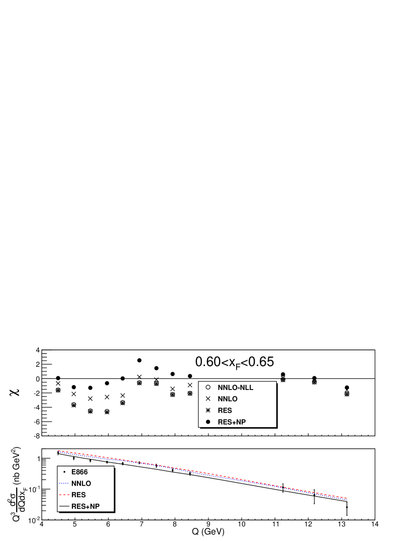
Figure 1: Different theoretical predictions compared to the E866 ($pp$) experimental data, with $0.60<x_{F}<0.65$. In the lower plot, the theoretical results have been multiplied by $1/N_{2}$.

Next, let us compare various theory calculations to the large $Q$ (around 100 GeV) DY data, taken by the CDF Collaboration at the Tevatron Run-2.

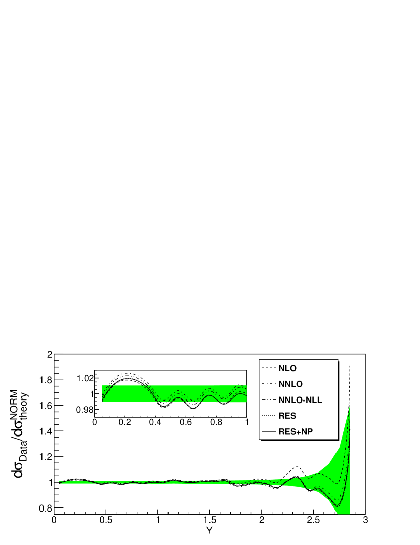
Figure 2: The ratio of CDF Run-2 DY data to various theoretical predictions (after being multiplied by $1/N_{3}$). The shaded area indicates the statistical error of the data.

As shown in Fig. 2, for $Y>2$, the NLO result becomes smaller than the data while the NNLO, RES and RES+NP calculations give similar results, though the RES+NP result gives the lowest $\chi^{2}$ for this set of data, cf. Table 2. We could also compare the total cross section of the DY pair produced at the Tevatron Run-2 and the LHC. The result of comparison is listed in Table 3.

$\sigma(p\bar{p}/pp\to l^{+}l^{-}+X)(\text{pb})$	NLO	NNLO	RES	RES+NP
Tevatron	240.7	242.0	248.0	247.98
LHC	2047.9	2036.8	2115.2	2115.3

Table 3: The total cross sections of the DY pair (with $66\/\text{GeV}<Q<116\/\text{GeV}$) produced at the Tevatron Run-2 and the LHC.

It shows that the results of RES and RES+NP are about the same, and differ from NNLO (and NLO) by about $2.5\%$ at the Tevatron and $3.7\%$ at the LHC. Hence, we conclude that the effect from the NP correction terms to the conventional threshold resummation formalism for large $Q$ values in high energy hadron collisions is not important.

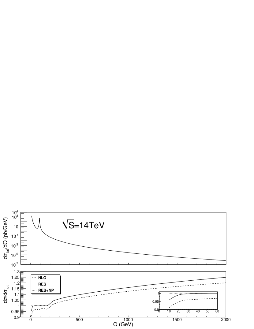
Figure 3: The differential cross section as a function of the invariant mass of the DY pair produced at the LHC.

Finally, we show in Fig. 3 the differential cross section as a function of the invariant mass of the DY pair produced at the LHC. In this figure, $d\sigma_{\text{SUM}}/dQ$ represents the differential cross section including the RES+NP result and the electroweak box diagram contribution, originated from the re-scattering of $W$ and $Z$ bosons in loop diagrams [25]. In order to study in detail the higher order correction to the shape of the $d\sigma/dQ$ distribution, we also plot the ratio of differential cross sections normalized by $d\sigma_{\text{SUM}}/dQ$. The label RES+NP indicates the ratio of $d\sigma_{\text{RES+NP}}/d\sigma_{\text{SUM}}$, etc. It is evident that the results of RES and RES+NP are almost the same except when the value of $Q$ is small, less than about 30 GeV.

5 Conclusion

In conclusion, we have investigated the NP effect in the threshold resummation calculations. From analyzing the asymptotic behavior of the conventional threshold resummation formalism (RES), we proposed the NP correction terms to be included in the improved threshold resummation formalism (RES+NP). They are subsequently determined by fitting to the DY data from E605, E866 ($pp$) and CDF Run-2 experiments. We found that to describe the low energy DY data with relatively small value of invariant mass, the NP effect cannot be ignored in threshold resummation calculation. In contrast, the minimal prescription threshold resummation formalism (RES) gives a similar prediction as RES+NP when the invariant mass of the DY pair is large. Though it remains to be seen how well the threshold resummation formalism could describe the top quark pair production rates at the Tevatron and the LHC [26], the type of NP effect discussed in this paper is not expected to be important. On the contrary, this effect will become relevant for describing the low invariant mass DY pairs produced at the Relativistic Heavy Ion Collider (RHIC) at the Brookhaven Laboratory.

References

• [1] E. Laenen, G. Oderda and G. Sterman, Phys. Lett.  B 438 (1998) 173 [arXiv:hep-ph/9806467].
• [2] S. Fanchiotti, B. A. Kniehl and A. Sirlin, Phys. Rev.  D 48 (1993) 307 [arXiv:hep-ph/9212285].
• [3] N. Kidonakis, Int. J. Mod. Phys.  A 15 (2000) 1245 [arXiv:hep-ph/9902484].
• [4] H. Contopanagos and G. Sterman, Nucl. Phys.  B 419 (1994) 77 [arXiv:hep-ph/9310313]; E. L. Berger and H. Contopanagos, Phys. Lett.  B 361 (1995) 115 [arXiv:hep-ph/9507363]; E. L. Berger and H. Contopanagos, Phys. Rev.  D 54 (1996) 3085 [arXiv:hep-ph/9603326]; E. L. Berger and H. Contopanagos, Phys. Rev.  D 57 (1998) 253 [arXiv:hep-ph/9706206].
• [5] S. Catani, M. L. Mangano, P. Nason and L. Trentadue, Nucl. Phys.  B 478 (1996) 273 [arXiv:hep-ph/9604351].
• [6] M. Bonvini, S. Forte and G. Ridolfi, Nucl. Phys.  B 808 (2009) 347 [arXiv:0807.3830 [hep-ph]].
• [7] T. Becher and M. Neubert, Phys. Rev. Lett. 97 (2006) 082001 [arXiv:hep-ph/0605050].
• [8] N. Kidonakis, E. Laenen, S. Moch and R. Vogt, Phys. Rev.  D 64 (2001) 114001 [arXiv:hep-ph/0105041].
• [9] G. Moreno et al., Phys. Rev.  D 43 (1991) 2815.
• [10] J. C. Webb, arXiv:hep-ex/0301031; J. C. Webb et al. [NuSea Collaboration], arXiv:hep-ex/0302019.
• [11] J. Han, A. Bodek, W. Sakumoto and Y. Chung, J. Phys. Conf. Ser.  110 (2008) 042009.
• [12] D. Choudhury, S. Majhi and V. Ravindran, JHEP 0601 (2006) 027 [arXiv:hep-ph/0509057].
• [13] A. Mukherjee and W. Vogelsang, Phys. Rev.  D 73 (2006) 074005 [arXiv:hep-ph/0601162].
• [14] P. Bolzoni, Phys. Lett.  B 643 (2006) 325 [arXiv:hep-ph/0609073].
• [15] J. C. Collins and D. E. Soper, Nucl. Phys.  B 194 (1982) 445.
• [16] N. Kidonakis, Int. J. Mod. Phys.  A 19 (2004) 1793 [arXiv:hep-ph/0303186].
• [17] C. Anastasiou, L. J. Dixon, K. Melnikov and F. Petriello, Phys. Rev. Lett.  91 (2003) 182002 [arXiv:hep-ph/0306192].
• [18] N. Kidonakis, JHEP 0505 (2005) 011 [arXiv:hep-ph/0412422].
• [19] E. Laenen, G. Sterman and W. Vogelsang, Phys. Rev.  D 63 (2001) 114018 [arXiv:hep-ph/0010080].
• [20] C. Amsler et al. [Particle Data Group], Phys. Lett.  B 667 (2008) 1.
• [21] P. M. Nadolsky et al., Phys. Rev.  D 78 (2008) 013004 [arXiv:0802.0007 [hep-ph]].
• [22] D. Stump et al., Phys. Rev.  D 65 (2001) 014012 [arXiv:hep-ph/0101051].
• [23] P. Mathews, V. Ravindran, K. Sridhar and W. L. van Neerven, Nucl. Phys.  B 713 (2005) 333 [arXiv:hep-ph/0411018].
• [24] K. Melnikov and F. Petriello, Phys. Rev.  D 74 (2006) 114017 [arXiv:hep-ph/0609070].
• [25] U. Baur, O. Brein, W. Hollik, C. Schappacher and D. Wackeroth, Phys. Rev.  D 65 (2002) 033007 [arXiv:hep-ph/0108274].
• [26] M. Czakon and A. Mitov, arXiv:0812.0353 [hep-ph].