A greedy algorithm for the identification of quantum systems.

Abstract

The control of quantum phenomena is a topic that has carried out many challenging problems. Among others, the Hamiltonian identification, i.e, the inverse problem associated with the unknown features of a quantum system is still an open issue. In this work, we present an algorithm that enables to design a set of selective laser fields that can be used, in a second stage, to identify unknown parameters of quantum systems.

1 Introduction

The possibility to use coherent light to manipulate molecular systems at the nanoscale has been demonstrated both theoretically [1] and experimentally [15]. Different types of methods have proven their relevancy for various settings, ranging from electron to large polyatomic molecules [2, 6, 8, 9, 13].
At the same time, the ability to generate a large amount of quantum dynamics data in a small time frame can also be used to extract from experiments the values of unknown parameters of quantum systems. The corresponding inverse problem, usually called Hamiltonian identification has recently been subject to significant developments through encouraging experimental results [4].
Various formulations in an optimization settings have been studied. Because of the nature of the available data, zero order methods were first tested, see e.g. the technique of map inversion [16]. The use of optimal control techniques was then introduced [3, 5].
Contrary to this last class of methods, we present in this work a methodology that enables to handle situations where the experimental measurements are provided only at a given time. Our approach is based on a precomputation that provides a family of selective laser fields. Roughly speaking, these laser fields are designed iteratively to highlight variations in the parameters that are subject to the identification. In a second stage, these fields and the experimental measurements are used to assemble a nonlinear system satisfied by the to-be-identified parameters.
The paper is organized as follows: the optimization framework and the assumptions we use are presented in Sec. 2. In Sec. 3, the structure of our algorithm is given. The procedures used in the two parts of this algorithm are described in Sec. 4 and Sec. 5. The identification step is explained in Sec. 6. Details about practical implementation and some numerical results are given Sec. 7. We conclude with some remarks in Sec. 8.
Throughout this paper, $\Omega$ is a spacial domain in $\mathbb{R}^{d}$, $d=1,2,3$, $L^{2}$ denotes the space of complex valued square integrable functions over $\Omega$, and $\langle.,.\rangle$ the usual Hermitian product associated to $L^{2}$. The following standard convention is used:

$$\langle a|O|b\rangle:=\langle a,O(b)\rangle,\ a\in L^{2},\ b\in L^{2},\ O\in{\cal L}(L^{2};L^{2})$$

the set of all linear operator from $L^{2}$ into $L^{2}$. Finally, we use $\Re(z),\Im(z)$ to denote respectively the real and the imaginary part of a complex number $z$.

2 The identification problem

We first introduce the model and the framework used in this paper.

2.1 Control of the Schrödinger Equation

Consider a quantum system $\psi\in H^{1}$, with norm $\|\psi\|_{L^{2}}=1$, evolving according to the Schrödinger equation

$$\left\{\begin{array}[]{ccl}i\dot{\psi}&=&[H_{0}+V+\varepsilon(t)\mu]\psi\\ \psi(0)&=&\psi_{0},\end{array}\right.$$ (1)

where $H_{0}$ is the kinetic energy operator, $V\in{\cal L}(L^{2};L^{2})$ the potential operator and $\mu\in{\cal L}(L^{2};L^{2})$ the dipole moment operator coupling the system to a time-dependent external laser field $\varepsilon(t)$. In this context, $\varepsilon$ reads as a control since it can be chosen by the experimenter.

In the settings we consider here, we assume that the internal Hamiltonian $H=H_{0}+V$ is known so that the goal is to identify the dipole moment operator $\mu$. The generalization to the identification of $V$ should not give rise to any particular problem and is left to a future contribution.

The basic hypothesis made on $\mu$ is that it belongs to (or actually can be conveniently approximated by) a finite dimensional space spanned by some basis set $\mathcal{B}_{\mu}=(\mu_{\ell})_{\ell=1,\dots,L}$.

2.2 Experimental measurements and controllability

In order to perform the identification, we assume that given a time $T$ and a laser field $\varepsilon\in L^{2}(0,T)$, the experimenter can measure, for some fixed state $\psi_{1}\in L^{2}$, with norm $\|\psi_{1}\|_{L^{2}}=1$, the value $\varphi(\mu,\varepsilon):=\langle\psi_{1},\psi(T)\rangle$.
Note that all what follows still holds when considering several measurements a time $T$, i.e., in the case where a set of measurement $\left(\langle\psi_{\ell},\psi(T)\rangle\right)_{\ell=1\dots,p}$, with $p>1$, is known.
Finally, we assume that the system under consideration is wavefunction controllable, i.e., that $\varepsilon\in L^{2}(0,T)\mapsto\psi(T)$ is surjective.

2.3 Formulation of problem

Our identification method is based on a particular formulation of the identification problem that we now briefly introduce.
Denote by $\mu^{\star}$ the actual dipole moment operator of a given system. The solution $\mu=\mu^{\star}$ of our problem also solves the minimization problem:

$$\inf_{\mu\in{\cal L}(L^{2};L^{2})}\sup_{\varepsilon\in L^{2}(0,T)}|\varphi(\mu,\varepsilon)-\varphi(\mu^{\star},\varepsilon)|^{2}.$$ (2)

This settings highlights the fact that as long as $\mu\neq\mu^{\star}$, a selective laser field should be designed so that the difference between $\mu$ and $\mu^{\star}$ is discerned through the measurement $\varphi(\mu,\varepsilon)$.

3 Structure of the algorithm

Our algorithm consists in designing, through a finite iterative procedure, a set of selective laser fields. We start with the general structure of our algorithm. Details about its steps are given in the next sections.

3.1 The selective laser fields computation greedy algorithm

Starting from the basis set $\mathcal{B}_{\mu}=(\mu_{\ell})_{\ell=1,\dots,L}$, the algorithm builds up iteratively a set of $L$ selective laser fields as follows.

Algorithm 1

(Selective laser fields computation greedy algorithm) Let us define $\varepsilon^{1}$ a laser field that solves the problem:

$$\sup_{\varepsilon\in L^{2}(0,T)}|\varphi(\mu_{1},\varepsilon)|^{2}.$$

Suppose now that at the step $k$, with $1<k\leq L$, a laser field $\varepsilon^{k-1}$ is given. The computation of $\varepsilon^{k}$ is performed according to the two following sub-steps:

1. Fitting step : Find $(\alpha^{k}_{j})_{j=1,\dots,k-1}$ that solves the problem:

   $$\left\{\begin{array}[]{ccl}\varphi(\sum_{j=1}^{k-1}\alpha^{k}_{j}\mu^{j},\varepsilon^{1})&=&\varphi(\mu^{k},\varepsilon^{1})\\ &\vdots&\\ \varphi(\sum_{j=1}^{k-1}\alpha^{k}_{j}\mu^{j},\varepsilon^{m})&=&\varphi(\mu^{k},\varepsilon^{m})\\ &\vdots&\\ \varphi(\sum_{j=1}^{k-1}\alpha^{k}_{j}\mu^{j},\varepsilon^{k-1})&=&\varphi(\mu^{k},\varepsilon^{k-1}),\end{array}\right.$$ (3)

   in the minimum mean square error sense.

2. Discriminatory step : Find $\varepsilon^{k}$ that solves the problem:

   $$\varepsilon^{k}=\hbox{argmax}_{\varepsilon\in L^{2}(0,T)}|\varphi(\mu^{k},\varepsilon)-\varphi(\sum_{j=1}^{k-1}\alpha^{k}_{j}\mu^{j},\varepsilon)|^{2}.$$

The initialization of the algorithm is somehow arbitrary, the only requirement is that $\varepsilon^{1}$ has a link with the type of measurement. In our case, we decide to maximize it.

Remark 1

Note that, in opposition to usual approaches (see e.g. [5, 3]), our method plays the role of a precomputation step since the actual measurements $\varphi(\mu^{\star},\varepsilon)$ are not required at this stage.

3.2 Intuitive interpretation of the algorithm

In the first sub-step of an iteration of Algorithm 1, one looks for a defect of selectivity of the current laser fields $\varepsilon^{1},\dots,\varepsilon^{k-1}$: in the case the minimum reaches zero, two distinct dipole moment operators give rise to two identical measurements when exited with the laser fields $\varepsilon^{1},\dots,\varepsilon^{k-1}$. On the contrary, the second sub-step aims at computing a laser field that compensates this defect. These two sub-steps corresponds respectively to the minimization part and to the maximization part of the formulation (2).

Remark 2

Even if no hierarchy is assumed in the basis $\mathcal{B}_{\mu}$, this algorithm should be viewed as a first step towards future works that handle infinite dimensional systems. In such a framework, the sum $\sum_{j=1}^{k-1}\alpha^{k}_{j}\mu^{j}$ would read as an asymptotic expansion of the dipole moment operator.

This algorithm belongs to the class of greedy algorithms, since it follows the problem-solving’s heuristic of making the locally optimal choice (in the second sub-step) at each stage with the hope of finding the global optimum that solves (2).

4 Fitting step

Let us first focus on the first sub-step of the algorithm. Consider an integer $k$ such that $1<k\leq L$ and denote by $K^{k}$ the functional (defined on $\mathbb{R}^{k-1}$):

$$K^{k}(\alpha)=\sum_{m=1}^{k-1}|\varphi(\mu^{k},\varepsilon^{m})-\varphi(\sum_{j=1}^{k-1}\alpha_{j}\mu^{j},\varepsilon^{m})|^{2}.$$

During this sub-step, one has to find the minimum of the cost functional $K^{k}$. To do this, a standard global minimization algorithm applied to this minimum mean square error associated problem.
Note that, for small values of $L$, the gradient of the functional $K^{k}$ can be computed thanks to the formula:

$\nabla K^{k}(\alpha).\delta\alpha=$

$$\sum_{m=1}^{k-1}2\Re\left(\langle\psi_{\varepsilon^{m}}^{\alpha}(T)-\psi_{\varepsilon^{m}}^{k}(T),\psi_{1}\rangle\langle\delta\psi_{\varepsilon^{m}}^{\alpha}(T),\psi_{1}\rangle\right),$$

where $\psi_{\varepsilon^{m}}^{\alpha}$ and $\psi_{\varepsilon^{m}}^{k}$ are the solutions of Eq. (1) with $\varepsilon=\varepsilon^{m}$ as laser field, and $\mu=\sum_{j=1}^{k-1}\alpha_{j}\mu^{j}$ and $\mu=\mu^{k}$ respectively as dipole moment operator. The variation $\delta\psi^{\alpha}$ is computed thanks to:

$$\left\{\begin{array}[]{ccl}i\delta\dot{\psi}_{\varepsilon^{m}}^{\alpha}&=&\varepsilon^{k-1}\left(\sum_{j=1}^{k-1}\alpha_{j}\mu^{j}\right)\delta\psi_{\varepsilon^{m}}^{\alpha}\\ &&+[H_{0}+V+\varepsilon^{k-1}(t)\left(\sum_{j=1}^{k-1}\delta\alpha_{j}\mu^{j}\right)]\psi_{\varepsilon^{m}}^{\alpha}\\ \delta\psi_{\varepsilon^{m}}^{\alpha}(0)&=&0.\end{array}\right.$$

In this way the computation of the components of $\nabla K^{k}(\alpha)$ can be parallelized to make the use of gradient methods feasible.

5 Discriminatory step

To achieve the second sub-step of Algorithm 1, we adapt an efficient strategy usually used in in quantum control. This strategy has given rise to a large class of algorithms often called ”monotonic schemes”. For a general presentation of these algorithms, we refer to [11].

5.1 Improvement of the selectivity of a given laser field

Let us present in more details how this strategy applies in our case. Note first that, given a laser field $\varepsilon\in L^{2}(0,T)$, and two dipole moment operators $\widetilde{\mu}$ and $\widehat{\mu}$, one has:

$$|\varphi(\widetilde{\mu},\varepsilon)-\varphi(\widehat{\mu},\varepsilon)|^{2}=\langle\widetilde{\psi}(T)-\widehat{\psi}(T)|O_{\psi_{1}}|\widetilde{\psi}(T)-\widehat{\psi}(T)\rangle,$$

where $O_{\psi_{1}}=\psi_{1}.\psi_{1}^{T}$, $\widetilde{\psi}$ and $\widehat{\psi}$ are the solutions of Eq. (1) with respectively $\mu=\widetilde{\mu}$ and $\mu=\widehat{\mu}$ as dipole moment operator.

In order to compare the selectivity of $\varepsilon$ and $\varepsilon^{\prime}$, we introduce the functional:

$$J(\varepsilon)=\langle\widetilde{\psi}(T)-\widehat{\psi}(T)|O_{\psi_{1}}|\widetilde{\psi}(T)-\widehat{\psi}(T)\rangle-\beta\int_{0}^{T}\varepsilon^{2}(t)dt,$$

which has to be maximized. For sake of simplicity, we omit the dependence of $J$ with $\widetilde{\mu}$ and $\widehat{\mu}$ in the notations.
The additional term $\beta\int_{0}^{T}\varepsilon^{2}(t)dt$, is introduced for two complementary reasons: first, as it penalizes the $L^{2}$-norm of the laser field, it enables to obtain feasible laser fields and secondly, it improves the convergence of Algorithm 2 below.
Consider now another laser field $\varepsilon^{\prime}\in L^{2}(0,T)$, and denote by $\widetilde{\psi}^{\prime}$ and $\widehat{\psi}^{\prime}$ the corresponding solutions of Eq. (1) with $\mu=\widetilde{\mu}$ and $\mu=\widehat{\mu}$ respectively. We introduce the two adjoints states defined by:

$$\left\{\begin{array}[]{ccl}i\dot{\widetilde{\chi}}&=&[H_{0}+V+\varepsilon(t)\widetilde{\mu}]\widetilde{\chi}\\ \widetilde{\chi}(T)&=&O_{\psi_{1}}\left(\widetilde{\psi}(T)-\widehat{\psi}(T)\right),\end{array}\right.$$ (4)

and

$$\left\{\begin{array}[]{ccl}i\dot{\widehat{\chi}}&=&[H_{0}+V+\varepsilon(t)\widehat{\mu}]\widehat{\chi}\\ \widehat{\chi}(T)&=&O_{\psi_{1}}\left(\widetilde{\psi}(T)-\widehat{\psi}(T)\right).\end{array}\right.$$ (5)

One has:

$$J(\varepsilon^{\prime})-J(\varepsilon)=\langle\delta\psi^{\prime}(T)-\delta\psi(T)|O_{\psi_{1}}|\delta\psi^{\prime}(T)-\delta\psi(T)\rangle$$

$$+2\Re\langle\delta\psi^{\prime}(T)-\delta\psi(T),\widetilde{\chi}(T)-\widehat{\chi}(T)\rangle$$

$$-\beta\int_{0}^{T}\varepsilon^{\prime 2}(t)-\varepsilon^{2}(t)dt$$

$$=\langle\delta\psi^{\prime}(T)-\delta\psi(T)|O_{\psi_{1}}|\delta\psi^{\prime}(T)-\delta\psi(T)\rangle$$

$$+\int_{0}^{T}\left(\varepsilon^{\prime}(t)-\varepsilon(t)\right)$$

$$\left(2\Im\langle\widetilde{\chi}(t)|\widetilde{\mu}|\widetilde{\psi}^{\prime}(t)\rangle\!-\!2\Im\langle\widehat{\chi}(t)|\widehat{\mu}|\widehat{\psi}^{\prime}(t)\rangle\!-\!\beta\left(\varepsilon^{\prime}(t)\!+\!\varepsilon(t)\right)\right)dt,$$

(6)

where we denote $\delta\psi^{\prime}(T)=\widetilde{\psi}^{\prime}(T)-\widehat{\psi}^{\prime}(T)$ and $\delta\psi(T)=\widetilde{\psi}(T)-\widehat{\psi}(T)$. Identity (6) gives a criterion to guarantee that $\varepsilon^{\prime}$ is more selective than $\varepsilon$. Indeed, suppose that $\varepsilon^{\prime}$ satisfies for all $t\in[0,T]$ the condition:

$$\left(\varepsilon^{\prime}(t)-\varepsilon(t)\right)\left(2\Im\langle\widetilde{\chi}(t)|\widetilde{\mu}|\widetilde{\psi}^{\prime}(t)\rangle-2\Im\langle\widehat{\chi}(t)|\widehat{\mu}|\widehat{\psi}^{\prime}(t)\rangle\right.$$

$$\left.\phantom{\Im\langle\widetilde{\chi}(t)|\widetilde{\mu}|\widetilde{\psi}^{\prime}(t)\rangle}-\beta(\varepsilon^{\prime}(t)+\varepsilon(t))\right)\geq 0,$$ (7)

then $J(\varepsilon^{\prime})\geq J(\varepsilon)$.
Various ways to ensure that (7) holds. For example [14], one can define $\varepsilon^{\prime}$ at each time $t$ as the solution of the equation:

$$\varepsilon^{\prime}(t)-\varepsilon(t)=\frac{\theta}{\beta}\left(2\Im\langle\widetilde{\chi}(t)|\widetilde{\mu}|\widetilde{\psi}^{\prime}(t)\rangle-2\Im\langle\widehat{\chi}(t)|\widehat{\mu}|\widehat{\psi}^{\prime}(t)\rangle\right.$$

$$\left.\phantom{\Im\langle\widetilde{\chi}(t)|\widetilde{\mu}|\widetilde{\psi}^{\prime}(t)\rangle}-\beta\left(\varepsilon^{\prime}(t)+\varepsilon(t)\right)\right),$$

(8)

where $\theta$ is a given strictly positive number. In this case, one has:

$$J(\varepsilon^{\prime})-J(\varepsilon) \!\!=\!\! \langle\delta\psi^{\prime}(T)-\delta\psi(T)|O_{\psi_{1}}|\delta\psi^{\prime}(T)-\delta\psi(T)\rangle$$

$$+\frac{\beta}{\theta}\int_{0}^{T}\left(\varepsilon^{\prime}(t)-\varepsilon(t)\right)^{2}dt\geq 0,$$

which is the desired conclusion. In Sec. 7.1, we present an alternative that can be obtained in a time discretized settings.

5.2 Discriminatory sub-algorithm

We derive form the previous considerations the following iterative procedure to define a laser field $\varepsilon^{k}$ that maximizes $J(\varepsilon)$:

Algorithm 2

(Discriminatory sub-algorithm) Let $Tol$ be a positive number. Consider an initial guess $\varepsilon^{k}_{0}$ and compute the corresponding solutions of Eq. (1) with $\widetilde{\mu}$ and $\widehat{\mu}$, say $\widetilde{\psi}_{0}$ and $\widehat{\psi}_{0}$. Set $err=2.Tol$.
While $err>Tol$, do:

1. Use Eqs. (4–5) with $\varepsilon=\varepsilon^{k}_{\ell}$, $\widetilde{\psi}=\widetilde{\psi}_{\ell}$ and $\widehat{\psi}=\widehat{\psi}_{\ell}$, to compute $\widetilde{\chi}_{\ell}$ and $\widehat{\chi}_{\ell}$, respectively.

2. Compute simultaneously the laser field $\varepsilon^{k}_{\ell+1}$ and the states $\widetilde{\psi}_{\ell+1}$ and $\widehat{\psi}_{\ell+1}$ the solutions of coupled system composed of Eq. (8) with $\widetilde{\chi}=\widetilde{\chi}_{\ell}$, $\widehat{\chi}=\widehat{\chi}_{\ell}$ and Eq. (1) with $\mu=\widetilde{\mu}$ and $\mu=\widehat{\mu}$ respectively.

3. $\ell\leftarrow\ell+1$, $err=|\varepsilon^{k}_{\ell+1}-\varepsilon^{k}_{\ell}|$.

In [7], one shows that Eq. (8) has a solution and presents some efficient numerical nonlinear solvers to compute it.

6 Identification procedure

Once the $L$ selective fields $\varepsilon^{1},...,\varepsilon^{L}$ have been computed, one can use them experimentally to obtain the corresponding measurements $\varphi(\mu^{\star},\varepsilon^{1}),...,\varphi(\mu^{\star},\varepsilon^{L})$.
The identification procedure consists then in finding the linear combination $(\alpha^{1},...,\alpha^{L})$ that solves the following nonlinear system:

$$\left\{\begin{array}[]{ccl}\varphi(\sum_{j=1}^{L}\alpha_{j}\mu^{j},\varepsilon^{1})&=&\varphi(\mu^{\star},\varepsilon^{1})\\ &\vdots&\\ \varphi(\sum_{j=1}^{L}\alpha_{j}\mu^{j},\varepsilon^{k})&=&\varphi(\mu^{\star},\varepsilon^{k})\\ &\vdots&\\ \varphi(\sum_{j=1}^{L}\alpha_{j}\mu^{j},\varepsilon^{L})&=&\varphi(\mu^{\star},\varepsilon^{L}).\end{array}\right.$$ (9)

in the mean square sense. In this view, the standard global optimization procedure used for the first sub-step of algorithm can be applied to the associated problem.
Note that, in a finite-dimensional settings, the existence of a solution is guaranteed.

7 Numerical implementation and results

We give here details about the practical implementation of Algorithm 1, and show its efficiency on an example.

7.1 Numerical solvers

In order to solve numerically Eq. (1), we use the second order Strang operator splitting [12]. Given $M>0$, a time step $\Delta t$ such that $M.\Delta t=T$ and an approximation $\psi_{j}$ of $\psi(j.\Delta t)$ with $j<M$, this method leads in our case to the following iteration:

$$\psi_{j+1}=e^{iH\frac{\Delta t}{2}}e^{i\varepsilon_{j}\mu\Delta t}e^{iH\frac{\Delta t}{2}}\psi_{j}.$$ (10)

In the second sub-step of Algorithm 1, Discriminatory sub-algorithm 2 is adapted to this discrete settings. In this way, we consider the time-discretized version of the cost functional $J$:

$$J_{\Delta t}(\varepsilon)=\langle\widetilde{\psi}_{M}-\widehat{\psi}_{M}|O_{\psi_{1}}|\widetilde{\psi}_{M}-\widehat{\psi}_{M}\rangle-\beta\Delta t\sum_{j=0}^{M-1}\varepsilon_{j}^{2},$$

where $\varepsilon\in\mathbb{R}^{M-1}$. Fix now two discrete laser fields $\varepsilon$ and $\varepsilon^{\prime}$, one can then repeat the computation done in Sec. 5.1 to obtain:

$$J_{\Delta t}(\varepsilon^{\prime})-J_{\Delta t}(\varepsilon)=\langle\delta\psi^{\prime}_{M}-\delta\psi_{M}|O_{\psi_{1}}|\delta\psi^{\prime}_{M}-\delta\psi_{M}\rangle$$

$$+\Delta t\sum_{j=0}^{M-1}\left(\varepsilon^{\prime}_{j}-\varepsilon_{j}\right)$$

$$\left(2\Im\langle\widetilde{\chi}_{j}|\widetilde{\mu}_{\Delta t}(\varepsilon^{\prime}_{j},\varepsilon_{j})|\widetilde{\psi}^{\prime}_{j}\rangle-2\Im\langle\widehat{\chi}_{j}|\widehat{\mu}_{\Delta t}(\varepsilon^{\prime}_{j},\varepsilon_{j})|\widehat{\psi}^{\prime}_{j}\rangle\right.$$

$$\left.\phantom{2\Im\langle\widetilde{\chi}_{j}|\widehat{\mu}_{\Delta t}(\varepsilon^{\prime}_{j},\varepsilon_{j})|\widehat{\psi}^{\prime}_{j}\rangle}-\beta\left(\varepsilon^{\prime}_{j}+\varepsilon_{j}\right)\right),$$ (11)

where the vectors $\widetilde{\chi}$, $\widehat{\chi}$, $\widetilde{\psi}^{\prime}$ and $\widehat{\psi}^{\prime}$ are computed using the iteration (10) with $\mu=\widetilde{\mu}_{\Delta t}(\varepsilon^{\prime}_{j},\varepsilon_{j})$ and $\mu=\widehat{\mu}_{\Delta t}(\varepsilon^{\prime}_{j},\varepsilon_{j})$. These matrices are the approximations of $\widetilde{\mu}$ and $\widehat{\mu}$ respectively defined by:

$$\begin{array}[]{ccl}\widetilde{\mu}_{\Delta t}(\varepsilon^{\prime}_{j},\varepsilon_{j})&=&e^{-iH\frac{\Delta t}{2}}\dfrac{e^{i\varepsilon^{\prime}_{j}\widetilde{\mu}\Delta t}-e^{i\varepsilon_{j}\widetilde{\mu}\Delta t}}{i\Delta t(\varepsilon^{\prime}_{j}-\varepsilon_{j})}e^{iH\frac{\Delta t}{2}}\\ \widehat{\mu}_{\Delta t}(\varepsilon^{\prime}_{j},\varepsilon_{j})&=&e^{-iH\frac{\Delta t}{2}}\dfrac{e^{i\varepsilon^{\prime}_{j}\widehat{\mu}\Delta t}-e^{i\varepsilon_{j}\widehat{\mu}\Delta t}}{i\Delta t(\varepsilon^{\prime}_{j}-\varepsilon_{j})}e^{iH\frac{\Delta t}{2}}.\end{array}$$

For the sake of simplicity, instead of solving the discrete version of Eq. (8), we compute $\varepsilon^{\prime}_{j}$ using one step of a Newton optimization method applied to its corresponding term in the sum of Eq. (11). This strategy, and the one corresponding to Eq. (8) are presented in more details in [7]. Their convergence are proven in [10].

7.2 Numerical test

7.2.1 Settings

To illustrate the ability of our approach, we consider a simple finite dimensional settings where $H_{0},\ V$ and $\mu$ are $3\times 3$ Hermitian matrices with entries in $\mathbb{C}$ and $\psi(t)\in\mathbb{C}^{3}$. The internal Hamiltonian we consider is:

$$H=10^{-2}\left(\begin{array}[]{ccc}1&0&0\\ 0&2&0\\ 0&0&4\end{array}\right).$$

Since Eq. (1) with such an internal Hamiltonian is generically controllable, we choose to define the basis $\mathcal{B}_{\mu}$ randomly so that the systems handled by our algorithm are almost surely controllable.
In order to work in a general framework, we chose $\mu^{\star}$ also randomly. In our example, we consider:

$$\mu^{\star}=\left(\begin{array}[]{ccc}2.4154&1.9335&1.5822\\ 1.9335&1.4366&1.5991\\ 1.5822&1.5991&1.9843\end{array}\right).$$

The states $\psi_{0}$ and $\psi_{1}$ are

$$\psi_{0}=\left(\begin{array}[]{c}1\\ 0\\ 0\end{array}\right),\quad\psi_{1}=\left(\begin{array}[]{c}0\\ 0\\ 1\end{array}\right).$$

We choose $T=4000\pi$, which corresponds to $20$ periods of the transition associated to the smallest frequency of the system.

7.2.2 Algorithm parameters

The minimum mean square error problems (3)-(9) are solved by standard pseudo-Newton solvers. In order to make a global search, we repeat the minimization 10 times with random initialization. The parameter $\beta$ is adapted to make Algorithm 2 converge. In our case $\beta=10^{-2}$.

7.2.3 Numerical results

The precomputation is achieved by our algorithm in approximately 80 min CPU. The dipole moment operator is regained with a relative error

$$\frac{\|\mu^{\star}-\mu\|_{2}}{\|\mu^{\star}\|_{2}}\approx 9.8960e-04,$$

in approximately 10 min CPU. The selective fields that have been obtained are depicted in Fig. 1.

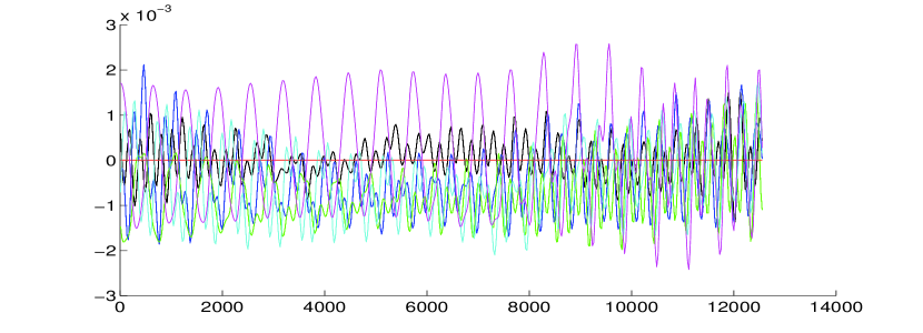
Figure 1: Selective laser fields obtained by Algorithm 2.

8 Concluding remarks

The Selective laser fields computation greedy algorithm presented in this paper shows a good efficiency in a general settings. However, there is some room for improvement of our strategy. First, the choice of the basis $\mathcal{B}_{\mu}$ could be improved, e.g. through an iterative procedure. Secondly, the experimental measurements could be used during the computation of the selective fields in order to design an online procedure. Lastly, some work has to be done to design a more specific approach to treat the first sub-step of the algorithm. The identification procedure presented in Sec. 6 would also certainly take advantage of such a study.

9 ACKNOWLEDGMENTS

The problem of identification in this context was raised during discussions with H. Rabitz from Princeton University and G. Turinici from Dauphine University, we thank them for helpful inputs. This work was supported by the french A.N.R, “Programme blanc C-Quid” and PICS CNRS-NSF collaboration between the Department of Chemistry, Princeton University, and University Paris Dauphine.

References

• [1] K. Beauchard, Local controllability of a 1D Schrödinger equation , J. Math. Pures et Appl., vol. 84, 2005, pp 851-956.
• [2] C. Le Bris, Y. Maday, and G. Turinici. Towards efficient numerical approaches for quantum control. In Quantum Control: mathematical and numerical challenges, A. Bandrauk, M.C. Delfour, and C. Le Bris, editors, CRM Proc. Lect. Notes Ser., pp 127–142, AMS Publications, Providence, R.I., 2003.
• [3] C. Le Bris, M. Mirrahimi, H. Rabitz and G. Turinici, Hamiltonian Identification for Quantum Systems: Well-posedness and Numerical Approaches, ESAIM: Control, Optimization and Calculus of Variations, vol. 13 (2), 2007, pp 378-395.
• [4] J.M. Geremia and H. Rabitz, Optimal identification of Hamiltonian information by closed-loop laser control of quantum systems, Physical review letters, vol. 89 (26), 2002, pp. 263902.1-263902.4.
• [5] J.M. Geremia and H. Rabitz, Optimal Hamiltonian identification: The synthesis of quantum optimal control and quantum inversion, J. Chem. Phys., vol. 118 (12), 2003, pp. 5369–5382.
• [6] R.J. Levis, G. Menkir and H. Rabitz, Selective bond dissociation and rearrangement with optimally tailored, strong-field laser pulses, Science,vol. 292, 2001, pp 709–712.
• [7] Y. Maday, J. Salomon, G. Turinici, Monotonic time-discretized schemes in quantum control, Numerische Mathematik, vol. 103, 2006, pp 323-338.
• [8] S. Rice and M. Zhao, Optimal Control of Quatum Dynamics. Wiley (2000).
• [9] N. Shenvi, J.M. Geremia and H. Rabitz, Nonlinear kinetic parameter identification through map inversion, J. Phys. Chem. A, vol. 106, 2002, pp 12315–12323.
• [10] J. Salomon, Convergence of the time-discretized monotonic schemes, M2AN, vol. 41 (1), 2007, pp. 77–93.
• [11] J. Salomon, G. Turinici, A monotonic method for solving nonlinear optimal control problems, Preprint HAL : hal-00335297, 2008,
http://hal.archives-ouvertes.fr/docs/00/33/52/
97/PDF/Salomon_Turinici.pdf
• [12] G. Strang, On the construction and comparison of difference schemes, SIAM J. Numer. Anal., 5, 1968, pp. 506–517.
• [13] M. Tadi and H. Rabitz, Explicit method for parameter identification, J. Guid. Control Dyn., vol. 20, 1997, pp 486–491.
• [14] D. Tannor, V. Kazakov, and V. Orlov. Control of photochemical branching : Novel procedures fornding optimal pulses and global upper bounds. In Broeckhove J. and Lathouwers L., editors, Time Dependent Quantum Molecular Dynamics, pp 347–360.
• [15] T. Weinacht, J. Ahn and P. Bucksbaum, Controlling the shape of a quantum wavefunction, Nature, vol. 397, 1999, pp 233–235.
• [16] N. Shenvi, J.M. Geremia and H. Rabitz, Nonlinear kinetic parameter identification through map inversion, J. Phys. Chem., A 106, 2002, pp 12315–12323.