Decoherence-free quantum dynamics in circuit QED system

Abstract

We study decoherence in a circuit QED system consisting of a charge qubit and two superconducting transmission line resonators (TLRs). We show that in the dispersive regime of the circuit QED system one TLR can be used as an auxiliary subsystem to realize decoherence-free quantum dynamics of the bipartite target system consisting of the charge qubit and the other TLR conditioned on the auxiliary TLR initially being a proper number state. Our study gives new insight into control and manipulation of decoherence in quantum systems.

I Introduction

Decoherence remains a major obstacle to experimental realizations of quantum computation and communication 1 ; 2 . As is well known, no system can be completely isolated from its environment. Interactions between the system and the environment create decoherence. There are some interesting methods to bypass decoherence in quantum information processing. One of them is to encode quantum information into decoherence-free subspaces and subsystems (DFSs) 3 ; 4 ; 5 ; 6 ; 7 ; 8 ; 9 . Under certain conditions, a subspace of a physical system is decoupled from its environment such that the dynamics within this subspace is purely unitary. The DFS is a set of all states which is not Experimental realizations of DFSs have been achieved in photon systems 10 ; 11 ; 12 ; 13 , nuclear spin systems 14 ; 15 ; 16 , and trapped-ion systems 17 ; 18 .

Advances in circuit QED [19-42] opened new prospects in nonclassical state generation and quantum information processing in the microwave regime. In the circuit QED, superconducting circuits are made to act like artificial atoms and a one-dimensional superconducting transmission line resonator (TLR) forms a microwave cavity. Unlike natural atoms, the properties of artificial atoms made from circuits can be designed to taste, and even manipulated in-situ. Because the qubit contains many atoms, the effective dipole moment can be much larger than an ordinary alkali atom and a Rydberg atom. This allows circuits to couple much more strongly to the cavity. This large coherent coupling allows circuits to achieve strong coupling even in the presence of the larger decoherence present in the solid state environment, then one can observe the quantum interactions of matter with single photons. Hence, circuit QED can explore new regimes of cavity QED. Recently, the circuit QED systems have successfully demonstrated strong coupling between a single microwave photon and a qubit 20 , the implementation of a single microwave-photon source in all solid-state system 21 , as well as single artificial-atom lasing 22 and interaction between two artificial atoms 23 ; 24 . More recently, the Lamb shift, two-photon Jaynes-Cummings model and controlled symmetry breaking 25 have also been observed experimentally in circuit-QED systems 26 ; 27 . These give rise to strong experimental supports for on-chip quantum optics and quantum information processing.

In this paper, we are concerned with decoherence in a circuit QED system which includes one SQUID-type charge qubit acting as an artificial atom and two superconducting TLRs. We show that in the dispersive regime of the circuit QED system one TLR can be used as an auxiliary subsystem to realize decoherence-free quantum dynamics of the bipartite target system consisting of the charge qubit and the other TLR. The paper is organized as follows. In Sec. II, we propose the physical model under our consideration and present its analytical solution in the dispersive regime. In Sec. II, we investigate DFS of the circuit-QED system. We show how to realize decoherence-free quantum dynamics of the bipartite target system. We shall conclude the paper with discussions and remarks in the last section.

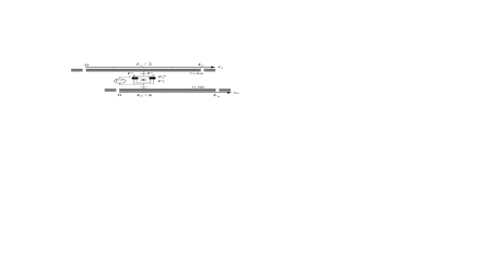
Figure 1: Schematic setup for the proposed circuit-QED system. The SQUID-based charge qubit is coupled with two TLRs, TLRA and TLRB, of lengths $L_{a}$ and $L_{b}$, respectively. The SQUID is placed at the position of the antinode of the quantized voltage of TLRA (i.e., $L_{a}/2$) and the antinode of the quantized current of TLRB (i.e., $L_{b}/4$), respectively.

II Physical model

Let us illustrate our idea firstly. As shown in Fig.1, we consider a circuit-QED system in which an SQUID-type charge qubit is coupled to two transmission line resonators, TLRA and TLRB, of lengths $L_{a}$ and $L_{b}$, respectively. The qubit is placed at the position of the antinode of the quantized voltage of TLRA (i.e., $x_{a}=L_{a}/2$) and the antinode of the quantized current of TLRB (i.e., $x_{b}=L_{b}/4$), respectively. It can be controlled by the gate voltage, which contains the dc part $V_{g}^{dc}$ and the quantum part $V_{a}$ generated by the TLRA, and the biasing flux $\Phi$, which contains the classical part $\Phi_{e}$ and the quantized part $\Phi_{b}$ generated by the TLRB threading the SQUID.

In terms of the annihilation operator $a(b)$ and creation operator $a^{{\dagger}}(b^{{\dagger}})$ of TLRA (TLRB), the Hamiltonian for this system reads as 19 ; 20

$$H=\hbar\omega_{a}a^{{\dagger}}a+\hbar\omega_{b}b^{{\dagger}}b+2E_{C}(2n_{g}-1)\sigma_{z}-E_{J}\sigma_{x},$$ (1)

where $\omega_{a}$ and $\omega_{b}$ are the microwave frequencies of TLRA and TLRB, respectively. The last two terms represent the Hamiltonian of the charge qubit. Here $\sigma_{z}=|1\rangle\langle 1|-|0\rangle\langle 0|$ and $\sigma_{x}=|1\rangle\langle 0|+|0\rangle\langle 1|$ with $0(1)$ the number of Cooper pairs on the superconducting island. $E_{C}=e^{2}/2C_{\Sigma}$ is the charging energy with $C_{\Sigma}$ being the total box capacitance. $n_{g}$ is the gate charge number and $E_{J}$ is the Josephson coupling energy given by

$$n_{g}=\frac{C_{g}V_{g}^{dc}+C_{a}V_{a}}{2e},\;\;\;\;\;\;\;E_{J}=E_{J}^{m}\cos\left(\pi\frac{\Phi}{\Phi_{0}}\right),$$ (2)

where $C_{g}$ and $C_{a}$ represent the gate capacitance and the coupling capacitance between TLRA and the charge qubit. $V_{g}^{dc}$ and $V_{a}$ are the dc gate voltage and the quantum gate voltage generated by TLRA, respectively. $E_{J}^{m}$ is the maximum Josephson coupling energy and $\Phi_{0}$ is the flux quanta. The total magnetic flux $\Phi$ threading the dc-SQUID is a sum of two parts $\Phi=\Phi_{b}+\Phi_{e}$ with $\Phi_{e}$ being the external classical magnetic flux and $\Phi_{b}$ the quantized magnetic flux generated by the quantized current in TLRB.

The quantum gate voltage and the quantized magnetic flux associated with TLRA and TLRB can be expressed in terms of the annihilation and creation operators of the microwave fields in TLRA and TLRB as

$$V_{a} = -\sqrt{\frac{\hbar\omega_{a}}{L_{a}c}}(a+a^{{\dagger}}),$$

$$\Phi_{b} = \frac{\mu_{0}S}{2\pi d}\sqrt{\frac{\hbar\omega_{b}}{L_{b}l}}(b+b^{{\dagger}}),$$ (3)

where $c$ and $l$ are the capacitance and inductance per unit length for TLRA and TLRB, respectively, $S$ is the area of the loop of the SQUID, and $d$ the distance between TLRB and the SQUID and $\mu_{0}$ the vacuum permeability.

Substituting Eqs. (2) and (II) into Eq. (1) we get

$$H = \hbar\omega_{a}a^{{\dagger}}a+\hbar\omega_{b}b^{{\dagger}}b+2E_{C}(2n_{g}^{dc}-1)\sigma_{z}$$

$$-\hbar g_{a}(a+a^{{\dagger}})\sigma_{z}-E_{J}^{m}\cos[\phi_{e}+\phi_{b}(b+b^{{\dagger}})]\sigma_{x},$$

where $n_{g}^{dc}=C_{g}V_{g}^{dc}/(2e)$ and we have introduced the coupling constant $g_{a}$, two parameters $\phi_{b}$ and $\phi_{e}$. They are defined by

$$g_{a} = 2E_{C}C_{a}\sqrt{\hbar\omega_{a}/(L_{a}c)}/(\hbar e),$$

$$\phi_{b} = \mu_{0}S\sqrt{\hbar\omega_{b}/(L_{b}l)}/(2d\Phi_{0}),$$

$$\phi_{e} = \pi\Phi_{e}/\Phi_{0}.$$ (5)

For the simplicity, we choose the classical biasing magnetic flux $\Phi_{e}=0$ and work at the charge degeneracy point $n_{g}^{dc}=1/2$. After making a rotation of $-\pi/2$ around the $y$ axis, we get the following effective Hamiltonian

$$H^{{}^{\prime}} = \hbar\omega_{a}a^{{\dagger}}a+\hbar\omega_{b}b^{{\dagger}}b-\hbar g_{a}(a+a^{{\dagger}})\sigma_{x}$$

$$+E_{J}^{m}\cos[\phi_{b}(b+b^{{\dagger}})]\sigma_{z},$$

which indicates that under the condition $\phi_{b}\ll 1$, we can obtain the following approximation Hamiltonian

$$H^{{}^{\prime\prime}} = \hbar\omega_{a}a^{{\dagger}}a+\hbar\omega_{b}b^{{\dagger}}b+E_{J}^{m}[1-\phi_{b}^{2}(1+2b^{{\dagger}}b)/2]\sigma_{z}$$ (7)

$$-\frac{E_{J}^{m}\phi_{b}^{2}}{2}(b^{2}+b^{{\dagger}2})\sigma_{z}-\hbar g_{a}(a+a^{{\dagger}})\sigma_{x}.$$

In order to further simplify the above Hamiltonian, we change Hamiltonian (7) to the interaction picture with respect to the free Hamiltonian of TLRB. After discarding rapidly oscillating terms, the resulting Hamiltonian can be expressed as

$$H^{{}^{\prime\prime}}_{I}=\hbar\omega_{a}a^{{\dagger}}a+\frac{\hbar\omega_{q}}{2}\sigma_{z}-\hbar g_{a}(a+a^{{\dagger}})\sigma_{x},$$ (8)

where the effective energy separation of the qubit is dependent of the number operator of TLRB $n_{b}=b^{{\dagger}}b$, and it is given by the following expression

$$\omega_{q}=2E_{J}^{m}[1-\phi_{b}^{2}(1+2n_{b})/2]/\hbar,$$ (9)

We consider the case of $\omega_{q}+\omega_{a}\gg\omega_{q}-\omega_{a},g_{a}$. Then under the rotating-wave approximation Hamiltonian (7) becomes

$$H^{{}^{\prime\prime}}_{I}=\hbar\omega_{a}a^{{\dagger}}a+\frac{\hbar\omega_{q}}{2}\sigma_{z}-\hbar g_{a}(a\sigma_{+}+\sigma_{-}a^{{\dagger}}),$$ (10)

which is a generalized Jaynes-Cummings model which describes the interaction between TLRA and the charge qubit with the effective energy separation depending on the number operator of TLRB. The quantum electric circuit of Fig.1 is therefore mapped to the problem of a two-level artificial atom inside a cavity.

We study the dispersive regime of the circuit QED, where the cavity and the qubit are out of resonance, and the qubit-cavity detuning is larger than the coupling strength, i.e., $\Delta=\omega_{q}-\omega_{a}\gg g_{a}$. In the dispersive regime, $\omega_{q}/\omega_{a}<1$ from Hamiltonian (9) we can obtain the following effective Hamiltonian

$$H^{{}^{\prime\prime\prime}} = \hbar\omega_{a}a^{{\dagger}}a+\frac{\hbar\omega_{q}}{2}\sigma_{z}-\hbar\frac{g_{a}^{2}}{\omega_{a}}\left(1+\frac{\omega_{q}}{\omega_{a}}\right)$$ (11)

$$\times[\sigma_{z}a^{{\dagger}}a+(\sigma_{z}+1)/2],$$

which can be expressed as the following form in the interaction picture with respect to the first two terms of the Hamiltonian

$$H_{S} = H_{0}|0\rangle\langle 0|+H_{1}|1\rangle\langle 1|,$$ (12)

where $H_{0}$ and $H_{1}$ are defined by

$$H_{0} = \hbar\omega^{\prime}_{a}a^{{\dagger}}a-\hbar\chi a^{{\dagger}}ab^{{\dagger}}b,$$

$$H_{1} = -\hbar\omega^{\prime}_{a}(a^{{\dagger}}a+1)+\hbar\chi b^{{\dagger}}b+\hbar\chi a^{{\dagger}}ab^{{\dagger}}b,$$ (13)

where we have introduced the effective frequency for the TLA and the cross-Kerr coupling strength between TLA and TLB defined by

$$\omega^{\prime}_{a} = \frac{g_{a}^{2}}{\omega_{a}}+\frac{2g_{a}^{2}E^{m}_{J}}{\hbar\omega_{a}^{2}}-\frac{\chi}{2},$$

$$\chi = \frac{2g_{a}^{2}\phi_{b}^{2}E_{J}^{m}}{\hbar\omega^{2}_{a}},$$ (14)

which indicate that by a careful choice of the parameters, it is possible to obtain considerable cross-Kerr nonlinearity. According to recent experimental data in Ref. 30 , $E_{C}/\hbar=5$GHz, $E_{J}^{m}/\hbar=8$GHz, $\omega_{a}=2\pi\times 6$GHz, $L_{a}=25$mm, $C_{a}=c=0.13$fF, and $\phi_{b}=0.1$, we find the resulting cross-Kerr coupling strength to be $\chi=360$MHz. In circuit QED, the lifetime of the charge qubit and the transmission line cavity [30] are about 2$\mu$s and 160ns, respectively. In the lifetime of the transmission line resonator, $\tau=160$ns, we can reach a cross-phase shift $\phi=\chi\tau\simeq 9.17\times 2\pi$. This means that in the lifetime of the involved subsystems, we can obtain a large cross-phase shift between two microwave fields in the two transmission line resonators.

Obviously, Hamiltonian (II) is diagonal in the ($\sigma_{z},a^{{\dagger}}a,b^{{\dagger}}b$) representation with the following basis

$$|m,n,i\rangle=\frac{1}{\sqrt{m!n!}}a^{{\dagger}}b^{{\dagger}}|m,n\rangle\otimes|i\rangle,$$ (15)

where $n$ and $m$ take non-negative integers, $i=0,1$, and $|i\rangle$ are eigenstates of the qubit operator $\sigma_{z}$ with $\sigma_{z}|0\rangle=-|0\rangle$ and $\sigma_{z}|1\rangle=|1\rangle$. The states defined by Eq. (15) are eigenstates of the Hamiltonian (II), i.e., $H_{S}|m,n,i\rangle=E_{nmi}|m,n,i\rangle$ with the eigenvalues

$$E_{mn0} = \hbar(\omega^{\prime}_{a}-\chi n)m,$$

$$E_{mn1} = -\hbar(\omega^{\prime}_{a}-\chi n)(m+1).$$ (16)

III Decoherence-free subspace

We now consider the decoherence dynamics of the circuit QED system under our consideration. We use a reservoir consisting of an infinite set of harmonic oscillators to model environment of the circuit QED system and assume the total Hamiltonian 43 ; 44 to be

$$\hat{H}_{T} = \hat{H}_{S}+\sum_{k}\omega_{k}\hat{b}^{\dagger}_{k}\hat{b}_{k}+\hat{H}_{S}\sum_{k}c_{k}(\hat{b}^{\dagger}_{k}+\hat{b}_{k})$$ (17)

$$+\hat{H}_{S}^{2}\sum_{k}\frac{c_{k}^{2}}{\omega_{k}^{2}},$$

where the second term is the Hamiltonian of the reservoir, the third one represents the interaction between the system and the reservoir with a coupling constant $c_{k}$, and the last one is a renormalization term 45 . Obviously, the interaction term in Eq.(17) commutes with the Hamiltonian of the system, this means that there is no energy exchange between the system and its environment, so that the decoherence described by Hamiltonian (17) is the phase decoherence. A previous work 43 has shown that a nonlinear extension of the model Hamiltonian (17) can well describe the phase decoherence in trapped-ion systems.

The Hamiltonian (17) can be exactly solved by making use of the following unitary transformation

$$\hat{U}=\exp\left[\hat{H}_{S}\sum_{k}\frac{c_{k}}{\omega_{k}}(\hat{b}^{+}_{k}-\hat{b}_{k})\right].$$ (18)

Corresponding to the Hamiltonian (17), the total density operator of the system plus reservoir can be expressed as

$$\hat{\rho}_{T}(t) = e^{-i\hat{H}_{S}t}\hat{U}^{-1}e^{-it\sum_{k}\omega_{k}\hat{b}^{+}_{k}\hat{b}_{k}}\hat{U}$$ (19)

$$\times\hat{\rho}_{T}(0)\hat{U}^{-1}e^{it\sum_{k}\omega_{k}\hat{b}^{+}_{k}\hat{b}_{k}}\hat{U}e^{i\hat{H}_{S}t},$$

In the derivation of the above solution, we have used $\hat{\rho}_{T}(t)=\hat{U}^{-1}\hat{\rho}^{\prime}_{T}(t)\hat{U}$, where $\hat{\rho}^{\prime}_{T}=e^{-i\hat{H}^{\prime}_{T}t}\hat{\rho}^{\prime}_{T}(0)e^{i\hat{H}^{\prime}_{T}t}$ with $\hat{H}^{\prime}_{T}=\hat{U}\hat{H}_{T}\hat{U}^{-1}$ and $\hat{\rho}^{\prime}_{T}(0)=\hat{U}\hat{\rho}_{T}(0)\hat{U}^{-1}$, where $\hat{\rho}_{T}(0)$ the initial total density operator.

We assume that the system and reservoir are initially in thermal equilibrium and uncorrelated, so that $\hat{\rho}_{T}(0)=\hat{\rho}(0)\otimes\hat{\rho}_{R}$, where $\hat{\rho}(0)$ is the initial density operator of the system, and $\hat{\rho}_{R}$ the density operator of the reservoir, which can be written as $\hat{\rho}_{R}=\prod_{k}\hat{\rho}_{k}(0)$ with $\hat{\rho}_{k}(0)$ is the density operator of the $k$-th harmonic oscillator in thermal equilibrium. After taking the trace over the reservoir, from Eq.(18) we can get the reduced density operator of the system, denoted by $\hat{\rho}(t)=tr_{R}\hat{\rho}_{T}(t)$, its matrix elements are explicitly written as

$$\rho_{(m^{\prime}n^{\prime}i^{\prime})(mni)}(t)=\rho_{(m^{\prime}n^{\prime}i^{\prime})(mni)}(0)R_{(m^{\prime}n^{\prime}i^{\prime})(mni)}(t)$$

$$\times\exp\left\{-i[E_{m^{\prime}n^{\prime}i^{\prime}}-E_{mni}]t\right\},$$ (20)

where $R_{(m^{\prime}n^{\prime}i^{\prime})(mni)}(t)$ is a reservoir-dependent quantity given by

$$R_{(m^{\prime}n^{\prime}i^{\prime})(mni)}(t) = \prod_{k}Tr_{R}\left\{\hat{V}^{-1}(E_{m^{\prime}n^{\prime}i^{\prime}})e^{-it\omega_{k}\hat{b}^{+}_{k}\hat{b}_{k}}\right.$$ (21)

$$\left.\times\hat{V}_{k}(E_{m^{\prime}n^{\prime}i^{\prime}})\hat{\rho}_{k}(0)\hat{V}^{-1}(E_{mni})\right.$$

$$\left.\times e^{it\omega_{k}\hat{b}^{+}_{k}\hat{b}_{k}}\hat{V}_{k}(E_{mni})\right\},$$

with $\hat{V}_{k}(x)=\exp[xc_{k}(\hat{b}^{+}_{k}-\hat{b}_{k})/\omega_{k}]$.

After somewhat lengthy but straightforward calculation, we find that $R_{(m^{\prime}n^{\prime}i^{\prime})(mni)}(t)$ can be factorized as

$$R_{(m^{\prime}n^{\prime}i^{\prime})(mni)}(t) = \exp\left[-i\delta\phi_{(m^{\prime}n^{\prime}i^{\prime})(mni)}(t)\right]$$ (22)

$$\times\exp\left[-\Gamma_{(m^{\prime}n^{\prime}i^{\prime})(mni)}(t)\right].$$

Here the phase shift and the damping factor are defined by

$$\delta\phi_{(m^{\prime}n^{\prime}i^{\prime})(mni)}(t) = \left(E^{2}_{m^{\prime}n^{\prime}i^{\prime}}-E^{2}_{mni}\right)Q_{1}(t),$$ (23)

$$\Gamma_{(m^{\prime}n^{\prime}i^{\prime})(mni)}(t) = (E_{m^{\prime}n^{\prime}i^{\prime}}-E_{mni})^{2}Q_{2}(t),$$ (24)

where the two reservoir-dependent functions are given by

$$Q_{1}(t) = \int^{\infty}_{0}d\omega J(\omega)\frac{c^{2}(\omega)}{\omega^{2}}\sin(\omega t),$$ (25)

$$Q_{2}(t) = 2\int^{\infty}_{0}d\omega J(\omega)\frac{c^{2}(\omega)}{\omega^{2}}\sin^{2}\left(\frac{\omega t}{2}\right)\coth\left(\frac{\beta\omega}{2}\right).$$ (26)

where $J(\omega)$ is the spectral density of the reservoir, and $\beta=1/k_{B}T$ with $k_{B}$ and $T$ being the Boltzmann constant and temperature, respectively.

Eqs.(III) and (22) indicate that the interaction between the system and its environment induces a phase shift $\delta\phi_{(m^{\prime}n^{\prime}i^{\prime})(mni)}(t)$ and a decaying factor $\Gamma_{(m^{\prime}n^{\prime}i^{\prime})(mni)}(t)$ in the reduced density operator of the system. All necessary information about the effects of the environment is contained in the spectral density of the reservoir 45 ; 46 .

Eqs.(23) and (24) we can see that the phase shift and the decaying factor induced by the environment are determined by the energy differences of the system under our consideration $E_{m^{\prime}n^{\prime}i^{\prime}}-E_{mni}$ and the spectral density of the environment $J(\omega)$. This implies that decoherence can be controlled and manipulated by properly choosing the energy differences of the system. In fact, From Eq. (II) we can see that there exist three types of energy differences given by

$$E_{m^{\prime}n^{\prime}1}-E_{mn0} = -\hbar\omega^{\prime}_{a}(n+n^{\prime}+1)+\hbar\chi m^{\prime}$$ (27)

$$+\hbar\chi(n^{\prime}m^{\prime}+nm),$$

$$E_{m^{\prime}n^{\prime}0}-E_{mn0} = \hbar\omega^{\prime}_{a}(n^{\prime}-n)-\hbar\chi(n^{\prime}m^{\prime}-nm),$$ (28)

$$E_{m^{\prime}n^{\prime}1}-E_{mn1} = -\hbar\omega^{\prime}_{a}(n^{\prime}-n)+\hbar\chi(m^{\prime}-m)$$ (29)

$$+\hbar\chi(n^{\prime}m^{\prime}-nm),$$

which indicates that when $m=m^{\prime}=\omega^{\prime}_{a}/\chi\equiv m_{0}$, we have $E_{m_{0}n^{\prime}1}-E_{m_{0}n0}=E_{m_{0}n^{\prime}0}-E_{m_{0}n0}=E_{m_{0}n^{\prime}1}-E_{m_{0}n1}=0$. Under these conditions from Eq. (24) we can find that the damping factor vanishes, i.e., $\Gamma_{(m_{0}n^{\prime}i^{\prime})(m_{0}ni)}(t)=0$. This means that the subspace $\{|m_{0},n,1\rangle,|m_{0},n^{\prime},0\rangle\}$ with $n$ and $n^{\prime}$ being arbitrary non-negative integers is a decoherence-free subspace of the triple-partite circuit QED system under our consideration. In other words, for our present triple-partite system consisting one qubit and two TLRs if TLRA is initially prepared the number state $|m_{0}\rangle$, then quantum dynamics of the bipartite subsystem consisting of the charge qubit and TLRB will be decoherence-free. This means that an arbitrary quantum state of the bipartite system would be a decoherence-free state conditioned on the auxiliary subsystem TLRA initially being the number state $|m_{0}\rangle$. In this sense, TLRA acts as an auxiliary subsystem which is used to control decoherence of the bipartite system consisting of the charge qubit and TLRB. Hence, we realize decoherence-free quantum dynamics of the charge qubit and TLRB.

IV Concluding remarks

In conclusion, we have studied decoherence in the circuit QED system consisting of a charge qubit and two superconducting TLRs. Actully, we have proposed a scheme to realize decoherence-free quantum dynamics of the bipartite consisting of the charge qubit and one superconducting TLR by using another superconducting TLR as auxiliary subsystem. In this scheme one TLR and the charge qubit constitute the controlled target system while the other TLR is the auxiliary subsystem which acts as a tool to control the target system. The whole of them forms a triple-partite circuit-QED system. It has been found that in the dispersive regime of the circuit QED system, decoherence-free quantum dynamics of the bipartite target system can be realized when the auxiliary TLR subsystem is initially prepared in proper number states. This implies that by controlling and manipulating the auxiliary subsystem, one can protect quantum system against decoherence. This provides fundamental insight into the control of decoherence in circuit QED systems. It is believed that our present scheme opens an new way to engineer decoherence in quantum systems.

References

• (1) D. P. DiVincenzo, Science 270, 255 (1995).
• (2) W. G. Unruh, Phys. Rev. A 51, 992 (1995).
• (3) P. Zanardi and M. Rasetti, Phys. Rev. Lett. 79, 3306 (1997).
• (4) D. A. Lidar, I. L. Chuang, and K. B. Whaley, Phys. Rev. Lett. 81, 2594 (1998).
• (5) D. A. Lidar, and K. B. Whaley, in Irreversible Quantum Dynamics, edited by F. Benatti, and R. Floreanini, Springer Lecture Notes in Physics, Vol. 622 (Springer-Verlag, Berlin, 2003), p. 83 C120.
• (6) J. Kempe, D. Bacon, D. A. Lidar, and K. B. Whaley, Phys. Rev. A 63, 042307 (2001).
• (7) E. Knill, R. Laflamme, and L. Viola, Phys. Rev. Lett. 84, 2525 (2000).
• (8) A. Shabani, and D. A. Lidar, Phys. Rev. A 72, 042303 (2005).
• (9) C. Wu, X. L. Feng, X. X. Yi, I. M. Chen,and C. H. Oh, Phys. Rev. A 78, 062321 (2008).
• (10) P. G. Kwiat, A. J. Berglund, J. B. Altepeter, and A. G. White, Science 290, 498 (2000).
• (11) Q. Zhang, J. Yin, T. Y. Chen, S. Lu, J. Zhang, X. Q. Li, T. Yang, X. B. Wang, and J. W. Pan, Phys. Rev. A 73, 020301(R) (2006).
• (12) J. B. Altepeter, P. G. Hadley, S. M. Wendelken, A. J. Berglund, and P. G. Kwiat, Phys. Rev. Lett. 92, 147901 (2004).
• (13) M. Mohseni, J. S. Lundeen, K. J. Resch, and A. M. Steinberg, Phys. Rev. Lett. 91, 187903 (2003).
• (14) L. Viola, E. M. Fortunato, M. A. Pravia, E. Knill, R. Laflamme, and D. G. Cory, Science 293, 2059 (2001).
• (15) D. Wei, J. Luo, X. Sun, X. Zeng, M. Zhan, and M. Liu, Phys. Rev. Lett. 95, 020501 (2005).
• (16) J. E. Ollerenshaw, D. A. Lidar, and L. E. Kay, Phys. Rev. Lett. 91, 217904 (2003).
• (17) D. Kielpinski, V. Meyer, M. A. Rowe, C. A. Sackett, W. M. Itano, C. Monroe, and D. J. Wineland, Science 291, 1013 (2001).
• (18) C. Langer, R. Ozeri, J. D. Jost, J. Chiaverini, B. DeMarco, A. Ben-Kish, R. B. Blakestad, J. Britton, D. B. Hume, W. M. Itano, D. Leibfried, R. Reichle, T. Rosenband, T. Schaetz, P. O. Schmidt, and D. J. Wineland, Phys. Rev. Lett. 95, 060502 (2005).
• (19) A. Blais, R. S. Huang, A. Wallraff, S. M. Girvin, and R. J. Schoelkopf, Phys. Rev. A 69, 062320 (2004).
• (20) A . Wallraff, D. I. Schuster, A . Blais, L. Frunzio,R .S . Huang, J. Majer, S. Kumar, S. M. Girvin, and R .J . Schoelkopf, Nature(London) 431, 162 (2004).
• (21) D. I. Schuster, A. A. Houck1, J. A. Schreier, A. Wallraff, J. M. Gambetta, A. Blais, L. Frunzio, J. Majer, B. Johnson, M. H. Devoret, S. M. Girvin, and R. J. Schoelkopf, Nature(London) 445, 515 (2007).
• (22) A. A. Houck, D. I. Schuster, J. M. Gambetta, J. A. Schreier, B. R. Johnson, J. M. Chow, L. Frunzio, J. Majer, M. H. Devoret, S. M. Girvin, and R. J. Schoelkopf, Nature (London) 449, 328 (2007).
• (23) O. Astafiev, K. Inomata, A. O. Niskanen, T. Yamamoto, Y. A. Pashkin, Y. Nakamura, and J. S. Tsai, Nature(London) 449, 588 (2007).
• (24) M. A. SillanpÀÀ, J. I. Park, and R. W. Simmonds, Nature(London) 449, 438 (2007).
• (25) Y. X. Liu, J. Q. You, L. F. Wei, C. P. Sun, and F. Nori, Phys. Rev. Lett. 95, 087001 (2005).
• (26) A. Fragner, M. G$\ddot{o}$ppl, J. M. Fink, M. Baur, R. Bianchetti, P. J. Leek, A. Blais, A. Wallraff, Science 322, 1357 (2008).
• (27) F. Deppe, etal., Nat. Phys. 4, 686 (2008).
• (28) A. Wallraff, D. I. Schuster, A. Blais, J. M. Gambetta, J. Schreier, L. Frunzio, M. H. Devoret, S. M. Girvin, and R. J. Schoelkopf, Phys. Rev. Lett. 99, 050501 (2007).
• (29) J. Majer, J. M. Chow, J. M. Gambetta, J.Koch, B. R. Johnson, J. A. Schreier, L. Frunzio, D. I. Schuster, A. A. Houck, A. Wallraff, A. Blais, M. H. Devoret, S. M. Girvin, and R. J. Schoelkopf, Nature(London) 449, 443 (2007).
• (30) A. Blais, J. Gambetta, A. Wallraff, D. I. Schuster, S. M. Girvin, M. H. Devoret, and R. J. Schoelkopf, Phys. Rev. A 75, 032329 (2007); D. I. Schuster, A. Wallraff, A. Blais, L. Frunzio, R. S. Huang, J. Majer, S. M. Girvin, and R. J. Schoelkopf, Phys. Rev. Lett. 94, 123602 (2005); L. Frunzio, A. Wallraff, D. Schuster, J. Majer, and R. J. Schoelkopf, IEEE Trans. Appl. Supercond. 15,860 (2005).
• (31) M. H. Devoret, A. Wallraffand, J. M. Martinis, e-print arXiv:cond-mat/0411174.
• (32) Y. Hu, Y. F.Xiao, Z. W. Zhou, and G. C. Guo, Phys. Rev. A 75, 012314 (2007).
• (33) Y. F. Xiao, X. B. Zou, Y. Hu, Z. F. Han, and G. C. Guo, Phys. Rev. A 74, 032309 (2006).
• (34) F. Marqurdt, Phys. Rev. A 76, 205416 (2007).
• (35) K. Moon, and S. M. Girvin, Phys. Rev. Lett. 95, 140504 (2005).
• (36) F. D. Melo, L. Aolita, F. Toscano, and L. Davidovich, Phys. Rev. A 73, 030303(R) (2006).
• (37) C. P. Sun, L. F. Wei, Y. X. Liu, and F. Nori, Phys. Rev. A 73, 022318 (2006).
• (38) Y. D. Wang, Z. D. Wang, and C. P. Sun, Phys. Rev. B 72, 172507 (2005).
• (39) L. Zhou, J. Lu, and C. P. Sun, Phys. Rev. A 76, 013819 (2007).
• (40) L. Zhou, Y. B. Gao, Z. Song, and C. P. Sun, Phys. Rev. A 77, 013831 (2008).
• (41) Y. H. Wen, and G. L. Long, Commun. Theor. Phys. 49, 1207 (2008).
• (42) L. A. Palacios, F. Nguyen, F. Mallet, P. Bertet, D. Vion, and D. Esteve, e-print quant-ph/07120221.
• (43) L. M. Kuang, H. S. Zeng, and Z. Y. Tong, Phys. Rev. A 60, 3815 (1999).
• (44) L. M. Kuang, Z. Y. Tong, Z. W. Ouyang, and H. S. Zeng, Phys. Rev. A 61, 013608 (1999).
• (45) A. O. Caldeira, and A. J. Leggett, Ann. Phys. 149, 374 (1983).
• (46) A. J. Leggett, S. Chakravarty, A. T. Dorsey, M. P. A. Fisher, A. Garg, W. Zwerger, Rev. Mod. Phys., 59 (1987) 1.