Phonon-phonon interactions and phonon damping in carbon nanotubes

Abstract

We formulate and study the effective low-energy quantum theory of interacting long-wavelength acoustic phonons in carbon nanotubes within the framework of continuum elasticity theory. A general and analytical derivation of all three- and four-phonon processes is provided, and the relevant coupling constants are determined in terms of few elastic coefficients. Due to the low dimensionality and the parabolic dispersion, the finite-temperature density of noninteracting flexural phonons diverges, and a nonperturbative approach to their interactions is necessary. Within a mean-field description, we find that a dynamical gap opens. In practice, this gap is thermally smeared, but still has important consequences. Using our theory, we compute the decay rates of acoustic phonons due to phonon-phonon and electron-phonon interactions, implying upper bounds for their quality factor.

I Introduction

Even after more than a decade of very intense research efforts,charlier the unique electronic and mechanical properties of carbon nanotubes (CNTs) continue to attract considerable interest. A major driving force for this interest comes from the prominent role played by phonons in CNTs. Phonons are crucial when interpreting experimental data for resonant Raman or photoluminescence excitation spectra,dresselhaus ; rao and for the understanding of electricalroche and thermalkim transport in CNTs. Moreover, phonons are responsible for interesting nanoelectromechanical effects in suspended CNTs,sapmaz ; roy ; sazonova ; huang ; zant and they lead to quantum size effects in the specific heat.hone The real-time nonlinear dynamics of a CNT phonon mode has also been monitored experimentally by femtosecond pump-probe techniques (coherent phonon spectroscopy).gambetta ; sanders

Recent experiments have shown that mechanical oscillations of suspended carbon nanotubes can be excited by a cantilever and detected by scanning force microscopy.babic ; bachtold Such experiments yield both the frequency $\omega$ and the quality factor $Q=\omega/\Gamma$ (with decay rate $\Gamma$) of the respective phonon mode. The so far observedbachtold values, $Q\lesssim 10^{4}$, imply significant decay rates even at rather low temperatures, and require to identify the relevant decay channels for phonons in individual CNTs. Our paper is primarily devoted to understanding the importance of phonon-phonon interactions in such decay processes. The quality factor can also be extracted from Raman spectroscopyrao and from nanoelectromechanical measurements, using phonon-assisted Coulomb blockade spectroscopyroy or capacitive detection of mechanical oscillations.sazonova In principle, coherent phonon spectroscopy also allows to access damping rates of phonon modes, and hence their quality factors. Very recently, the possibility of cooling a vibrating carbon nanotube to its phononic ground state has also been discussed.bachtold09

The recent experimental progress described above highlights the need for a reliable theory of phonon-phonon (ph-ph) interactions in CNTs. On the theoretical side, many authors have analyzed the noninteracting problem, i.e. the harmonic (or linear) theory, which allows to derive explicit theoretical results for the thermal conductanceyamamoto ; mingo1 and for the specific heat.zhang Motivated by the observation that molecular dynamics calculations seem to be in good agreement with thin-shell model predictions,yakobson several theoretical worksthinshell ; mahan1 ; goupalov ; chico ; walgraef have adapted thin-shell hollow cylinder modelslove ; yamaki to the calculation of phonon spectra. However, the thin-shell approach leaves open the question of how to actually choose the width of the carbon sheet. A popular and more microscopic approach is to instead start from force-constant models,saito ; mahan2 ; jiang taking into account up to fourth-nearest-neighbor couplings in the most advanced formulations.white ; zimmermann These calculations predict four acoustic phonon branches (with $\omega(k\to 0)=0$), namely a longitudinal stretch mode, a twist mode, and two degenerate flexural modes (see Sec. II.3 for details). The resulting phonon spectra are in very good agreement with a much simpler calculation based on continuum elasticity theory,suzuura ; ademarti building on the known elastic isotropy of the honeycomb lattice.landau The elastic approach will be employed in our study as well. Ref. crespi, provides a general discussion of the accuracy of elastic continuum theories for phonons in CNTs. For very small CNT radius $R$, however, hybridization effects involving carbon $\sigma$ orbitals lead to qualitative changes, elastic continuum theories (at least in the form below) may break down, and first-principle calculations become necessary.kresse ; barnett

In contrast, the problem of ph-ph interactions in CNTs is much more difficult and has been treated in only a few works, although phonon anharmonicities are important for several physical observables,ashcroft ; maradudin ; cowley e.g. for thermal expansion (which is a controversial issue in CNT theorythermal2 ), to explain the stability of low-dimensional materials (which would be unstable in harmonic approximation due to the Mermin-Wagner theorem), in order to establish a finite thermal conductivity, or to provide a finite lifetime for phonons. The latter issue is particularly relevant in our context, but aside from a numerical high-temperature studyhepplestone which ignored the (lowest-lying) flexural phonons, to the best of our knowledge ph-ph interactions in CNTs have only been studied by Mingo and Broido.mingo1 ; mingo2 Their work considered three-phonon processes and their effects within a Boltzmann transport equation. The main conclusion of Refs. mingo1, , mingo2, was that anharmonic effects are generally weak but important in establishing upper bounds for the thermal conductance. In addition, they computed the lengthscale up to which phonons show ballistic motion. Where applicable, our results below are in accordance with theirs, but four-phonon processes (which govern the decay of flexural phonons) have not been studied so far.

We shall consider two important mechanisms for the decay of long-wavelength acoustic phonons in single-wall CNTs, namely electron-phonon (e-ph) and ph-ph scattering. We show that the dominant e-ph coupling terms (resulting from the deformation potential contribution) do not allow for phonon decay due to kinematic restrictions, and thus an intrinsic upper bound for the temperature-dependent quality factor of the various modes can be derived from ph-ph interactions alone. These upper bounds are given below. The problem of phonon decay has in fact a rather long history. Early work on the decay of an optical phonon into two acoustic phonons via anharmonicitiesorbach ; klemens proposed a scheme for nonlinear phonon generation. Phonon decay via ph-ph interaction is also important for the understanding of neutron scattering datamaradudin and for the collective excitations in liquid helium.maris Such effects have even been considered in a proposal for a phonon-based detector of dark matter.tamura General kinematic restrictions often prevent the decay of phonon modes. Lax et al. have shownlax that a given acoustic phonon cannot decay into other modes with higher velocity at any order in the anharmonicity. For the lowest-lying acoustic phonon mode, one then expects anomalously long lifetimes, while the higher acoustic modes typically decay — in three-dimensional (3D) isotropic media with rate $\Gamma\propto|{\bf p}|^{5}$ for phonon momentum ${\bf p}$.landau ; tamura2 Such questions are particularly interesting in the CNT context, where a degenerate pair of flexural modes has the lowest energy, and the low dimensionality and the quadratic dispersion relation of the flexural mode may give rise to unconventional behavior.

Before describing the organization of the paper, we pause for some guidance for focused readers. Experimentally minded readers can find our central predictions for the decay rate (and hence the quality factor) of the low-energy phonon modes in Eqs. (IV.2), (IV.3) and (83). The dependence of the resulting $Q$ factors on the CNT radius $R$ is shown in Fig. 2. Those interested in the main new theoretical results will find them in Eqs. (III.1) and (III.2), where the complete low-energy Hamiltonian for interacting acoustic phonons in single-wall CNTs is given, with the modified flexural dispersion relation (61). This modification takes into account the instability of a harmonic theory implied by the Mermin-Wagner theorem, and includes interaction effects in a nonperturbative manner. The calculation of the decay rates is then possible in a perturbative manner, and leads to the results quoted above.

Let us conclude this Introduction with the organization of the paper. In this work, based on the elastic continuum description, we formulate a complete and analytical theory of interacting long-wavelength acoustic phonons in single-wall CNTs. In Section II we show that the simplicity of the elastic approach allows us to go beyond the harmonic approximation (which is briefly reviewed in Sec. II.3), and thereby provides a complete theory of all possible three- and four-phonon scattering processes, described in detail in Sec. III. The theory is then applied in Sec. IV to the calculation of phonon decay rates. We thereby infer intrinsic upper bounds for the quality factor of the relevant acoustic modes. We comment on effects of e-ph interactions on the quality factor in Sec. V, and end the paper with a discussion and an outlook in Sec. VI. Calculational details have been relegated to two appendices. Finally, we note that while some of our results are also relevant to 2D graphene monolayers,bonini ; mariani ; kinaret for the sake of clarity, we restrict ourselves to the CNT case throughout the paper. We sometimes set $\hbar=1$ in intermediate steps.

II Nonlinear strain tensor and elastic theory

In this section we shall develop the low-energy theory of interacting long-wavelength acoustic phonons in CNTs. To be specific, we first discuss semiconducting single-wall CNTs, where e-ph scattering processes can safely be ignored.

II.1 Strain tensor in cylindrical geometry

We start from a continuum description, where long-wavelength phonons are encoded in the three-dimensional displacement field, $\bf u$, with local-frame components $u_{n=x,y,z}$ (see below). The surface of an undeformed cylinder, representing the CNT with radius $R$, is parametrized as

$${\bf R}({\bf r})=R{\bf e}_{z}(x)+y{\bf e}_{y},\quad{\bf r}=(x,y).$$ (1)

We use cylindrical coordinates with $x/R$ (where $0\leq x<2\pi R$) denoting the angular variable. The corresponding local-frame unit vector is ${\bf e}_{x}(x)$, while ${\bf e}_{y}$ points along the cylinder axis and ${\bf e}_{z}(x)$ is perpendicular to the cylinder surface, i.e. $z$ corresponds to the radial coordinate. Note that $R\partial_{x}{\bf e}_{z}={\bf e}_{x}$ and $R\partial_{x}{\bf e}_{x}=-{\bf e}_{z}$, and ${\bf R}$ depends only on the coordinates ${\bf r}=(x,y)$ parametrizing the cylinder surface. Our convention for the coordinates follows the notation of Ref. suzuura, , which is convenient because it connects the problem on the cylinder (CNT) to the one on the plane (graphene).

The surface of the deformed cylinder is then parametrized in terms of the displacement field as

$${\bf x}({\bf r})={\bf R}({\bf r})+{\bf u}({\bf r})={\bf R}({\bf r})+\sum_{n=x,y,z}u_{n}({\bf r}){\bf e}_{n}(x).$$ (2)

Equations (1) and (2) imply the relation

$$d{\bf x} = \left[du_{x}+\left(1+\frac{u_{z}}{R}\right)dx\right]{\bf e}_{x}(x)$$

$$+ [du_{y}+dy]{\bf e}_{y}+\left[du_{z}-\frac{u_{x}}{R}dx\right]{\bf e}_{z}(x),$$

where contributions come both from the variation of the displacement field and from the change in the local frame. Given the displacement field, the symmetric strain tensor $u_{ij}({\bf r})$, with $i,j=x,y$, can be obtained from the defining relationlandau

$$u_{xx}dx^{2}+u_{yy}dy^{2}+2u_{xy}dxdy=\frac{1}{2}(d{\bf x}^{2}-d{\bf R}^{2}).$$ (4)

Employing Eq. (II.1), after some algebra, the strain tensor follows. It is composed of a linear and a nonlinear part in the displacement field, $u=u^{\rm lin}+u^{\rm nlin}$,

$$2u^{\rm lin}_{ij} = D_{i}u_{j}+D_{j}u_{i},$$ (5)

$$2u^{\rm nlin}_{ij} = \sum_{n=x,y,z}(D_{i}u_{n})(D_{j}u_{n}),$$ (6)

where we use covariant derivatives,

$$D_{x}u_{x}=\frac{\partial u_{x}}{\partial x}+\frac{u_{z}}{R},\quad D_{x}u_{z}=\frac{\partial u_{z}}{\partial x}-\frac{u_{x}}{R},$$ (7)

while $D_{y}u_{n}=\frac{\partial}{\partial y}u_{n}$ and $D_{x}u_{y}=\frac{\partial}{\partial x}u_{y}$.

One easily verifies that the strain tensor $u_{ij}$ respects fundamental symmetries. In particular, $u_{ij}=0$ for arbitrary rigid translations or rotations of the whole cylinder. For translations, both the linear and the nonlinear part of the strain tensor vanish separately, but this is not the case for rotations. While $u^{\rm lin}_{ij}=0$ under infinitesimal rotations, the full nonlinear strain tensor must be kept in order to correctly account for $u_{ij}=0$ under finite rotations.

II.2 Elastic energy density

The Hamiltonian density is given by the sum of the kinetic and the elastic energy density,

$${\cal H}=\frac{1}{2\rho_{M}}\sum_{n}p_{n}^{2}+{\cal U}[u],$$ (8)

where $\rho_{M}=3.80\times 10^{-7}$ kg$/$m² is the mass density of graphene, and $p_{n}$ is the canonically conjugate momentum to $u_{n}$. The theory is quantized via the standard commutation relations [with ${\bf r}=(x,y)$ and $n,n^{\prime}=x,y,z$],

$$[p_{n}({\bf r}),u_{n^{\prime}}({\bf r}^{\prime})]_{-}=-i\hbar\delta_{nn^{\prime}}\delta({\bf r}-{\bf r}^{\prime}).$$ (9)

Armed with the nonlinear strain tensor, progress is now possible by invoking symmetry considerations and the usual assumption of a space-time local elastic energy density ${\cal U}={\cal U}[u({\bf r},t)]$ depending only on the strain tensor. The elastic energy density is then expanded in the strain tensor up to fourth order, ${\cal U}[u]={\cal U}_{2}+{\cal U}_{3}+{\cal U}_{4}$. This expansion will fully account for all elementary ph-ph scattering processes involving at most four phonons. In order to give explicit expressions, we will exclude the case of ultrathin CNTs, which is difficult to model with an elastic continuum approach. For extremely small radius, $\sigma-\pi$ orbital hybridization effects due to the curvature of the cylinder can lead to dramatic effects and, in particular, may change the honeycomb lattice structure.barnett In practice, this means that we require $R\gtrsim 4$Å. In that case, curvature effects generally scale as $1/R^{2}$, and as outlined in Appendix A, their inclusion is possible on phenomenological grounds within our nonlinear elasticity theory. Ignoring curvature effects for the moment, a straightforward connection to the corresponding planar problem of graphene can be established. Since graphene’s honeycomb lattice is isotropic with respect to elastic properties,landau ${\cal U}[u]$ can only depend on invariants of the strain tensor under the symmetry group $O(2)$. Independent invariants can then be formed using the trace of the strain tensor, ${\rm Tr}u$, and its determinant, ${\rm det}\ u=[({\rm Tr}u)^{2}-{\rm Tr}u^{2}]/2$.

Starting with ${\cal U}_{2}[u]$, quadratic in the strain tensor, one arrives at the familiar expressionlandau

$${\cal U}_{2}[u]=\frac{\lambda}{2}\left({\rm Tr}u\right)^{2}+\mu\ {\rm Tr}u^{2},$$ (10)

where $\lambda$ and $\mu$ are Lamé coefficients. Their value in graphene is estimated to be (see, e.g., Refs. suzuura, ; rubio, )

$$\frac{K}{\rho_{M}}\simeq 2.90\times 10^{8}\frac{{\rm m}^{2}}{{\rm s}^{2}},\quad\frac{\mu}{\rho_{M}}\simeq 1.51\times 10^{8}~{}\frac{{\rm m}^{2}}{{\rm s}^{2}},$$ (11)

with the bulk modulus $K=\mu+\lambda$. The 2D Poisson ratio then corresponds to

$$\nu=\frac{K-\mu}{K+\mu}\simeq 0.31,$$ (12)

in agreement with that computed using an empirical force-constant model.lu Note that ${\cal U}_{2}[u]$ is already nonlinear in the displacement field due to the nonlinearity (6) of the strain tensor. We shall refer to such nonlinearities, resulting already from ${\cal U}_{2}$, as geometric. Geometric nonlinearities do not involve new material parameters beyond the Lamé coefficients.

Apart from geometric nonlinearities, there are also anharmonic contributions (${\cal U}_{3}$ and ${\cal U}_{4}$) due to higher-order terms in the expansion of the elastic energy density in the strain tensor. In cubic order, one can build three invariants from the strain tensor, namely ${\rm Tr}u^{3},{\rm Tr}u^{2}\ {\rm Tr}u$, and $({\rm Tr}u)^{3}$. However, these invariants are not independent, since $2\ {\rm Tr}u^{3}=3\ {\rm Tr}u\ {\rm Tr}u^{2}-({\rm Tr}u)^{3}$. Hence there are just two new anharmonic couplings in third order, denoted as $\xi_{1}$ and $\xi_{2}$, leading to

$${\cal U}_{3}[u]=\xi_{1}({\rm Tr}u)^{3}+\xi_{2}\ {\rm Tr}u^{2}\ {\rm Tr}u.$$ (13)

Taking $u=u^{\rm lin}$, this produces three-phonon interaction processes from anharmonic terms in the elastic energy density, on top of the geometric nonlinearities. Note that the nonlinear part $u^{\rm nlin}$ then causes four-phonon processes (or higher orders) from Eq. (13). Finally, in quartic order there are five invariants,

$${\rm Tr}u^{4},\quad{\rm Tr}u^{3}\ {\rm Tr}u,\quad({\rm Tr}u^{2})^{2},\quad{\rm Tr}u^{2}\ ({\rm Tr}u)^{2},\quad({\rm Tr}u)^{4}.$$

However, because of the identities

$$2{\rm Tr}u^{4} = -({\rm Tr}u)^{4}+({\rm Tr}u^{2})^{2}+2({\rm Tr}u)^{2}\ {\rm Tr}u^{2},$$

$${\rm Tr}u\ {\rm Tr}u^{3} = {\rm Tr}u^{4}-\frac{1}{2}\left(({\rm Tr}u^{2})^{2}-({\rm Tr}u)^{2}\ {\rm Tr}u^{2}\right),$$

only three out of the five invariants are independent. With fourth-order anharmonic couplings $(\kappa_{1},\kappa_{2},\kappa_{3})$, we can thus write

$${\cal U}_{4}[u]=\kappa_{1}({\rm Tr}u)^{4}+\kappa_{2}({\rm Tr}u)^{2}\ {\rm Tr}u^{2}+\kappa_{3}({\rm Tr}u^{2})^{2}.$$ (14)

As we show below, cf. Eqs. (IV.2), (IV.3) and (83), the dominant decay processes for acoustic phonons are governed by the geometric nonlinearities alone, and no parameter estimates for the anharmonic couplings ($\kappa_{1,2,3}$ and $\xi_{1,2}$) are necessary for the calculation of these decay rates. This remarkable result could not have been anticipated without explicit computation of all contributions.

The final step is to insert $u=u^{\rm lin}+u^{\rm nlin}$ in ${\cal U}[u]$, and thereby to separate the harmonic theory (noninteracting phonons, $H_{0}$) from interactions (three-phonon, $H^{(3)}$, and four-phonon, $H^{(4)}$, processes), where $H=H_{0}+H^{(3)}+H^{(4)}$. We do not take into account higher-order ph-ph scattering processes beyond the fourth order. Collecting terms, the harmonic theory corresponds to the Hamiltonian density

$${\cal H}_{0}=\frac{1}{2\rho_{M}}\sum_{n}p_{n}^{2}+\frac{\lambda}{2}\left({\rm Tr}u^{\rm lin}\right)^{2}+\mu\ {\rm Tr}\left[(u^{\rm lin})^{2}\right].$$ (15)

All possible three-phonon processes are encoded in

$${\cal H}^{(3)}=\lambda\ {\rm Tr}u^{\rm nlin}\ {\rm Tr}u^{\rm lin}+2\mu\ {\rm Tr}(u^{\rm lin}u^{\rm nlin})+\xi_{1}\left({\rm Tr}u^{\rm lin}\right)^{3}+\xi_{2}\ {\rm Tr}u^{\rm lin}\ {\rm Tr}\left[(u^{\rm lin})^{2}\right],$$ (16)

while all four-phonon processes are contained in

$${\cal H}^{(4)} = \frac{\lambda}{2}\left({\rm Tr}u^{\rm nlin}\right)^{2}+\mu\ {\rm Tr}\left[(u^{\rm nlin})^{2}\right]+3\xi_{1}{\rm Tr}u^{\rm nlin}\left({\rm Tr}u^{\rm lin}\right)^{2}+\xi_{2}{\rm Tr}u^{\rm lin}\left[2{\rm Tr}(u^{\rm lin}u^{\rm nlin})+{\rm Tr}u^{\rm nlin}\ {\rm Tr}u^{\rm lin}\right]$$ (17)

$$+ \kappa_{1}({\rm Tr}u^{\rm lin})^{4}+\kappa_{2}({\rm Tr}u^{\rm lin})^{2}\ {\rm Tr}\left[(u^{\rm lin})^{2}\right]+\kappa_{3}\left({\rm Tr}\left[(u^{\rm lin})^{2}\right]\right)^{2}.$$

While this may seem like a rather complicated theory, we shall see below that the geometric nonlinearities (i.e. the terms corresponding to the Lamé coefficients $\lambda$ and $\mu$) already generate the most relevant structures.

II.3 Harmonic theory

Let us first diagonalize the noninteracting Hamiltonian $H_{0}$, see Eq. (15), and thereby determine the phonon spectrum. Although the results of this subsection have essentially been obtained before,suzuura ; ademarti we repeat the main steps in order to keep the paper self-contained. First, we perform a Fourier transformation of the displacement field $u_{n}({\bf r})$, introducing the momentum $\hbar k$ along the $y$-axis and the integer angular momentum quantum number $\ell$,

$$u_{n}({\bf r})=\frac{1}{\sqrt{2\pi R}}\sum_{k,\ell}e^{i\ell x/R+iky}u_{n}(k,\ell),$$

where $u^{\dagger}_{n}(k,\ell)=u_{n}(-k,-\ell)$ and $\sum_{k}\equiv\int_{-\infty}^{\infty}\frac{dk}{2\pi}$, and an analogous transformation for $p_{n}$. The commutation relations (9) then read

$$[p_{n}(k,\ell),u_{n^{\prime}}(-k^{\prime},-\ell^{\prime})]_{-}=-2\pi i\hbar\delta_{nn^{\prime}}\delta_{\ell\ell^{\prime}}\delta(k-k^{\prime}).$$

Some algebra yields $H_{0}$ in the form

$$H_{0}=\int dxdy\,{\cal H}_{0} = \frac{1}{2\rho_{M}}\sum_{nk\ell}p^{\dagger}_{n}(k,\ell)p_{n}(k,\ell)$$

$$+ \frac{1}{2}\sum_{nn^{\prime},k\ell}u^{\dagger}_{n}(k,\ell)\Lambda_{nn^{\prime}}(k,\ell)u_{n^{\prime}}(k,\ell),$$

where the elastic matrix $\mathbf{\Lambda}(k,\ell)=(\Lambda_{nn^{\prime}})(k,\ell)$ is given by

$$\mathbf{\Lambda}=\left(\begin{array}[]{lcr}\frac{\ell^{2}(K+\mu)}{R^{2}}+\mu k^{2}&\frac{k\ell K}{R}&-\frac{i\ell(K+\mu)}{R^{2}}\\ \frac{k\ell K}{R}&\frac{\ell^{2}\mu}{R^{2}}+(K+\mu)k^{2}&-\frac{ik(K-\mu)}{R}\\ \frac{i\ell(K+\mu)}{R^{2}}&\frac{ik(K-\mu)}{R}&\frac{K+\mu}{R^{2}}\end{array}\right).$$ (19)

This $3\times 3$ matrix is obviously Hermitian and obeys the time-reversal symmetry relationlandau $\mathbf{\Lambda}(-k,-\ell)=\mathbf{\Lambda}^{*}(k,\ell)$, where the star denotes complex conjugation. Note that the chirality of the CNT does not affect the elastic matrix (and hence the dispersion relation) within the low-energy theory. However, the situation is different for high-energy optical phonons or when taking e-ph interactions into account.crespi

The normal-mode frequencies $\omega_{J}(k,\ell)$ with corresponding polarization unit vectors ${\bf e}_{J}(k,\ell)$ (the index $J$ labels the normal modes) then follow from diagonalizing the elastic matrix,

$$\mathbf{\Lambda}(k,\ell){\bf e}_{J}(k,\ell)=\rho_{M}\omega_{J}^{2}(k,\ell){\bf e}_{J}(k,\ell).$$ (20)

The above symmetries of the elastic matrix imply $\omega_{J}(-k,-\ell)=\omega_{J}(k,\ell)$ and $[{\bf e}_{J}(k,\ell)]^{*}={\bf e}_{J}(-k,-\ell)$. Moreover, polarization vectors for given $k$ and $\ell$ are orthonormal, ${\bf e}^{*}_{J}(k,\ell)\cdot{\bf e}_{J^{\prime}}(k,\ell)=\delta_{JJ^{\prime}}.$ Expanding the displacement field in terms of the polarization vectors and introducing boson creation, $a^{\dagger}_{J}(k,\ell)$, and annihilation, $a_{J}(k,\ell)$, operators,

$$[a_{J}(k,\ell),a^{\dagger}_{J^{\prime}}(k^{\prime},\ell^{\prime})]_{-}=2\pi\delta(k-k^{\prime})\delta_{JJ^{\prime}}\delta_{\ell\ell^{\prime}},$$ (21)

we arrive at the quantized noninteracting phonon Hamiltonian,

$$H_{0}=\sum_{Jk\ell}\hbar\omega_{J}(k,\ell)\left(a^{\dagger}_{J}(k,\ell)a_{J}(k,\ell)+\frac{1}{2}\right).$$ (22)

The displacement field components are then

$$u_{n}({\bf r})=\frac{1}{\sqrt{2\pi R}}\sum_{Jk\ell}e^{i\ell x/R+iky}[{\bf e}_{J}(k,\ell)\cdot{\bf e}_{n}]u_{J}(k,\ell),$$ (23)

with the normal-mode components, expressed in terms of the boson operators,

$$u_{J}(k,\ell)=\sqrt{\frac{\hbar}{2\rho_{M}\omega_{J}(k,\ell)}}\left(a_{J}(k,\ell)+a^{\dagger}_{J}(-k,-\ell)\right).$$ (24)

We next summarize the solutions of the eigenvalue problem (20). We are interested in the long-wavelength ($|k|R\ll 1$) phonon modes, in particular those with $\omega_{J}(k\to 0,\ell)=0$.

In the $\ell=0$ sector, there are three eigenmodes, namely $J=T$ (twist mode), $J=L$ (longitudinal stretch mode), and $J=B$ (breathing mode). For the twist mode, we find for arbitrary $k$ the result

$$\omega_{T}(k) = v_{T}|k|,\quad v_{T}=\sqrt{\frac{\mu}{\rho_{M}}},$$ (25)

$${\bf e}_{T}(k) = {\bf e}_{x}=\left(\begin{array}[]{c}1\\ 0\\ 0\end{array}\right),$$ (29)

where $v_{T}=1.23\times 10^{4}\,$m/s. Note that ${\bf e}_{x}$ points along the circumferential direction. For the longitudinal stretch mode, we obtain

$$\omega_{L}(k) = v_{L}|k|+{\cal O}(k^{2}),\quad v_{L}=\sqrt{\frac{4K\mu}{\rho_{M}(K+\mu)}},$$ (30)

$${\bf e}_{L}(k) = \left(\begin{array}[]{c}0\\ 1\\ -i\nu kR\end{array}\right)+{\cal O}(k^{2}),$$ (34)

where $\nu$ is given in Eq. (12) and $v_{L}=1.99\times 10^{4}\,$m/s. To lowest order in $|k|R$, ${\bf e}_{L}(k)$ points along the CNT axis ${\bf e}_{y}$, as expected for a longitudinal mode. Finally, the radial breathing mode corresponds to

$$\omega_{B}(k) = \sqrt{\frac{K+\mu}{\rho_{M}R^{2}}}+{\cal O}(k^{2}),$$ (35)

$${\bf e}_{B}(k) = \left(\begin{array}[]{c}0\\ -i\nu kR\\ 1\end{array}\right)+{\cal O}(k^{2}).$$ (39)

This mode has an energy gap, $\hbar\omega_{B}\simeq 14$ meV for $R=1$ nm, scaling as $\omega_{B}\propto R^{-1}$. The quoted results for the velocities $v_{T,L}$ and the frequency $\omega_{B}$, first obtained in Ref. suzuura, , follow from Eq. (11), and are in accordance with ab-initio calculations.rubio

For angular momentum $\ell=\pm 1$, we recover the correct dispersion relation of the important flexural ($J=F$) modes.mahan2 They are degenerate and correspond to

$$\omega_{F}(k) = \frac{\hbar k^{2}}{2m}+{\cal O}(k^{4}),\quad m=\frac{\hbar}{\sqrt{2}\ v_{L}R},$$ (40)

$${\bf e}_{F,\ell=\pm}(k) = \frac{1}{\sqrt{2}}\left(\begin{array}[]{c}1+\frac{(2\nu-1)k^{2}R^{2}}{4}\\ \mp kR\left(1-\frac{(9+6\nu)k^{2}R^{2}}{4}\right)\\ \mp i\left(1-\frac{(2\nu+1)k^{2}R^{2}}{4}\right)\end{array}\right)+{\cal O}(k^{4}).$$ (44)

Note that for $|k|R\leq\sqrt{2}v_{T}/v_{L}$, and thus for all wavelengths of interest here, the flexural phonons are the lowest-lying modes available.

Next we observe that for $\ell\neq 0$, longitudinal modes acquire a gap, $\omega_{L}(k=0,\ell)=v_{T}|\ell|/R$, and “breathing” modes have an even larger gap than Eq. (35), $\omega_{B}(0,\ell)=\sqrt{1+\ell^{2}}\omega_{B}(0,0)$. Since we focus on low-energy acoustic modes, these gapped modes are irrelevant and will not be studied further. Moreover, the diagonalization of the elastic matrix (19) shows that for any $\ell$ flexural modes remain gapless. However, for $|\ell|>1$, curvature effects (see App. A) will open gaps for these modes as well.suzuura For $R\lesssim 1$ nm, such gaps are comparable in magnitude (or slightly smaller than) the frequency of the breathing mode (35).suzuura Since ph-ph interaction effects become more and more pronounced with decreasing radius $R$ (see below), the most interesting application range of our theory is 4 Å$\lesssim R\lesssim 1$ nm, where most phonon modes have rather large gaps but a continuum elasticity approach is still reliable. Ignoring gapped modes is then a good approximation over a wide temperature regime and in our low-energy approach we need to retain only gapless modes, i.e. the $T$ mode (25), the $L$ mode (30), and the two degenerate flexural $F$ modes (40). The gaplessness of the $\ell=\pm 1$ flexural modes is robust against curvature effects and protected by rotational symmetry. Note that the resulting theory is only valid on energy scales below those gaps; for $R\approx 0.5$ nm, this is justified up to temperatures of order of $50$ K.

From now on, the sums over $(J,\ell)$ will then only run over $(T,0),(L,0)$, and $(F,\pm)$. It is remarkable that for all these phonon modes, elastic continuum theory is able to yield accurate dispersion relations which are in good agreement with elaborate force-constantmahan2 ; jiang ; white ; zimmermann and ab-initio calculations.rubio Since the breathing mode (35) may be of interest for future thermal expansion calculations, we specify the corresponding three-phonon matrix elements in App. B, but for the main part of the paper we will neglect this mode.

III Phonon-phonon interaction processes

In this section, we evaluate the three- and four-phonon scattering amplitudes following from Eqs. (16) and (17), respectively. They are obtained by inserting the normal-mode expansion (23) for the displacement field into the definition of the strain tensor, see Eqs. (5) and (6). We will always keep the lowest nontrivial order in $|k|R\ll 1$, but also specify the next order when cancellation effects are anticipated for the leading order. It is then straightforward to obtain the full normal-mode representation of the nonlinear strain tensor. The result can be found in explicit form in Appendix B.

III.1 Three-phonon processes

The normal-mode representation of the strain tensor in App. B allows us to write $H^{(3)}$ from Eq. (16) in the form of a standard three-phonon interaction Hamiltonianmaradudin ; cowley (note again that $\sum_{k}=\int_{-\infty}^{\infty}\frac{dk}{2\pi}$),

$$H^{(3)} = \frac{1}{\sqrt{2\pi R}}\sum_{J_{1}J_{2}J_{3}}\sum_{k_{1}k_{2}}A_{J_{1}J_{2}J_{3}}(k_{1},k_{2},k_{3})$$

$$\times u_{J_{1}}(k_{1})u_{J_{2}}(k_{2})u_{J_{3}}(k_{3}),$$

where the $\ell$ summation is implicit when $J=F$, i.e. $J$ stands for both the phonon mode index and the angular momentum $\ell$. Due to momentum conservation $k_{3}=-k_{1}-k_{2}$, and $u_{J}(k,\ell)$ has been defined in Eq. (24). After some algebra, we obtain the following non-vanishing three-phonon amplitudes $A_{J_{1}J_{2}J_{3}}(k_{1},k_{2},k_{3})$ to leading order in $|k_{i}|R\ll 1$,

$$A_{LLL} = -\frac{i}{2}(1-\nu)k_{1}k_{2}k_{3}[2K$$

$$+ (1-\nu)^{2}\xi_{1}+(1+\nu^{2})\xi_{2}],$$

$$A_{LTT} = -\frac{i}{2}\Bigl{(}[2\mu+\xi_{2}(1-\nu)]k_{1}k_{2}k_{3}$$

$$- \nu\mu k_{1}^{3}\Bigr{)},$$

$$A_{L,F\ell_{2},F\ell_{3}} = -i\delta_{\ell_{2},-\ell_{3}}\mu(1+\nu)k_{1}k_{2}k_{3},$$ (48)

$$A_{T,F\ell_{2},F\ell_{3}} = -\frac{i\ell_{2}\mu}{4}\delta_{\ell_{2},-\ell_{3}}k_{1}k_{2}k_{3}(k_{2}-k_{3})R,$$ (49)

with $\nu$ in Eq. (12). The matrix elements related to the breathing mode can be found in App. B. Symmetry under phonon exchange is taken into account in the expressions (III.1)–(49), and the $(J_{1},J_{2},J_{3})$ summation in Eq. (III.1) runs only over $(LLL),(LTT),(LFF)$ and $(TFF)$, while all other matrix elements vanish identically. In particular, there is no amplitude for $LLT$ processesmingo2 nor for the scattering of three twist modes, $TTT$. Moreover, all amplitudes involving an odd number of flexural phonons vanish by angular momentum conservation. We also observe that the anharmonic third-order couplings $\xi_{1}$ and $\xi_{2}$ do not introduce new physics, but only renormalize parameter values of coupling terms generated already by geometric nonlinearities. In fact, the leading contributions to phonon decay rates turn out to be completely independent of such anharmonic couplings, as we will show in Sec. IV, see Eqs. (IV.2), (IV.3) and (83) below.

III.2 Four-phonon processes and flexural phonon interaction

Next we turn to four-phonon interactions. A similar result as for three-phonon interactions, see Eq. (III.1), can be derived using the strain tensor given in App. B. Since $FFF$ matrix elements vanish, quartic terms are crucial in the case of flexural modes, and we shall only discuss these four-phonon matrix elements in what follows. It is nevertheless straightforward (if tedious) to study also other four-phonon matrix elements based on the expressions given in App. B.

Since the flexural mode is the lowest-lying phonon branch, $FFFF$ processes provide the only possibility for its decay at $T=0$. It turns out that the relevant coupling strength for such processes is parametrized by

$$g=\frac{K+\frac{3}{16}(K+\mu)}{2\pi R}\left(\frac{m}{\rho_{M}}\right)^{2},$$ (50)

where $K=\mu+\lambda$ and $m$ is given in Eq. (40). Note that $g\propto 1/R^{3}$, and thus flexural phonon interactions become stronger for thinner CNTs.

After some algebra we find

$$H^{(4)} = \frac{1}{2\pi R}\sum_{k_{1}k_{2}k_{3}}\sum_{\{\ell\}}A_{F\ell_{1},F\ell_{2},F\ell_{3},F\ell_{4}}(k_{1},k_{2},k_{3},k_{4})$$

$$\times \ u_{F}(k_{1},\ell_{1})u_{F}(k_{2},\ell_{2})u_{F}(k_{3},\ell_{3})u_{F}(k_{4},\ell_{4}),$$

where $k_{4}=-(k_{1}+k_{2}+k_{3})$, angular momentum conservation implies the condition $\ell_{1}+\ell_{2}+\ell_{3}+\ell_{4}=0$, and

$$A_{F\ell_{1},F\ell_{2},F\ell_{3},F\ell_{4}}=\frac{k_{1}k_{2}k_{3}k_{4}}{8}$$

$$\times\left(K-\frac{K}{6}\sum_{i<j}\ell_{i}\ell_{j}+\frac{K+\mu}{4}\prod_{i=1}^{4}\ell_{i}\right).$$

Now for all $\{\ell_{i}\}$ combinations with $\sum_{i=1}^{4}\ell_{i}=0$ and $\ell_{i}=\pm 1$, one finds $\sum_{i<j}\ell_{i}\ell_{j}=-2$ and $\prod_{i}\ell_{i}=1$. This allows us to carry out the $\ell$ summation, and gives

$$H^{(4)} = g(\rho_{M}/m)^{2}\sum_{k_{1}k_{2}k_{3}}k_{1}k_{2}k_{3}k_{4}$$

$$\times u_{F}(k_{1},+)u_{F}(k_{2},+)u_{F}(k_{3},-)u_{F}(k_{4},-).$$

Note that Eq. (III.2) is determined by geometric nonlinearities alone, i.e. by the contribution of the nonlinear part of the strain tensor in ${\cal U}_{2}[u]$. The anharmonic third- and fourth-order couplings ($\xi_{1,2}$ and $\kappa_{1,2,3}$, respectively) also give rise to $A_{FFFF}$ contributions, which however contain higher powers in $|k_{i}|R\ll 1$. Such anharmonic four-phonon processes are therefore parametrically smaller than the geometric nonlinearity (III.2), and can be neglected in a low-energy approach.

In coordinate space, Eq. (III.2) corresponds to a local four-phonon interaction. To see this, we represent the momentum conservation constraint in Eq. (III.2) as

$$\delta(k_{1}+k_{2}+k_{3}+k_{4})=\int\frac{dy}{2\pi}e^{-i(k_{1}+k_{2}+k_{3}+k_{4})y},$$

and then arrive at

$$H = \int dy\Biggl{[}\frac{p^{\dagger}(y)p(y)}{\tilde{\rho}_{M}}+\frac{\hbar^{2}\tilde{\rho}_{M}}{4m^{2}}\frac{\partial^{2}u^{\dagger}(y)}{\partial y^{2}}\frac{\partial^{2}u(y)}{\partial y^{2}}$$

$$+ g(\tilde{\rho}_{M}/m)^{2}\left(\frac{\partial u^{\dagger}}{\partial y}\frac{\partial u}{\partial y}\right)^{2}\Biggr{]},$$

where $\tilde{\rho}_{M}=2\pi R\rho_{M}$ is the effective linear mass density, and the (non-Hermitian) coordinate-space flexural displacement operator is defined as

$$u(y) = \frac{1}{\sqrt{2\pi R}}\sum_{k}e^{iky}u_{F}(k,+)$$

$$= \sum_{k}\sqrt{\frac{\hbar}{2\tilde{\rho}_{M}\omega_{F}(k)}}e^{iky}\left(a_{F}(k,+)+a^{\dagger}_{F}(-k,-)\right),$$

with the canonically conjugate momentum field operator

$$p(y) = \sqrt{2\pi R}\sum_{k}e^{iky}p_{F}(k,-)=-i\sum_{k}\sqrt{\frac{\hbar\tilde{\rho}_{M}\omega_{F}(k)}{2}}$$

$$\times e^{iky}\left(a_{F}(k,-)-a^{\dagger}_{F}(-k,+)\right).$$

Since $g>0$, the interaction among flexural phonons is repulsive. Therefore phonon localization and two-phonon bound stateskimball are not expected to occur.

Remarkably, as we show in detail below, it turns out that the finite-temperature decay rate $\Gamma_{F}(k)$ for a flexural phonon diverges when the interaction (III.2) is treated perturbatively. A related breakdown of perturbation theory for phonon decay rates has also been reported by Perrinperrin in a study of optical phonons in molecular crystals. In that case, the singularity could be traced to the flatness of the dispersion relation. A similar situation occurs for the magnon decay problem in 1D spin chains, where the analogous perturbation theory also predicts a finite and momentum-independent $T=0$ decay rate above a certain threshold, while the correct (nonperturbative) result vanishes at the thresholds.essler In our case, the divergence arises due to the conspiracy of the almost flat dispersion relation, $\omega_{F}(k)=\hbar k^{2}/2m$, with the low dimensionality (1D). This implies a macroscopic phonon generation in the noninteracting case for finite $T$. For a system of length ${\cal L}$, the total number of $\ell=\pm$ flexural phonons follows with the Bose-Einstein distribution function ($\beta=1/k_{B}T$),

$$n(\omega)=\frac{1}{e^{\beta\hbar\omega}-1},$$ (54)

as $N=2{\cal L}\sum_{k}n(\omega_{F}(k))$. As a result, the 1D phonon density $\rho=N/{\cal L}\approx 2mk_{B}T{\cal L}/\pi\hbar^{2}$ diverges in the thermodynamic limit ${\cal L}\to\infty$ at any finite temperature $T$. This situation therefore calls from the outset for a nonperturbative treatment of the interaction (III.2). In view of the divergent noninteracting phonon density $\rho$, we expect that mean-field theory is able to properly handle the regularizing effect of the interaction despite the low dimensionality, at least in a semi-quantitative fashion. We thus employ mean-field theory to compute the 1D flexural phonon density $\rho(T)$, and then use this result in Sec. IV for the decay rate calculations.

Taking $\bar{n}_{k\ell}=\langle a_{F}^{\dagger}(k,\ell)a_{F}(k,\ell)\rangle$ as the only non-vanishing mean-field parameters in Eq. (III.2), the mean-field Hamiltonian for the flexural modes is given (up to irrelevant constants) by

$$H_{\rm MF}=\sum_{k,\ell=\pm}\ [\hbar\omega_{F}(k)+4g\rho]\ a^{\dagger}_{F}(k,\ell)a_{F}(k,\ell),$$ (55)

where $\rho=\sum_{k\ell}\bar{n}_{k\ell}$. In order to derive Eq. (55), we disregard all terms involving an unequal number of creation ($a$) and annihilation ($a^{\dagger}$) operators, see also Ref. kimball, . Moreover, for all nonvanishing contributions to the mean-field approximation of Eq. (III.2) one finds ${\rm sgn}(k_{1}k_{2}k_{3}k_{4})=1$. The resulting self-consistency equation is then $\rho=2\sum_{k}n(\omega_{F}(k)+4g\rho)$. The momentum integral can be carried out and yields

$$\rho=\frac{k_{B}T^{*}}{4g}(T/T^{*})Y(T/T^{*}).$$ (56)

The temperature dependence of $\rho$ shows universal scaling with $x=T/T^{*}$, where we introduce the temperature scale

$$T^{*}=\frac{32mg^{2}}{k_{B}\hbar^{2}}=\frac{16\sqrt{2}g^{2}}{k_{B}\hbar v_{L}R}.$$ (57)

The dimensionless scaling function $Y(x)$ is determined by the self-consistency condition

$$\sqrt{\pi x}\ Y={\rm Li}_{1/2}\left(e^{-Y}\right),$$ (58)

with the polylogarithmgr ${\rm Li}_{s}(z)=\sum_{j=1}^{\infty}j^{-s}z^{j}$. Equation (58) can be analytically solved in the limits $x\ll 1$ and $x\gg 1$, and allows for numerical evaluation in between those limits. In particular, we find $Y(x\ll 1)\simeq-\frac{1}{2}\ln(\pi x)$ and $Y(x\gg 1)\simeq x^{-1/3}$, where we exploit the relationgr $\lim_{Y\to 0}{\rm Li}_{1/2}(e^{-Y})=\sqrt{\pi/Y}$. In accordance with our above discussion, we therefore find that in the noninteracting ($T^{*}=0$) case, $\rho$ diverges for any finite $T$. However, once interactions are present, a finite flexural phonon density $\rho$ emerges, which for $T\gg T^{*}$ can be written as

$$\rho(T\gg T^{*})=\frac{k_{B}T^{*}}{4g}(T/T^{*})^{2/3}.$$ (59)

Using the parameters in Eq. (11), the scale $T^{*}$ in Eq. (57) is estimated as

$$T^{*}\simeq\frac{3.7\times 10^{-9}~{}{\rm K}}{(R[{\rm nm}])^{7}}.$$ (60)

Even for the thinnest possible CNTs (where $R\approx 0.3$ nm), this puts $T^{*}$ deep into the sub-milli-Kelvin regime. Assuming $T\gg T^{*}$ from now on, we take $\rho$ as given in Eq. (59). Within mean-field theory, see Eq. (55), nonperturbative effects of the interaction (III.2) thus lead to the appearance of a dynamical gap $\omega_{\rho}=4g\rho$ for flexural phonons. We effectively arrive at a modified flexural dispersion relation,

$$\omega_{F}(k)=\omega_{\rho}+\frac{\hbar k^{2}}{2m},$$ (61)

characterized by the temperature-dependent gap

$$\hbar\omega_{\rho}(T)=(T/T^{*})^{2/3}k_{B}T^{*}.$$ (62)

From now on, we take Eq. (61) for the dispersion relation of flexural phonons. Since $T\gg T^{*}$, we also observe that the gap is always thermally smeared, $k_{B}T\gg\hbar\omega_{\rho}$. Nevertheless, it is crucial when discussing the decay rate for a flexural phonon.

IV Decay rate and quality factor of acoustic phonon modes

In this section, we study the decay rate of a phonon excitation with longitudinal momentum $p=\hbar k>0$ and mode index $J=L,T$ or $F$. We compute the finite-temperature decay rate $\Gamma_{J}(k,\ell)$ from lowest-order perturbation theory in the relevant nonlinearity. At $T=0$, this corresponds to the standard Fermi’s golden rule result.

IV.1 Self-energy calculation

To access the finite-$T$ case, we will first write down the respective imaginary-time self-energy $\tilde{\Sigma}_{J}(\tau,k,\ell)$, where $0\leq\tau<\hbar\beta$ denotes imaginary time. The Matsubara Green’s function is defined via

$$\langle u_{J}(\Omega_{n},k,\ell)u_{J}(-\Omega_{n}^{\prime},-k^{\prime},-\ell)\rangle=$$

$$-2\pi\hbar\beta\delta_{\Omega_{n},\Omega^{\prime}_{n}}\delta(k-k^{\prime})\tilde{G}_{J}(\Omega_{n},k,\ell),$$

where the $\Omega_{n}=2\pi n/\hbar\beta$ (integer $n$) are bosonic Matsubara frequencies and $u_{J}(\tau,k,\ell)$ is defined in Eq. (24). Employing Eqs. (22) and (24), the noninteracting Green’s function is

$$\tilde{G}^{(0)}_{J}(\Omega_{n},k,\ell)=\frac{-\hbar/\rho_{M}}{\Omega_{n}^{2}+\omega_{J}^{2}(k,\ell)}=\frac{\hbar}{\rho_{M}}{\cal G}(\Omega_{n},\omega_{J}(k,\ell)).$$ (63)

The function ${\cal G}(\Omega_{n},\omega_{1})$ has the time-representation

$${\cal G}(\tau,\omega_{1})=-\frac{1}{\hbar\beta}\sum_{\Omega_{n}}\frac{e^{-i\Omega_{n}\tau}}{\Omega_{n}^{2}+\omega_{1}^{2}}=-\frac{1}{2\omega_{1}}\sum_{\xi=\pm}\xi n(\xi\omega_{1})e^{\xi\omega_{1}\tau}$$ (64)

with the Bose function (54). The full retarded Green’s function $G_{J}(\omega,k,\ell)$ follows after analytic continuation, $i\Omega_{n}\to\omega+i0^{+}$, with the Dyson equation,

$$G^{-1}_{J}(\omega,k,\ell)=(G^{(0)})^{-1}_{J}(\omega,k,\ell)-\Sigma_{J}(\omega,k,\ell),$$ (65)

leading to the on-shell $[\omega=\omega_{J}(k,\ell)]$ rate

$$\Gamma_{J}(k,\ell)=\frac{\hbar}{\rho_{M}\omega}{\rm Im}\Sigma_{J}(\omega,k,\ell).$$ (66)

The relevant quantity needed to estimate the decay rate is therefore the self-energy $\Sigma_{J}(\omega,k,\ell)$, whose imaginary-time version is $\tilde{\Sigma}_{J}(\Omega_{n},k,\ell)$.

In the self-energy calculation for the various modes shown below, we will encounter integrals of the type (integer $r\geq 1$)

$$I_{r}(\Omega_{n};\omega_{1},\ldots,\omega_{r})=\int_{0}^{\beta}d\tau e^{i\Omega_{n}\tau}\prod_{j=1}^{r}{\cal G}(\tau,\omega_{j}).$$ (67)

Employing Eqs. (64) and (54), we find for $r=2$ (see also Refs. maradudin, ; cowley, )

$$I_{2}(\Omega_{n},\omega_{1},\omega_{2})=\sum_{\xi_{1},\xi_{2}=\pm}\frac{\xi_{1}\xi_{2}}{4\omega_{1}\omega_{2}}\frac{1+n(\xi_{1}\omega_{1})+n(\xi_{2}\omega_{2})}{i\Omega_{n}+\xi_{1}\omega_{1}+\xi_{2}\omega_{2}}.$$ (68)

Similarly, for $r=3$, we obtainperrin

$$I_{3}(\Omega_{n};\omega_{1},\omega_{2},\omega_{3})=-\frac{1}{8\omega_{1}\omega_{2}\omega_{3}}\sum_{\xi_{1},\xi_{2},\xi_{3}=\pm}\frac{\xi_{1}\xi_{2}\xi_{3}}{i\Omega_{n}+\xi_{1}\omega_{1}+\xi_{2}\omega_{2}+\xi_{3}\omega_{3}}\frac{n(\xi_{1}\omega_{1})n(\xi_{2}\omega_{2})n(\xi_{3}\omega_{3})}{n(\xi_{1}\omega_{1}+\xi_{2}\omega_{2}+\xi_{3}\omega_{3})}.$$ (69)

Let us then proceed with the discussion of the different phonon modes, starting with $J=L$.

IV.2 Longitudinal stretch mode

The dominant contributions to the decay rate for a longitudinal phonon come from the relevant non-vanishing three-phonon matrix elements, namely $L\to L+L$ in Eq. (III.1), $L\to T+T$ in Eq. (III.1), and $L\to F+F$ in Eq. (48). The amplitude for the $L\to L+T$ process vanishes, and such decay channel could only be possible via higher-order processes involving the virtual excitation of flexural modes. While one could compute the corresponding contribution, we expect that it is negligible against the rate found below. We also anticipate that the contribution of the process $L\to T+T$ is subleading with respect to that of $L\to F+F$, as dimensional arguments at $T=0$ suggest and the explicit finite-$T$ calculation shows. Therefore, we also neglect this decay channel. Finally, while the process $L\to L+L$ is in principle kinematically allowed for a strictly linear dispersion relation, energy conservation cannot be satisfied as soon as one takes into account the ${\cal O}(k^{2})$ corrections to $\omega_{L}(k)$. Thus, this decay channel can also be safely omitted.

The only remaining possibility is then the process $L\to F+F$, where the two flexural phonons carry opposite angular momentum. Energy conservation then poses no problem as long as $\omega_{\rho}\ll v_{L}k$, see Eq. (62). For clarity, we now focus on this case, where the channel $L\to F+F$ provides the dominant decay mechanism for a $L$ phonon. The lowest order in perturbation theory generating a finite decay rate comes from the “bubble” diagram (i.e. the second order),

$$\tilde{\Sigma}_{L}(\tau,k)=\frac{4\hbar^{2}}{2\pi R\rho_{M}^{2}}\int\frac{dq}{2\pi}|A_{LFF}(k,q_{1},q_{2})|^{2}{\cal G}(\tau,\omega_{1}){\cal G}(\tau,\omega_{2}),$$

where $q_{1,2}=\mp q+k/2$ and $\omega_{1,2}\simeq\hbar q_{1,2}^{2}/2m$, and the amplitude $A_{LFF}$ in Eq. (48) is evaluated, say, for $\ell_{2}=-\ell_{3}=1$. The two Green’s functions correspond to flexural phonons. Using $\mu(1+\nu)=\rho_{M}v_{L}^{2}/2$, we then find

$$\tilde{\Sigma}_{L}(\Omega_{n},k)=\frac{(\hbar v_{L}k)^{2}}{2\pi^{2}R^{3}}\int dq\ \omega_{1}\omega_{2}I_{2}(\Omega_{n};\omega_{1},\omega_{2}),$$

where $I_{2}$ is given in Eq. (68). For $kR\ll 1$, after analytic continuation, we obtain the rate from Eq. (66). Identifying $\omega=v_{L}k$ yields with Eq. (54) the result

$$\Gamma_{L}(k)=\frac{\hbar\omega}{4\rho_{M}R^{3}}\int_{-\infty}^{\infty}\frac{dq}{2\pi}\{[n(\omega_{1})+n(\omega_{2})+1]$$

$$\times\delta(\omega-\omega_{1}-\omega_{2})+2[n(\omega_{2})-n(\omega_{1})]\delta(\omega-\omega_{1}+\omega_{2})\}.$$

We now need to resolve the $\delta$-functions representing energy conservation. The first term yields $q=\pm\sqrt{\frac{k}{R\sqrt{2}}-\frac{k^{2}}{4}}$, while the second leads to $q=-\frac{1}{R\sqrt{2}}$. We then collect terms, keeping only the leading order in $kR\ll 1$ and $k_{B}T\ll\hbar v_{L}/R$ – otherwise the thermal scale $k_{B}T$ would exceed the smallest gap of the discarded phonon modes, and we would need to account for the effects of the mean-field gap $\omega_{\rho}$. We find

$$\Gamma_{L}(k) = \frac{\hbar}{4\pi\rho_{M}R^{4}}\Biggl{(}\frac{\sqrt{kR}}{2^{5/4}}\coth(\hbar\beta v_{L}k/4)$$

$$+\sqrt{2}e^{-\frac{\beta\hbar v_{L}}{2\sqrt{2}R}}\sinh(\hbar\beta v_{L}k/2)\Biggr{)}.$$

Since this rate does not depend on the anharmonic couplings ($\xi_{1,2}$ and $\kappa_{1,2,3}$), we find the remarkable result that the dominant decay rate for the longitudinal phonon is solely determined by the Lamé coefficients (or, equivalently, by the sound velocities). For $T=0$ and $k\to 0$, the rate becomes universal, i.e. completely independent of material parameters. This is due to the fact that in our elastic model the curvature of the flexural branch $\sim 1/m$ is proportional to the longitudinal sound velocity $v_{L}$. Moreover, the $T=0$ rate is $\propto\sqrt{k}$, i.e. the nonlinear damping effects become important at long wavelengths.

For an estimate of the quality factor for longitudinal modes, we now put $k=\pi/{\cal L}$ in $Q_{L}=\omega_{L}(k)/\Gamma_{L}(k)$, with CNT length ${\cal L}$. This yields

$$Q_{L}(T,{\cal L})=\frac{Q_{L}(0,{\cal L})}{\coth\left(\frac{\pi\hbar v_{L}}{4{\cal L}k_{B}T}\right)+2^{7/4}\sqrt{\frac{{\cal L}}{\pi R}}e^{-\frac{\hbar v_{L}}{2\sqrt{2}Rk_{B}T}}\sinh\left(\frac{\pi\hbar v_{L}}{2{\cal L}k_{B}T}\right)},$$ (71)

with the $T=0$ result

$$Q_{L}(0,{\cal L})=(3.80\times 10^{6})\times(R[{\rm nm}])^{3}\sqrt{R/{\cal L}},$$ (72)

where we used Eq. (11). For typical parameters, say, $R=0.5$ nm and ${\cal L}=500$ nm, this gives $Q_{L}(T=0)\approx 1.5\times 10^{4}$.

This number for the quality factor implies a surprisingly strong damping effect due to phonon-phonon interactions, and is similar to what is observed experimentally.bachtold Note that this value yet has to be understood as upper bound since there might be other decay mechanisms. Since $\omega_{\rho}(T=0)=0$, inclusion of the mean-field gap $\omega_{\rho}$ in the above derivation does not affect the estimate (72). Furthermore, with $Q_{L}(0,{\cal L})\propto{\cal L}^{-1/2}$, we observe that for sufficiently long CNTs and low $T$, the anharmonic decay is always important, in agreement with the conclusions of Ref. mingo1, , see our discussion in Sec. I. The temperature dependence of $Q_{L}$ is controlled by the ratio of the longitudinal confinement energy scale, $\hbar v_{L}/{\cal L}$, and the thermal energy, $k_{B}T$. For $k_{B}T\gg\hbar v_{L}/{\cal L}$, we find

$$Q_{L}(T,{\cal L})\approx\frac{\pi\hbar v_{L}}{4k_{B}T{\cal L}}Q_{L}(0,{\cal L})\propto\frac{R^{7/2}}{{\cal L}^{3/2}T}.$$ (73)

We observe that the damping effects get stronger for thinner CNTs.

IV.3 Twist mode

Next we turn to the twist ($J=T$) mode, where the vanishing of the $T\to T+T$ amplitude and the absence of the (kinematically forbidden) $T\to T+L$ channel imply that the $T\to F+F$ decay will dominate. The calculation proceeds in the same way as for the $L$ phonon, and in the low-energy limit, $k_{B}T\ll\hbar v_{T}/R$ and $\omega_{\rho}\ll v_{T}k$, we find

$$\Gamma_{T}(k) = \frac{\hbar}{2\rho_{M}}(\frac{v_{T}}{v_{L}})^{7/2}\frac{2^{1/4}(kR)^{3/2}}{8\pi R^{4}}\Biggl{(}\coth\left(\frac{\hbar v_{T}k}{4k_{B}T}\right)$$

$$+2^{5/4}[(v_{L}/v_{T})kR]^{-3/2}e^{-\frac{\hbar v_{T}^{2}}{2\sqrt{2}v_{L}Rk_{B}T}}\sinh\left(\frac{\hbar v_{T}k}{2k_{B}T}\right)\Biggr{)}.$$

We note that the $T=0$ rate is $\propto k^{3/2}$. Putting $k=\pi/{\cal L}$, the quality factor is then

$$Q_{T}(T,{\cal L})=\frac{\pi v_{T}/{\cal L}}{\Gamma_{T}(T,{\cal L})}.$$ (75)

This gives for $T=0$ the estimate

$$Q_{T}(T=0,{\cal L})\simeq(5.74\times 10^{6})\times(R[{\rm nm}])^{3}\sqrt{{\cal L}/R},$$ (76)

showing that damping of the twist mode, which is energetically below the $L$ mode, $v_{L}/v_{T}\simeq 0.62$, is much weaker, in accordance with Ref. lax, . In the high-temperature limit, we find $Q_{T}\propto R^{5/2}/(T{\cal L}^{1/2})$.

IV.4 Flexural mode

Figure 1: Self-energy diagram contributing to the decay rate $\Gamma_{F}(k)$ in leading order (“fishbone diagram”). Solid lines denote a flexural phonon propagator, taken from mean-field theory.

Next we discuss the decay rate $\Gamma_{F}(k)$ for the flexural mode. We put $\ell=+1$ (the rate for $\ell=-1$ is identical), and describe the perturbative calculation of $\Gamma_{F}(k)$. The leading term involves the decay of the phonon into three flexural phonons, $F\to F+F+F$, see Eq. (III.2), corresponding to the “fishbone” diagram for the self-energy in Figure 1. Note that we have already taken into account the self-consistent tadpole (first-order) diagram by using mean field theory, leading to the dispersion relation (61). The imaginary-time self-energy corresponding to the fishbone diagram involves three Green’s functions, with momenta $q_{i}$ and frequencies $\omega_{i}=\omega_{\rho}+\hbar q_{i}^{2}/(2m)$, where $i=1,2,3$. Employing Eq. (69) and the interaction strength $g$ in Eq. (50), we then obtain

$$\tilde{\Sigma}_{F}(\Omega_{n},k) = \frac{\rho_{M}\hbar g^{2}k^{2}}{4\pi^{2}m^{4}}\int dq_{1}dq_{2}dq_{3}\frac{q_{1}^{2}q_{2}^{2}q_{3}^{2}}{\omega_{1}\omega_{2}\omega_{3}}\delta(q_{1}+q_{2}+q_{3}-k)$$

$$\times \sum_{\xi_{1},\xi_{2},\xi_{3}=\pm}\frac{\xi_{1}\xi_{2}\xi_{3}}{i\Omega_{n}+\xi_{1}\omega_{1}+\xi_{2}\omega_{2}+\xi_{3}\omega_{3}}\frac{n(\xi_{1}\omega_{1})n(\xi_{2}\omega_{2})n(\xi_{3}\omega_{3})}{n(\xi_{1}\omega_{1}+\xi_{2}\omega_{2}+\xi_{3}\omega_{3})}.$$

The $\delta$-function represents momentum conservation. After analytic continuation, using the relation $2n(\pm\omega)=\pm\coth(\hbar\beta\omega/2)-1$, this yields the rate

$$\Gamma_{F}(k) = \frac{\hbar^{2}g^{2}k^{2}}{2^{5}\pi\omega m^{4}[1+n(\omega)]}\sum_{\xi_{1},\xi_{2},\xi_{3}}\int dq_{1}dq_{2}dq_{3}\,\delta(q_{1}+q_{2}+q_{3}-k)$$

$$\times \delta(\omega+\xi_{1}\omega_{1}+\xi_{2}\omega_{2}+\xi_{3}\omega_{3})\prod_{i=1}^{3}\left(\frac{q_{i}^{2}}{\omega_{i}}[\coth(\hbar\beta\omega_{i}/2)-\xi_{i}]\right).$$

We now express the $\delta$-functions as

$$\delta\left(k-\sum_{i}q_{i}\right) = \int\frac{dy}{2\pi}e^{-i\left(k-\sum_{i}q_{i}\right)y},$$

$$\delta\left(\omega+\sum_{i}\xi_{i}\omega_{i}\right) = \int\frac{dt}{2\pi}e^{i\left(\omega+\sum_{i}\xi_{i}\omega_{i}\right)t},$$

which decouples the $q_{i}$ integrals and allows to perform the $\xi_{i}$ summations. Setting $\omega=\omega_{F}(k)$, the on-shell rate reads

$$\Gamma_{F}(k)=\frac{8g^{2}(1-\omega_{\rho}/\omega)}{\hbar^{2}[1+n(\omega)]}\int dtdy\,e^{-i[ky-\omega t]}G^{3}(t,y),$$ (79)

with the correlation function

$$G(t,y) = \frac{\tilde{\rho}_{M}}{m}\int_{-\infty}^{\infty}\frac{dq}{2\pi}\frac{\hbar q^{2}\cos(qy)}{2\tilde{\rho}_{M}\omega_{F}(q)}$$

$$\times \left(\cos[\omega_{F}(q)t]\coth[\hbar\beta\omega_{F}(q)/2]-i\sin[\omega_{F}(q)t]\right)$$

$$= \frac{\tilde{\rho}_{M}}{m}\langle[\partial_{y}u^{\dagger}](t,y)[\partial_{y}u](0,0)\rangle_{0}.$$

Here $u(t,y)$ is the Heisenberg representation of the flexural displacement operator $u(y)$, see Eq. (III.2), and the noninteracting average $\langle\cdots\rangle_{0}$ is taken with respect to $H_{\rm MF}$, see Eq. (55). The product of three Green’s functions in Eq. (79) reflects the structure of the fishbone diagram in Fig. 1. Using the dispersion relation (61) and $\omega_{\rho}$ in Eq. (62), we observe that the $q$-integral for $G(t,y)$ is regular.

The rate $\Gamma_{F}$ for the decay of the mode with wavevector $k=\pi/{\cal L}$ then depends only on the two dimensionless quantities

$$X_{\cal L}=\frac{\cal L}{{\cal L}^{*}},\quad X_{T}=\frac{T}{T^{*}},$$ (81)

where we define the lengthscale

$${\cal L}^{*}=\frac{\pi\hbar}{\sqrt{2mk_{B}T^{*}}}=\frac{\pi\hbar^{2}}{8mg}.$$ (82)

Using Eq. (60), we obtain the estimate

$${\cal L}^{*}[\mu{\rm m}]\simeq 534\ (R[{\rm nm}])^{4},$$

which gives ${\cal L}^{*}=33.4~{}\mu$m for $R=0.5$ nm. By rescaling all lengths in units of ${\cal L}^{*}$ and all frequencies (or inverse times) in units of $k_{B}T^{*}/\hbar$, Eqs. (79) and (IV.4) imply a universal result, where the dependence on material parameters only enters via $T^{*}$ and ${\cal L}^{*}$. Using Eqs. (61) and (62), after some algebra, we obtain

$$\frac{\hbar\Gamma_{F}(X_{\cal L},X_{T})}{k_{B}T^{*}}=\frac{1}{2}\frac{1-\exp\left(-\frac{1}{X_{T}^{1/3}}-\frac{1}{X_{T}X_{\cal L}^{2}}\right)}{1+X_{T}^{2/3}X_{\cal L}^{2}}\int dydt\exp\left(-i\left[\frac{y}{X_{\cal L}}-\left(X_{T}^{2/3}X_{\cal L}^{2}+1\right)\frac{t}{X_{\cal L}^{2}}\right]\right)$$ (83)

$$\times\left(\int_{X_{T}^{2/3}}^{\infty}\frac{dw}{2\pi w}\sqrt{w-X_{T}^{2/3}}\ \cos\left(\sqrt{w-X_{T}^{2/3}}\ y\right)\ \left[\cos(wt)\coth(w/2X_{T})-i\sin(wt)\right]\right)^{3}.$$

For $T=0$, Eq. (83) can be solved in closed form and gives

$$\Gamma_{F}(X_{\cal L},X_{T}=0)=\frac{k_{B}T^{*}}{4\sqrt{3}\hbar}.$$ (84)

(In fact, this result easily follows also from Eq. (IV.4).) Remarkably, this rate does not depend on the length ($X_{\cal L}$) of the CNT, i.e., it is independent of phonon momentum $k$. Despite the smallness of $T^{*}$, see the estimate in Eq. (60), this predicts a surprisingly large damping effect due to phonon interactions. Estimating the zero-temperature quality factor as above, we find

$$Q_{F}(T=0,{\cal L})\simeq(1.98\times 10^{12})\times(R\ [{\rm nm}])^{6}(R/{\cal L})^{2}.$$ (85)

Taking ${\cal L}=500$ nm and $R=0.5$ nm, this gives $Q_{F}\approx 3\times 10^{4}$.

The $R$-dependence of the zero-temperature quality factors for the various modes is summarized in Fig. 2. In the range of radii considered, it is much stronger for the flexural mode than for the longitudinal and twist modes, which have an approximately similar dependence. Note however that $Q_{T}$ is in fact three orders of magnitude larger than $Q_{L}$.

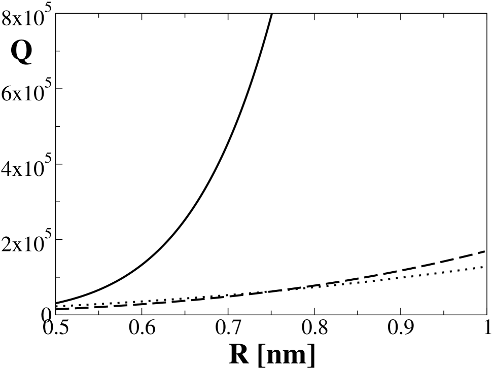
Figure 2: Quality factor for the three low-energy modes at $T=0$ and ${\cal L}=500$ nm as a function of tube radius $R$. The solid line depicts $Q_{F}$, the dashed line $Q_{L}$ and the dotted line $10^{-3}Q_{T}$.

However, as discussed in Sec. III.2, due to the smallness of $T^{*}$, the zero-temperature limit is actually not accessible experimentally, and one is always in the regime $T\gg T^{*}$. It is then interesting to evaluate the rate in the limit $X_{T}\gg 1$ but with $X_{T}^{1/3}X_{\cal L}\ll 1$, which corresponds to a regime in which the kinetic energy is much larger than the gap. For sufficiently short CNTs (or if one evaluates the rate at a larger wavevector than $\pi/{\cal L}$) the two inequalities can be satisfied simultaneously. In that case, we find from Eq. (83) that $\hbar\Gamma_{F}/k_{B}T^{*}\propto X_{\cal L}^{3}X_{T}^{2}$. The resulting $T^{2}$ power-law behavior for the temperature dependence of the flexural phonon decay rate is a prediction that should be observable with state-of-the art experiments.

V Electron-phonon coupling

In this section, we consider the effects of e-ph couplings in metallic single-wall CNTs. In contrast to the semiconducting case studied before, the coupling of phonons to electrons may contribute another decay channel beyond ph-ph interactions. Within lowest order perturbation theory, the two mechanisms are additive for the decay rates, and hence also for the inverse quality factors. Here, we only take into account the deformation potential as a source for e-ph coupling, as this coupling has a very significant strength.suzuura ; ademarti The phonons, described by the strain tensor $u_{ij}$, create the deformation potentialsuzuura

$$V_{e-ph}({\bf r})=V_{0}{\rm Tr}\left[u^{\rm lin}({\bf r})+u^{\rm nlin}({\bf r})\right],$$ (86)

where $V_{0}\approx 20$ eV (see Ref. suzuura, ). We will consider spinless electrons at a single Fermi point and eventually multiply by a factor 4 the final result for the rate, to take into account the electron spin and $KK^{\prime}$ degeneracies. Moreover, we only take into acccount electrons in the lowest transverse subband, with zero angular momentum. This is justified since the higher angular momentum states are separated by a large energy gap. Then, from the normal-mode representation in Appendix B, we observe that only the $L$ mode couples via the first term ($u^{\rm lin}$) in Eq. (86) (the coupling to the $F$ mode requires at least one electron in a higher angular momentum state), while the $F$ and $T$ phonons couple only via the second ($u^{\rm nlin}$) term, where two phonons are involved. The electronic contribution to the decay rate of the $T$ phonon is then expected to be weak, and we will focus on the decay of the $L$ and $F$ modes.

Let us start with the $L$ phonon with momentum $\hbar k$, where the relevant lowest-order self-energy diagram due to the first term in $V_{e-ph}$ corresponds to the electron-hole bubble. Its imaginary part, responsible for the phonon decay rate, is $\propto[\delta(\omega-v_{F}k)-\delta(\omega+v_{F}k)]$, where $\omega=v_{L}k$. (Note that we use a linearized dispersion for electrons.) Since the Fermi velocity is $v_{F}\approx 10^{6}$ m/sec $\gg v_{L}$, this condition can never be met, and only higher-order contributions can possibly lead to a phonon decay. This suggests that the decay rate of the $L$ phonon due to Eq. (86) is very small, and probably negligible against the ph-ph mechanism.

For the case of a $F$ phonon, the lowest-order contribution comes from the second term in Eq. (86), leading to a “fishbone” diagram with two electron lines and a phonon line. The corresponding imaginary-time self-energy is given by

$$\tilde{\Sigma}_{F}(\tau,k)=-\frac{1}{\hbar\rho_{M}}\left(\frac{3V_{0}}{2\pi R}\right)^{2}k^{2}\sum_{q}(k-q)^{2}{\cal G}(\tau,\omega_{0})\Pi_{e}(\tau,q),$$ (87)

with $\omega_{0}=\omega_{\rho}+\hbar(k-q)^{2}/2m$ and the 1D electron polarization functionmora

$$\Pi_{e}(\tau,q)=\frac{\omega_{e}}{2\pi v_{F}}\sum_{\xi=\pm}n(\xi\omega_{e})e^{\xi\omega_{e}\tau},$$

where $\omega_{e}=v_{F}|q|$. Following the same steps as in Sec. IV, we then find for the $T=0$ decay rate

$$\Gamma_{F}(k)\propto\sum_{q}\omega_{e}\delta(\omega_{F}(k)-\omega_{0}-\omega_{e}),$$

which yields the energy conservation condition

$$q^{2}-2qk+\sqrt{2}\frac{v_{F}|q|}{v_{L}R}=0.$$

For $q\neq 0$, this condition can only be met if $kR>v_{F}/(\sqrt{2}\ v_{L})$, i.e. only for short-wavelength phonons. Thus, for the long-wavelength phonons of interest here, the energy mismatch between electron-hole pair excitations and the phonon modes implies that again only higher-order terms can possibly generate a finite decay rate.

The above discussion therefore suggests that e-ph couplings via the deformation potential do not lead to significant decay rates of the gapless $L$ and $F$ modes. Their decay should then be dominated by the ph-ph interaction processes as described in Sec. IV.

VI Conclusions

In this paper, we have formulated and studied a general analytical theory of phonon-phonon interactions for low-energy long-wavelength acoustic phonons in carbon nanotubes. The continuum elasticity approach employed here reproduces the known dispersion relations of all gapless modes, including the flexural mode, $\omega_{F}(k)=\hbar k^{2}/2m$ with “effective mass” $m$. We have then included the most general cubic and quartic elastic nonlinearities allowed by symmetry. Remarkably, the relevant phonon-phonon scattering processes giving the dominant contributions to the decay rates are already found from the geometric nonlinearities (i.e. using the nonlinear strain tensor in a lowest-order expansion of the elastic energy density), and for a quantitative discussion of the decay rates, only the knowledge of the well-known Lamé coefficients (or equivalently of the sound velocities) is necessary.

We have provided a complete classification of all possible three-phonon processes involving gapless modes, along with the respective coupling constants. At the level of four-phonon processes we have focussed on the flexural modes, where a peculiarity is encountered, since the four-phonon processes lead to a singular behavior of the finite-temperature decay rate. The physical reason for this singularity is the proliferation of phonons at finite temperature, implying a divergent 1D density of flexural modes. Interactions effectively regularize this divergence and lead to a finite density. We have employed mean-field theory to quantitatively describe this mechanism, and found a dynamical temperature-dependent gap $\hbar\omega_{\rho}$ for flexural phonons. While this gap is in practice always below the thermal scale $k_{B}T$, it nevertheless leads to important consequences and allows to compute a well-defined decay rate for flexural phonons in low-order perturbation theory.

Using this approach, we have determined the decay rate and the quality factor for all long-wavelength gapless phonons in carbon nanotubes. We have also shown that electron-phonon interactions are ineffective in relaxing those modes due to a mismatch in energy scales. The reported quality factors ($Q$) are remarkably small, especially for thin CNTs, pointing to important phonon damping effects. Phonon-phonon interactions in CNTs are therefore significant and quite strong. Moreover, the values we have found are rather close to the typical $Q$ reported in recent experiments.bachtold Our predictions represent intrinsic upper bounds for $Q$. Such upper bounds can be valuable in assessing the predictions of approximate theories, or when interpreting experimental data in terms of phonon damping. We hope that our work will motivate further experimental and theoretical studies along this line.

Appendix A Curvature effects

In this appendix, we briefly discuss how to include curvature effects in the nonlinear elastic energy. To that end, we consider the metric tensor for the cylindrical surface, whose components ($i,j=x,y=1,2$),

$$g_{ij}=\sum_{n=x,y,z}t_{n,i}t_{n,j},$$

are expressed in terms of the ordinary scalar product of tangent vectors

$${\bf t}_{i}=\sum_{n}t_{n,i}({\bf r}){\bf e}_{n}(x)=\frac{\partial{\bf x}({\bf r})}{\partial x_{i}},$$

with ${\bf x}$ given in Eq. (2). The nonlinear strain tensor then follows equivalently from $2u_{ij}=g_{ij}-g_{ij}^{(0)}$, with the metric tensor $g_{ij}^{(0)}=\delta_{ij}$ of the undeformed cylinder. The local unit normal vector is ${\bf N}=({\bf t}_{x}\times{\bf t}_{y})/|{\bf t}_{x}\times{\bf t}_{y}|$, and the mean local curvature $\Omega$ of the cylinder is defined as

$$\Omega({\bf r})=\frac{1}{2}\sum_{ij}b_{ij}g^{ij},$$

where $g^{ij}$ is the inverse of $g_{ij}$, and the second fundamental form of the surface is

$$b_{ij}=\sum_{n=x,y,z}N_{n}\partial_{j}t_{n,i}.$$

To lowest order in the displacement fields $u_{n}$, the mean curvature is then given bysuzuura

$$\Omega=\Omega_{0}+\frac{u_{z}}{2R^{2}}+\frac{1}{2}\left(\frac{\partial^{2}u_{z}}{\partial x^{2}}+\frac{\partial^{2}u_{z}}{\partial y^{2}}\right),$$

where $\Omega_{0}=-1/2R$ is the curvature of the undeformed cylinder.

Curvature leads to an additional energy cost due to hybridization effects. One can model this in a phenomenological way by adding an additional term

$${\cal U}_{\rm curv}[u]=\kappa(\Omega-\Omega_{0})^{2}$$

to the elastic energy density, where $\kappa$ is a proportionality constant. Such effects turn out to be small unless one deals with ultrathin CNTs, but they provide gaps to flexural modes with angular momentum $|\ell|>1$. For $R\lesssim 1$ nm, these gaps are typically comparable in magnitudesuzuura to the breathing mode energy in Eq. (35).

Appendix B Normal mode representation of the strain tensor

In this appendix, we provide the explicit form of the strain tensor expressed in terms of the normal mode displacement field operators $u_{J}(k,\ell)$, see Eq. (24). We keep all $\ell=0$ modes ($L,T,B$), and the gapless flexural ($F$) modes with $\ell=\pm 1$. For the linear part of the strain tensor, see Eq. (5), we obtain from Eq. (23) the result

$$u^{\rm lin}({\bf r}) = \frac{1}{\sqrt{2\pi R}}\sum_{k}e^{iky}\Biggl{[}\left(\begin{array}[]{cc}-i\nu k&0\\ 0&ik\end{array}\right)u_{L}(k)+\left(\begin{array}[]{cc}0&ik/2\\ ik/2&0\end{array}\right)u_{T}(k)+\left(\begin{array}[]{cc}1/R&0\\ 0&\nu k^{2}R\end{array}\right)u_{B}(k)$$

$$+\frac{ik^{2}R}{\sqrt{2}}\sum_{\ell=\pm}e^{i\ell x/R}\left(\begin{array}[]{cc}\ell\nu&(1+\nu)kR\\ (1+\nu)kR&-\ell\end{array}\right)u_{F}(k,\ell)\Biggr{]},$$

while the nonlinear part (6) reads

$$u^{\rm nlin}({\bf r}) = \frac{1}{2\pi R}\sum_{k_{1},k_{2}}e^{i(k_{1}+k_{2})y}\Biggl{\{}\left(\begin{array}[]{cc}-\frac{\nu^{2}}{2}k_{1}k_{2}&0\\ 0&-\frac{1}{2}k_{1}k_{2}\end{array}\right)u_{L}(k_{1})u_{L}(k_{2})$$

$$+ \left(\begin{array}[]{cc}0&\frac{\nu}{2}k_{1}(k_{2}-k_{1})\\ \frac{\nu}{2}k_{1}(k_{2}-k_{1})&0\end{array}\right)u_{L}(k_{1})u_{T}(k_{2})$$

$$+ \left(\begin{array}[]{cc}\frac{1}{2R^{2}}&0\\ 0&-\frac{1}{2}k_{1}k_{2}\end{array}\right)\left[u_{T}(k_{1})u_{T}(k_{2})+u_{B}(k_{1})u_{B}(k_{2})\right]$$

$$+ \left(\begin{array}[]{cc}0&\frac{i}{2R}(k_{1}-k_{2})\\ \frac{i}{2R}(k_{1}-k_{2})&0\end{array}\right)u_{T}(k_{1})u_{B}(k_{2})+\left(\begin{array}[]{cc}-i\nu k_{1}/R&0\\ 0&i\nu k_{1}^{2}k_{2}R\end{array}\right)u_{L}(k_{1})u_{B}(k_{2})$$

$$+ \frac{1}{\sqrt{2}}\sum_{\ell_{2}=\pm}e^{ix\ell_{2}/R}\Biggl{[}\left(\begin{array}[]{cc}\nu^{2}\ell_{2}k_{1}k_{2}^{2}R&(1+\nu)k_{1}k_{2}/2\\ (1+\nu)k_{1}k_{2}/2&\ell_{2}(k_{2}+\nu k_{1})k_{1}k_{2}R\end{array}\right)u_{L}(k_{1})u_{F}(k_{2},\ell_{2})$$

$$+ \left(\begin{array}[]{cc}\nu k_{2}^{2}&-\ell_{2}k_{2}/2R\\ -\ell_{2}k_{2}/2R&-k_{1}k_{2}\end{array}\right)u_{T}(k_{1})u_{F}(k_{2},\ell_{2})+\left(\begin{array}[]{cc}i\nu\ell_{2}k_{2}^{2}&ik_{2}/2R\\ ik_{2}/2R&i\ell_{2}k_{1}k_{2}\end{array}\right)u_{B}(k_{1})u_{F}(k_{2},\ell_{2})\Biggr{]}$$

$$- \frac{k_{1}k_{2}}{4}\sum_{\ell_{1}\ell_{2}}e^{ix(\ell_{1}+\ell_{2})/R}\left(\begin{array}[]{cc}1&\frac{[\ell_{1}k_{1}+\ell_{2}k_{2}+\nu(\ell_{1}+\ell_{2})(k_{1}+k_{2})]R}{2}\\ \frac{[\ell_{1}k_{1}+\ell_{2}k_{2}+\nu(\ell_{1}+\ell_{2})(k_{1}+k_{2})]R}{2}&(1-\ell_{1}\ell_{2})\end{array}\right)$$

$$\times u_{F}(k_{1},\ell_{1})u_{F}(k_{2},\ell_{2})\Biggr{\}}.$$

For completeness, we also list the long-wavelength form of the three-phonon amplitudes involving the breathing mode:

$$A_{BBB} = \frac{K+\mu+2\xi_{1}+2\xi_{2}}{2R^{3}},$$

$$A_{BTT} = \frac{K+\mu}{2R^{3}},$$

$$A_{LBB} = \frac{ik_{1}}{R^{2}}[-K+\mu+3(1-\nu)\xi_{1}+(1-3\nu)\xi_{2}],$$

$$A_{LLB} = -\frac{k_{1}k_{2}}{R}[\nu K+3(1-\nu^{2})\xi_{1}+(2\nu-1-3\nu^{2})\xi_{2}],$$

$$A_{BFF} = -\delta_{\ell_{2},-\ell_{3}}\frac{(3K-\mu)k_{2}k_{3}}{4R}.$$

References

- (1) For recent reviews, see: T. Ando, J. Phys. Soc. Jpn. 74, 777 (2005); J.-C. Charlier, X. Blase, and S. Roche, Rev. Mod. Phys. 79, 677 (2007).
- (2) M.S. Dresselhaus and P.C. Eklund, Adv. Phys. 49, 705 (2000); M.S. Dresselhaus, G. Dresselhaus, R. Saito, and A. Jorio, Phys. Rep. 409, 47 (2005).
- (3) R. Rao, J. Menendez, C.D. Poweleit, and A.M. Rao, Phys. Rev. Lett. 99, 047403 (2007).
- (4) S. Roche, J. Jiang, L.E.F. Foa Torres, and R. Saito, J. Phys.: Condens. Matter 19, 183203 (2007).
- (5) P. Kim, L. Shi, A. Majumdar, and P.L. McEuen, Phys. Rev. Lett. 87, 215502 (2001); C. Yu, L. Shi, Z. Yao, D. Li, and A. Majumdar, Nano Lett. 5, 1842 (2005); M. Fujii, X. Zhang, H. Xie, H. Ago, K. Takahashi, T. Ikuta, H. Abe, and T. Shimizu, Phys. Rev. Lett. 95, 065502 (2005); H.-Y. Chiu, V.V. Deshpande, H.W.Ch. Postma, C.N. Lau, C. Miko, L. Forro, and M. Bockrath, Phys. Rev. Lett. 95, 226101 (2005).
- (6) S. Sapmaz, Ya.M. Blanter, L. Gurevich, and H.S.J. van der Zant, Phys. Rev. B 67, 235414 (2003).
- (7) B.J. LeRoy, S.G. Lemay, J. Kong, and C. Dekker, Nature 432, 371 (2004).
- (8) V. Sazonova, Y. Yaish, H. Üstünel, D. Roundy, T.A. Arias, and P.L. McEuen, Nature, 431, 284 (2004).
- (9) M. Huang, Y. Wu, B. Chandra, H. Yan, Y. Shan, T.F. Heinz, and J. Hone, Phys. Rev. Lett. 100, 136803 (2008).
- (10) A.K. Hüttel, B. Witkamp, M. Leijnse, M.R. Wegewijs, and H.S.J. van der Zant, preprint arXiv:0812.1769v1.
- (11) J. Hone, B. Batlogg, Z. Benes, A.T. Johnson, and J.E. Fischer, Science 289, 1730 (2000).
- (12) A. Gambetta, C. Manzoni, E. Menna, M. Meneghetti, G. Cerullo, G. Lanzani, S. Tretiak, A. Piryatinski, A. Saxena, R.L. Martin, and A.R. Bishop, Nature Physics 2, 515 (2006).
- (13) G.D. Sanders, C.J. Stanton, J.-H. Kim, K.-Y. Yee, Y.-S. Lim, E.H. Hároz, L.G. Booshehri, J. Kono, and R. Saito, preprint arXiv:0812.1953v1.
- (14) B. Babic, J. Furer, S. Sahoo, Sh. Farhangfar, and C. Schönenberger, Nano Lett. 3, 1577 (2003).
- (15) D. Garcia-Sanchez, A. San Paulo, M.J. Esplandiu, F. Perez-Murano, L. Forro, A. Aguasca, and A. Bachtold, Phys. Rev. Lett. 99, 085501 (2007).
- (16) S. Zippilli, G. Morigi, and A. Bachtold, Phys. Rev. Lett. 102, 096804 (2009).
- (17) T. Yamamoto, S. Watanabe, and K. Watanabe, Phys. Rev. Lett. 92, 075502 (2004).
- (18) N. Mingo and D.A. Broido, Phys. Rev. Lett. 95, 096105 (2005).
- (19) S. Zhang, M. Xia, S. Zhao, T. Xu, and E. Zhang, Phys. Rev. B 68, 075415 (2003).
- (20) B.I. Yakobson, C.J. Brabec, J. Bernholc, Phys. Rev. Lett. 76, 2511 (1996).
- (21) L. Wang, Q. Zheng, J.Z. Liu, and Q. Jiang, Phys. Rev. Lett. 95, 105501 (2005).
- (22) G.D. Mahan, Phys. Rev. B 65, 235402 (2002).
- (23) S.V. Goupalov, Phys. Rev. B 71, 085420 (2005).
- (24) L. Chico, R. Perez-Alvarez, and C. Cabrillo, Phys. Rev. B 73, 075425 (2006).
- (25) D. Walgraef, Eur. Phys. J. Special Topics 146, 443 (2007).
- (26) A.E.H. Love, A Treatise on the Mathematical Theory of Elasticity, 4th ed. (Dover, New York, 1944).
- (27) N. Yamaki, Elastic stability of circular cylindrical shells (North-Holland, Amsterdam, 1984).
- (28) R. Saito, T. Takeya, T. Kimura, G. Dresselhaus, and M.S. Dresselhaus, Phys. Rev. B 57, 4145 (1998).
- (29) G.D. Mahan and G.S. Jeon, Phys. Rev. B 70, 075405 (2004).
- (30) J.W. Jiang, H. Tang, B.S. Wang, and Z.B. Su, Phys. Rev. B 73, 235434 (2006).
- (31) D. Gunlycke, H.M. Lawler, and C.T. White, Phys. Rev. B 77, 014303 (2008).
- (32) J. Zimmermann, P. Pavone, and G. Cuniberti, Phys. Rev. B 78, 045410 (2008).
- (33) H. Suzuura and T. Ando, Phys. Rev. B 65, 235412 (2002).
- (34) A. De Martino and R. Egger, Phys. Rev. B 67, 235418 (2003).
- (35) L.D. Landau and E.M. Lifshitz, Elasticity Theory (Pergamon, Oxford, 1986).
- (36) C. Nisoli, P.E. Lammert, E. Mockensturm, and V.H. Crespi, Phys. Rev. Lett. 99, 045501 (2007).
- (37) O. Dubay, G. Kresse, and H. Kuzmany, Phys. Rev. Lett. 88, 235506 (2002); O. Dubay and G. Kresse, Phys. Rev. B 67, 035401 (2003).
- (38) R. Barnett, E. Demler, and E. Kaxiras, Phys. Rev. B 71, 035429 (2005); I. Milosevic, E. Dobardzic, and M. Damnjanovic, Phys. Rev. B 72, 085426 (2005).
- (39) N.W. Ashcroft and N.D. Mermin, Solid State Physics, Chapter 25 (Saunders, Philadelphia, 1975).
- (40) A.A. Maradudin and A.E. Fein, Phys. Rev. 128, 2589 (1962).
- (41) R.A. Cowley, Adv. Phys. 12, 421 (1963); Rep. Prog. Phys. 31, 123 (1968).
- (42) P. Keblinski and P.K. Schelling, Phys. Rev. Lett. 94, 209701 (2005); Y.-K. Kwon, S. Berber, and D. Tomanek, Phys. Rev. Lett. 94, 209702 (2005).
- (43) S.P. Hepplestone and G.P. Srivastava, Phys. Rev. B 74, 165420 (2006).
- (44) N. Mingo and D.A. Broido, Nano Lett. 5, 1221 (2005).
- (45) R. Orbach and L.A. Vredevoe, Physics 1, 92 (1964); R. Orbach, Phys. Rev. Lett. 16, 15 (1966).
- (46) P.G. Klemens, Phys. Rev. 148, 845 (1966).
- (47) H.J. Maris, Rev. Mod. Phys. 49, 341 (1977).
- (48) H.J. Maris and S.I. Tamura, Phys. Rev. B 47, 727 (1993).
- (49) M. Lax, P. Hu, and V. Narayanamurti, Phys. Rev. B 23, 3095 (1981).
- (50) S.I. Tamura, Phys. Rev. B 30, 610 (1984); ibid. 31, 2574 (1985).
- (51) N. Bonini, M. Lazzeri, N. Marzari, and F. Mauri, Phys. Rev. Lett. 99, 176802 (2007).
- (52) E. Mariani and F. von Oppen, Phys. Rev. Lett. 100, 076801 (2008).
- (53) J. Atalaya, A. Isacsson, and J.M. Kinaret, Nano Lett. 8, 4196 (2008).
- (54) D. Sánchez-Portal, E. Artacho, J.M. Soler, A. Rubio, and P. Ordejon, Phys. Rev. B 59, 12678 (1999).
- (55) J.P. Lu, Phys. Rev. Lett. 79, 1297 (1997).
- (56) J.C. Kimball, C.Y. Fong, and Y.R. Shen, Phys. Rev B 23, 4946 (1981).
- (57) B. Perrin, Phys. Rev. B 36, 4706 (1987).
- (58) F.H.L. Essler and I. Affleck, JSTAT P12006 (2004).
- (59) I.S. Gradsteyn and I.M. Ryzhik, Table of Integrals, Series, and Products (Academic Press, Inc., New York, 1980).
- (60) C. Mora, R. Egger, and A. Altland, Phys. Rev. B 75, 035310 (2007).