Comparison of three-dimensional and two-dimensional statistical
mechanics of shear layers for flow between two parallel plates.

Abstract

It is shown that the averaged velocity profiles predicted by statistical mechanics of point vortices and statistical mechanics of vortex lines are practically indistinguishable for a shear flow between two parallel walls.

I Introduction

It is known that statistical mechanics of point vortices describes surprisingly well the averaged velocity profiles of self-similar mixing layer. After development of statistical mechanics of vortex lines rf1 ; rf2 ; rf3 ; rf4 ; rf5 , where a vortex does not remain straight and is allowed to take wavy shapes in the course of motion, it appeared a concern that the above-mentioned feature of statistical mechanics of point vortices can be lost in three-dimensional theory. In this paper we show that this is not the case: the averaged velocity profiles predicted by statistical mechanics of point vortices and statistical mechanics of vortex lines are practically indistinguishable for a shear flow between two parallel walls.

II Averaged equations for flow between two plates

Consider a flow of ideal incompressible fluid between two parallel walls, $y$ is the coordinate normal to the walls, $-h\leq y\leq h$, $2h$ - the distance between the walls. The flow is modeled by motion of a large number of vortices (Fig.1). Flow is periodic in $x$-direction and $z$-direction. In the limit of infinite period in $z$-direction, the averaged velocity is parallel to the walls, does not depend on $x$ and has the only non-zero component, $u=u(y)$. Assuming that vortices have the same intensity and the total discharge is zero, one obtains for the stream function of the averaged flow, $\psi=\psi(y)$ ($u\equiv d\psi/dy$), the equation

$$\frac{d^{2}}{dy^{2}}\psi=-\sigma f(y),\quad\left.\frac{d}{dy}\psi\right|_{\pm h}=\pm U,$$ (1)

where $f(y)$ is the probability to find a vortex at the point $y$, $\sigma$ is the total vorticity per unit length in $x$-direction, $\sigma=-2U$. In the case of point vortices (Fig.1a), rf6 ; rf7

$$f\left(y\right)=\frac{e^{-\beta\sigma\psi\left(y\right)}}{\int_{-h}^{h}e^{-\beta\sigma\psi\left(y^{\prime}\right)}d^{2}y^{\prime}},$$ (2)

and equations Eq. (1), Eq. (2) form a closed system of equations. This system can be solved analytically. Parameter $\beta$ has the meaning of inverse temperature of vortex motion. It is determined by the initial energy of turbulent flow.
In the case of deforming vortex lines (Fig.1b), $f(y)$ is expressed through the solutions of the eigenvalue problem, rf4 ; rf5

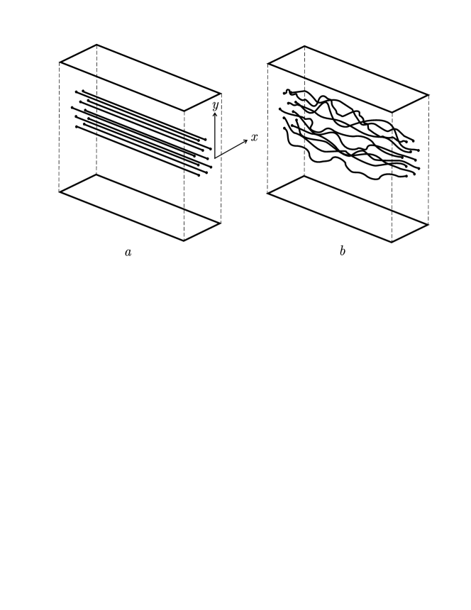
Figure 1: Two-dimensional flow of point vortices ($a$) and three-dimensional flow of vortex lines ($b$)

$$\Delta\varphi-\beta\sigma\psi\varphi=-\lambda\varphi,~{}~{}~{}\quad\left.\frac{d}{dy}\varphi\right|_{\pm h}=0,$$ (3)

$\lambda$ being the minimum eigenvalue. Similarly to quantum mechanics, $f(y)$ is proportional to the squared solution of the eigenvalue problem:

$$f(y)=\frac{\varphi^{2}(y)}{\int_{-h}^{h}\varphi^{2}(y)dy^{\prime}}.$$ (4)

We aim to compare solutions of Eq. (1),Eq. (2) and Eq. (1), Eq. (3), Eq. (4).

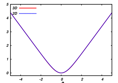
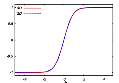
Figure 2: Stream function ($a$) and velocity ($b$) profiles for $\beta_{3D}=-1.0$ and $\beta_{2D}=-1.1374$

III Results and discussion

There is no reason to expect that the velocity profiles found from the two quite different system of equations, Eq. (1)-Eq. (2) and Eq. (1),Eq. (3), Eq. (4), coincide. Nevertheless, this turns out to be the case: the velocity profiles are practically indistinguishable. More precisely: for each $\beta$ from ”$3D$ problem” Eq. (1),Eq. (3), Eq. (4), there is $\beta$ from ”$2D$ problem” Eq. (1)-Eq. (2) for which the velocity profiles practically coincide.

System of equations Eq. (1)-Eq. (2) admits an analytical solution:

$$\psi=-\frac{1}{U\beta}\ln\cosh(Cy),$$ (5)

where the constant $C$ is determined from the boundary condition,

$$U+\frac{C}{U\beta}\tanh(Ch)=0.$$ (6)

For $h=\infty$, $C=-U^{2}\beta$ and Eq. (5) becomes:

$$\psi=-\frac{1}{U\beta}\ln\cosh(U^{2}\beta y).$$ (7)

All parameters of the flow can be normalized with respect to the wall velocity: $\psi\rightarrow\psi/U$, $\sigma\rightarrow\sigma/U$ and $\beta\rightarrow\beta U^{2}$. The dimension of the normalized $\beta$ is length^-1. The characteristic length, $\left|\beta\right|^{-1},$ is the width of the mixing layer.

Non-linear eigenvalue problem Eq. (1),Eq. (3), Eq. (4) was solved numerically using an iteration procedure. At each iteration step the system is being reduced to the Sturm-Liouville problem, that was solved with the Prüfer method (a shooting method based on oscillation rf8 ; rf9 ). For a given $\beta$ of vortex line flow, $\beta_{3D},$ one can choose $\beta$ of point vortex flow, $\beta_{2D},$ in such a way, that the velocity profiles are practically identical. This can be seen, for example, from Fig.2, where the velocity profiles and the stream function are shown for $\beta_{3D}=-1.0000$ and $\beta_{2D}=-1.1374$. The values of $\beta_{2D}$ and $\beta_{3D}$ for which the average velocity profiles coincide form a curve in the plane {$\beta_{2D},\beta_{3D}\}$ shown in Fig.3. This curve was found in the following way. For each $\beta_{3D}$ we seek $\beta_{2D}$ by the minimization of the sum

$$\sum_{i=1}^{N}w_{i}|u_{i}^{2D}-u_{i}^{3D}|,$$ (8)

where $u_{2D}$ and $u_{3D}$ are velocities in $2D$ and $3D$ problems, respectively, $N$ is the number of the mesh points. The weight coefficients, $w_{i},$ depend on the density of the mesh and the gradient of the velocity profile $u$. The distance between the walls, $h,$ was chosen large enough for the solution to be applicable.

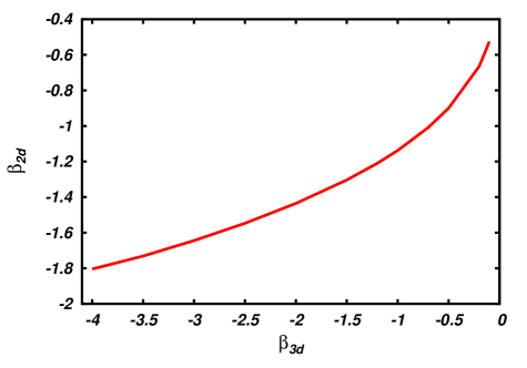
Figure 3: Two-dimensional inverse temperature $\beta_{2D}$ vs. three-dimensional inverse temperature $\beta_{3D}$

The parameters $\beta_{2D}$ and $\beta_{3D}$ have the meaning of the inverse temperature of two-dimensional and three-dimensional motions. The fact, that the same velocity profile corresponds to different $\beta_{2D}$ and $\beta_{3D}$, indicates that the corresponding temperatures of two-dimensional and three-dimensional motions are different. The temperature of two-dimensional motion has a simple physical meaning: this is an average area bounded by the vortex trajectory. The area has orientation. Accordingly, temperature may have both signs. Negative temperature of the flow considered corresponds to clockwise pass of the curls of the vortex trajectories rf1 . The physical meaning of temperature of three-dimensional vortex line motion is not known, therefore a physical interpretation of the graph $\beta_{2D}(\beta_{3D})$ is yet to be established. The result obtained seems an indication that for the shear flow between parallel walls three-dimensionality does not play an important role in formation of the averaged velocity profiles.

This paper has been published previously in the Russian journal rf9 that is not distributed in the West and on internet.

References

-
(1)
L. Akulenko and S. Nesterov.
High-precision methods in eigenvalue, problems and their applications.
Chapman & Hall/CRC, Boca Raton, 2005. - (2) V. Berdichevsky. Thermodynamics of Chaos and Order. Addison-Wesly-Longman, London, 1997.
- (3) V. Berdichevsky. Phys. Rev. E, 57:2885, 1998.
- (4) V. Berdichevsky. Int. J. Eng. Sci., 40:123, 2002.
- (5) V. Berdichevsky. Continuum Mech. Thermodyn., 19:133, 2007.
- (6) P.-L. Lions and A. Majda. Comm. Pure Appl. Math., 53:76, 2000.
- (7) D. Montgomery and G. Joyce. J. Plasma Phys, 10:107, 1973.
- (8) D. Montgomery and G. Joyce. Phys. Fluids, 17:1139, 1974.
- (9) J. Pryce. Numerical Solution of Sturm-Liouville Problems. Oxford University Press, New York, 1994.
-
(10)
L. Shirkov and V. Berdichevsky.
Izvestiya Vuzov. Severo-Kavkazkii Region,
Special Issue Actual problems of mathematical hydrodynamics, 2009.