Graph topologies induced by edge lengths

Abstract

Let $G$ be a graph each edge $e$ of which is given a length $\ell(e)$. This naturally induces a distance $d_{\ell}(x,y)$ between any two vertices $x,y$, and we let $|$G$|_{\ell}$ denote the completion of the corresponding metric space. It turns out that several well studied topologies on infinite graphs are special cases of $|$G$|_{\ell}$. Moreover, it seems that $|$G$|_{\ell}$ is the right setting for studying various problems. The aim of this paper is to introduce $|$G$|_{\ell}$, providing basic facts, motivating examples and open problems, and indicate possible applications.

Parts of this work suggest interactions between graph theory and other fields, including algebraic topology and geometric group theory.

1 Introduction

Let $G$ be a graph each edge $e$ of which is given a length $\ell(e)$. This naturally induces a distance $d_{\ell}(x,y)$ between any two vertices $x,y$, and we let $\ell\text{-}TOP(G)$, or $|$G$|_{\ell}$ for short, denote the completion of the corresponding metric space. It turns out that several well studied topologies on infinite graphs are special cases of $\ell\text{-}TOP$, see Section 1.1.

The space $|$G$|_{\ell}$ has already been considered, for special cases of $\ell$, by several authors who in most cases were apparently unaware of each other’s work: Floyd [20] used it in order to study Kleinian groups, and his work was taken up by Gromov who related it to hyperbolic graphs and groups, see Section 3.2. Benjamini and Schramm used it to prove that planar transient graphs admit harmonic Dirichlet functions [2], and to study sphere packings of graphs in $\mathbb{R}^{d}$ [3]. Carlson [9] studied the Dirichlet Problem at the boundary of $|$G$|_{\ell}$. Finally, the author used $|$G$|_{\ell}$ in [23] in order to prove the uniqueness of currents in certain electrical networks, see also Section 1.2.

The aim of this paper is to introduce $\ell\text{-}TOP$ in greater generality, providing definitions, motivating examples, basic facts and open problems, and indicate possible applications.

1.1 Interesting special cases of $\ell\text{-}TOP$

In Section 3 we will show how some well known topologies on graphs can be obtained as special cases of $\ell\text{-}TOP$ by choosing $\ell:E(G)\to\mathbb{R}_{>0}$ appropriately. The most basic such example is the Freudenthal compactification (also known as the end compactification) of a locally finite graph:

Theorem 1.1.

If $G$ is locally finite and $\sum_{e\in E(G)}\ell(e)<\infty$ then $|$G$|_{\ell}$ is homeomorphic to the Freudenthal compactification $|G|$ of $G$.

Another special case of $\ell\text{-}TOP$ is the Floyd completion of a locally finite graph, which in turn has as a special case the hyperbolic compactification of a hyperbolic graph in the sense of Gromov [28]. Other special cases include the topologies $ETOP$ and $MTOP$, which generalise the Freudenthal compactification to non-locally-finite graphs, for all graphs for which these topologies are metrizable; see Sections 2 and 3 for definitions and the details.

1.2 Infinite electrical networks

Infinite electrical networks are a useful tool in mathematics, for example in the study of random walks [34]. An electrical network $N$ has an underlying graph $G\$and a function $r:E(G)\to\mathbb{R}_{+}$ assigning resistances to the edges of $G$. If $G\$is finite, then the electrical current in $N$ —between two fixed vertices $p,q$ and with fixed flow value $I$— is the unique flow satisfying Kirchhoff’s second law. If $G\$is infinite then there may be several flows satisfying Kirchhoff’s second law, and one of the standard problems in the study of infinite electrical networks is to specify under what conditions such a flow is unique, see e.g. [39, 41].

In [23] we prove that if the sum of all resistances in a network $N$ is finite then there is a unique electrical current in $N$, provided we do not allow any flow to escape to infinity (see [23] for precise definitions):

Theorem 1.2 ([23]).

Let $N$ be an electrical network with $\sum_{e\in E(G)}r(e)<\infty$. Then there is a unique non-elusive $p$–$q$ flow with value $I$ and finite energy in $N$ that satisfies Kirchhoff’s second law.

The proof of Theorem 1.2 uses Theorem 1.1 and other basic facts about $\ell\text{-}TOP$ proved here (Section 4), as well as a result saying that, unless for some obvious obstructions, every flow satisfying Kirchhoff’s second law for finite cycles in an infinite network also satisfies Kirchhoff’s second law for infinite, topological circles in the space $|$G$|_{\ell}$ with $\ell:=r$.

1.3 The cycle space of an infinite graph and the homology of a continuum

The cycle space of a finite graph $G$ is the first simplicial homology group of $G$. This is a well studied object, and many useful results are known [13]. For infinite graphs many of these results fail even in the locally finite case, however, Diestel and Kühn [16, 17] proposed a new homology for an infinite graph $G$, called the topological cycle space $\mathcal{C}(G)$, that makes those results true also for locally finite graphs; an exposition of such results can be found in [11] or [13, Chapter 8.5]. The main innovation of the approach of Diestel and Kühn was to consider topological circles in the Freudenthal compactification $|G|$ of the graph, and use those circles as the building blocks of their cycle space $\mathcal{C}(G)$.

It is natural to wonder how this homology theory interacts with $|$G$|_{\ell}$: given an arbitrary function $\ell$ we can consider the topological circles in $|$G$|_{\ell}$ instead of those in $|G|$, and we may ask if the former circles can be the building blocks for a homology that retains the desired properties of $\mathcal{C}(G)$.

The attempts to answer the latter question led to a new homology, introduced in [22], that can be defined for an arbitrary metric space $X$ and has indeed important similarities to $\mathcal{C}(G)$, at least if $X$ is compact. This homology is described in Section 5, where we will also see an important example that motivates it.

1.4 Geodetic circles

As mentioned above, $|G|$ and the topological cycle space has led to generalisations of most well-known theorems about the cycle space of finite graphs to locally finite ones, however, there are cases where $|G|$ performs poorly: namely, problems in which a notion of length is inherent. We will see one such case here; another can be found in [23].

Let $G\$be a finite graph with edge lengths $\ell:E(G)\to\mathbb{R}_{>0}$. A cycle $C$ in $G$ is called $\ell$-geodetic if, for any two vertices $x,y\in C$, the length of at least one of the two $x$–$y$ arcs on $C$ equals the distance between $x$ and $y$ in $G$, where lengths and distances are considered taking edge lengths into account. It is easy to show (see [26]) that:

Theorem 1.3.

The cycle space of a finite graph $G\$is generated by its $\ell$-geodetic cycles.

It was shown in [26] that this theorem generalises to locally finite graphs using the topological cycle space, but only if the edge lengths respect the topology of $|G|$, where respecting the topology of $|G|$ means something slightly more general than $|$G$|_{\ell}$ being homeomorphic to $|G|$.

With $|$G$|_{\ell}$ we might be able to drop this restriction on $\ell$: we may ask whether for every $\ell:E(G)\to\mathbb{R}_{>0}$ the $\ell$-geodetic (topological) circles in $|$G$|_{\ell}$ —defined similarly to finite $\ell$-geodetic cycles— generate, in a sense, all other circles; more precisely, we conjecture that they generate the homology group alluded to in Section 1.3. See Section 6 for more.

1.5 Line graphs

The line graph $L(G)$ of a graph $G$ is defined to be the graph whose vertex set is the edge set of $G$ and in which two vertices are adjacent if they are incident as edges of $G$.

It is a well known fact that if a finite graph $G$ is eulerian then $L(G)$ is hamiltonian. This fact was generalised for locally finite graphs in [24, Section 10], where Euler tours and Hamilton cycles are defined topologically: a Hamilton circle is a homeomorphic image of $S^{1}$ in $|G|$ containing all vertices, and a topological Euler tour is a continuous mapping from $S^{1}$ to $|G|$ that traverses each edge precisely once.

We would like to generalise this fact to non-locally-finite graphs. In order to define topological Euler tours and Hamilton circles as above, we first have to specify some topology for those graphs. Interestingly, it turns out that we can obtain an elegant generalisation to non-locally-finite graphs, but only if different topologies are used for $G$ and $L(G)$:

Theorem 1.4.

If $G$ is a countable graph and $ETOP(G)$ has a topological Euler tour then $MTOP({L(G)})$ has a Hamilton circle.

(See Section 2.4 for the definition of $ETOP$ and Section 3.3 for the definition of $MTOP$.) This phenomenon can however be explained using $\ell\text{-}TOP$. If an assignment of edge lengths $\ell:E(G)\to\mathbb{R}_{>0}$ is given for a graph $G$, then it naturally induces an assignment of edge lengths $\ell_{L}$ to the edges of $L(G)$: let $\ell_{L}(f)=1/2(\ell(e)+\ell(d))$ for every edge $f$ of $L(G)$ joining the edges $e,d$ of $E(G)$ (to see the motivation behind the definition of $\ell_{L}$, think of the vertices of $L(G)$ as being the midpoints of the edges of $G$). In Section 3 we are going to show that if $\sum_{e\in E(G)}\ell(e)<\infty$, in which case $|$G$|_{\ell}$ is homeomorphic to $ETOP(G)$, then $|L(G)|_{\ell_{L}}$ is homeomorphic to $MTOP({L(G)})$, see Corollary 3.5. It could be interesting to try to generalise Theorem 1.4 for other assignments $\ell$.

We are going to prove Theorem 1.4 in Section 7.

2 Definitions and basic facts

Unless otherwise stated, we will be using the terminology of Diestel [13] for graph theoretical terms and the terminology of [1] and [30] for topological ones.

2.1 Metric spaces

In this subsection we recall some well-known facts for the convenience of the reader. A function $f$ from a metric space $(X,d_{x})$ to a metric space $(Y,d_{y})$ is uniformly continuous if for every $\epsilon>0$ there is a $\delta>0$, such that for every $x,y\in X$ with $d_{x}(x,y)<\delta$ we have $d_{y}(f(x),f(y))<\epsilon$. The following lemma follows easily from the definitions.

Lemma 2.1.

Let $f:M\to N$, where $M,N$ are metric spaces, be a uniformly continuous function. If $(x_{i})$ is a Cauchy sequence in $M$ then $(f(x_{i}))$ is a Cauchy sequence in $N$.

For every metric space $M$, it is possible to construct a complete metric space $M^{\prime}$, called the completion of $M$, which contains $M$ as a dense subspace. The completion $M^{\prime}$ of $M$ has the following universal property [36]:

If $$N f:M\to N f^{\prime}:M^{\prime}\to N f M^{\prime}$$ is a complete metric space and is a uniformly continuous function, then there exists a unique uniformly continuous function which extends . The space is determined up to isometry by this property (and the fact that it is complete). (1)

A continuum is a non-empty, compact, connected metric space.

2.2 Topological paths, circles, etc.

A circle in a topological space $X$ is a homeomorphic copy of the unit circle $S^{1}$ of $\mathbb{R}^{2}$ in $X$. An arc $R$ in $X$ is a homeomorphic image of the real interval $[0,1]$ in $X$. Its endpoints are the images of $0$ and $1$ under any homeomorphism from $[0,1]$ to $R$. If $x,y\in R$ then $xRy$ denotes the subarc of $R$ with endpoints $x,y$. A topological path in $X$ is a continuous map from a closed real interval to $X$.

A circlex is a singular 1-simplex traversing a circle $C$ once and in a straight manner; in other words, a continuous mapping $\sigma:[0,1]\to C$ that is injective on $(0,1)$ and satisfies $\sigma(0)=\sigma(1)$.

Let $\sigma:[a,b]\to X$ be a topological path in a metric space $(X,d)$. For a finite sequence $S=s_{1},s_{2},\ldots,s_{k}$ of points in $[a,b]$, let $\ell(S):=\sum_{1\leq i<k}d(\sigma(s_{i}),\sigma(s_{i+1}))$, and define the length of $\sigma$ to be $\ell(\sigma):=\sup_{S}\ell(S)$, where the supremum is taken over all finite sequences $S=s_{1},s_{2},\ldots,s_{k}$ with $a=s_{1}<s_{2}<\ldots<s_{k}=b$. If $C$ is an arc or a circle in $(X,d)$, then we define its length $\ell(C)$ to be the length of a surjective topological path $\sigma:[0,1]\to C$ that is injective on $(0,1)$; it is easy to see that $\ell(C)$ does not depend on the choice of $\sigma$.

We are going to need the following well-known facts.

Lemma 2.2 ([29, p. 208]).

The image of a topological path with endpoints $x,y$ in a Hausdorff space $X$ contains an arc in $X$ between $x$ and $y$.

Lemma 2.3 ([1]).

A continuous bijection from a compact space to a Hausdorff space is a homeomorphism.

2.3 $\ell\text{-}TOP$

Every graph $G\$in this paper is considered to be a 1-compex, which means that the edges of $G$ are homeomorphic copies of the real unit interval. A half-edge of a graph $G$ is a connected subset of an edge of $G$.

Fix a graph $G$ and a function $\ell:E(G)\to\mathbb{R}_{>0}$, and for each edge $e\in E(G)$ fix an isomorphism $\sigma_{e}$ from $e$ to the real interval $[0,\ell(e)]$; by means of $\sigma_{e}$ any half-edge $f$ with endpoints $a,b$ obtains a length $\ell(f)$, namely $\ell(f):=|\sigma_{e}(a)-\sigma_{e}(b)|$.

We can use $\ell$ to define a distance function on $G$: for any $x,y\in V(G)$ let $d_{\ell}(x,y)=\inf\{\ell(P)\mid P\text{ is an $x$\text{--}$y$~{}path}\}$, where $\ell(P):=\sum_{e\in E(P)}\ell(e)$. For points $x,y\in G$ that might lie in the interior of an edge we define $d_{\ell}(x,y)$ similarly, but instead of graph-theoretical paths we consider arcs in the 1-complex $G$: let $d_{\ell}(x,y)=\inf\{\ell(P)\mid P\text{ is an $x$\text{--}$y$~{}arc}\}$, where $\ell(P)$ is now the sum of the lengths of the edges and maximal half-edges in $P$; note that this sum equals the length of $P$ as defined in Section 2.2 (for metric spaces in general). By identifying any two vertices $x,x^{\prime}$ of $G$ for which $d_{\ell}(x,x^{\prime})=0$ holds we obtain a metric space $(\overline{G},d_{\ell})$. Note that if $G\$is locally finite then $\overline{G}=G$. Let $|$G$|_{\ell}$ be the completion of $(\overline{G},d_{\ell})$.

The boundary points of $G$ are the elements of the set $\partial^{\ell}G:=|$G$|_{\ell}\backslash\pi(\overline{G})$, where $\pi$ is the canonical embedding of $\overline{G}$ in its completion $|$G$|_{\ell}$.

For a subspace $X$ of $|$G$|_{\ell}$ we write $E(X)$ for the set of edges contained in $X$, and we write $\mathaccent 28695{E}(X)$ for the set of maximal half-edges contained in $X$; note that $\mathaccent 28695{E}(X)\supseteq E(X)$. Similarly, for a topological path $\tau$ we write $E(\tau)$ for the set of edges contained in the image of $\tau$.

In this paper we will often encounter special cases of $|$G$|_{\ell}$ that induce some other well known topology on some space $G^{\prime}$ containing $G$, e.g. the Freudenthal compactification of $G$. In order to be able to formally state the fact that the two topologies are the same, we introduce the following notation. Let $X,X^{\prime}$ be topological spaces that contain another topological space $G$. We will write $X\approx_{G}X^{\prime}$, or simply $X\approx X^{\prime}$ if $G$ is fixed, if the identity on $G$ extends to a homeomorphism between $G^{\prime}$ and $G^{\prime\prime}$.

If $G\$is locally finite then we could also define $|$G$|_{\ell}$ by the following definition, which is equivalent to the above as the interested reader will be able to check (using, perhaps, Lemma 4.1 below). Let $R,L$ be two rays —see Section 2.4 below for the definition of a ray— of finite total length in $G$; we say that $R$ and $L$ are equivalent, if there is a third ray of finite total length that meets both $R$ and $L$ infinitely often. Now define $\partial G$ to be the set of equivalence classes of rays of finite total length in $G$ with respect to this equivalence relation, and let $|$G$|_{\ell}:=G\cup\partial G$; to extend the metric $d_{\ell}$ from $G$ to all of $|$G$|_{\ell}$, let the distance $d_{\ell}(x,y)$ between two points $x,y$ in $\partial G$ be the infimum of the lengths of all double rays with one ray in $x$ and one ray in $y$, and let $d_{\ell}(x,v)$ for $x\in\partial G$ and $v\in G$ be the infimum of the lengths of all rays in $x$ starting at the point $v$.

2.4 Ends, the Freudenthal compactification and the topological cycle space

Let $G\$be a graph fixed thgoughout this section.

A $1$-way infinite path is called a ray, a $2$-way infinite path is a double ray. A tail of the ray $R$ is a final subpath of $R$. Two rays $R,L$ in $G$ are vertex-equivalent if no finite set of vertices separates them; we denote this fact by $R\approx_{G}L$, or simply by $R\approx L$ if $G$ is fixed. The corresponding equivalence classes of rays are the vertex-ends of $G$. We denote the set of vertex-ends of $G$ by $\Omega=\Omega(G)$. A ray belonging to the vertex-end $\omega$ is an $\omega$-ray. Similarly, two rays are edge-equivalent if no finite set of edges separates them and we call the corresponding equivalence classes the edge-ends of $G$ and let $\Omega^{\prime}(G)$ denote the set of edge-ends of $G$. In a locally finite graph $G\$any two rays are edge-equivalent if and only if they are vertex-equivalent, and we will simply call the corresponding equivalence classes the ends of $G\$.

We now endow the space consisting of $G$, considered as a 1-complex, and its edge-ends with the topology $ETOP(G)$. Firstly, every edge $e\in E(G)$ inherits the open sets corresponding to open sets of $[0,1]$. Moreover, for every finite edge-set $S\subset E(G)$, we declare all sets of the form

$$C\cup\Omega^{\prime}(C)\cup E^{\prime}(C)$$ (2)

to be open, where $C$ is any component of $G-S$ and $\Omega^{\prime}(C)$ denotes the set of all edge-ends of $G$ having a ray in $C$ and $E^{\prime}(C)$ is any union of half-edges $(z,y]$, one for every edge $e=xy$ in $S$ with $y$ lying in $C$. Let $ETOP^{\prime}(G)$ denote the topological space of $G\cup\Omega^{\prime}$ endowed with the topology generated by the above open sets. Moreover, let $ETOP(G)$ denote the space obtained from $ETOP^{\prime}(G)$ by identifying any two points that have the same open neighbourhoods. If a point $x$ of $ETOP(G)$ resulted from the identification of a vertex with some other points (possibly also vertices), then we will, with a slight abuse, still call $x$ a vertex. It is easy to see that two vertices $v,w$ of $G\$are identified in $ETOP(G)$ if and only if there are infinitely many edge-disjoint $v$–$w$ paths.

If $G\$is locally finite then $ETOP^{\prime}(G)$ and $ETOP(G)$ coincide, and it can be proved (see [15]) that $ETOP(G)$ is the Freudenthal compactification [21] of the 1-complex $G$ in that case. It is common in recent literature to denote this space by $|G|$ if $G\$is locally finite, and we will comply with that convention.

The study of $|G|$, in particular of topological circles therein, has been a very active field recently. It has been demonstrated by the work of several authors ([4, 5, 6, 7, 8, 16, 17, 25, 24, 26, 40]) that many well known results about paths and cycles in finite graphs can be generalised to locally finite ones if the classical concepts of path and cycle are interpreted topologically, i.e. replaced by the concepts of a (topological) arc and circle in $|G|$; see [13, Section 8.5] or [11] for an exposition. An example of such a topological circle is formed by a double ray both rays of which converge to the same end, together with that end. There can however be much more exciting circles in $|G|$: in Figure 1, the infinitely many thick double rays together with the continuum many ends of the graph combine to form a single topological circle $W$, the so-called wild circle, discovered by Diestel and Kühn [16]. The double rays are arranged within $W$ like the rational numbers within the reals: between any two there is a third one; see [16] for a more precise description of $W$.

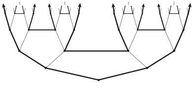
Figure 1: The ‘wild’ circle, formed by infinitely many (thick) double rays and continuum many ends. In this drawing it bounds the outer face of the graph.

We finish this section with a basic fact about infinite graphs that we will use later. A comb in $G\$is the union of a ray $R$ (called the spine of the comb) with infinitely many disjoint finite paths having precisely their first vertex on $R$. A subdivided star is the union of a (possibly infinite) set of finite paths that have precisely one vertex in common.

Lemma 2.4 ([13, Lemma 8.2.2]).

Let $U$ be an infinite set of vertices in a connected graph $G$. Then $G$ contains either a ray $R$ and infinitely many pairwise disjoint $U$–$R$ paths or a subdivided star with infinitely many leaves in $U$.

3 Special cases of $\ell\text{-}TOP$

3.1 The Freudenthal compactification and $ETOP(G)$

We start this section by proving Theorem 1.1, which states that the Freudenthal compactification of a locally finite graph is a special case of $|$G$|_{\ell}$. Since for a locally finite graph $G\$the Freudenthal compactification coincides with the topology $ETOP(G)$, Theorem 1.1 is a corollary of the following.

Theorem 3.1.

If $G$ is countable and $\sum_{e\in E(G)}l(e)<\infty$ then $|$G$|_{\ell}\approx ETOP(G)$.

Proof.

The proof consists of two steps: in the first step we put a metric $d$ on $ETOP(G)$ similar to $d_{\ell}$ and show that this metric induces $ETOP(G)$, while in the second step we show that the corresponding metric space is the completion of $(\overline{G},d_{\ell})$ using property (1) (the space $\overline{G}$ was introduced in Section 2.3, and property (1) in Section 2.1). As the interested reader can check, it is also possible, and not harder, to prove Theorem 3.1 by more direct arguments, without using (1).

For the first step, define $d(x,y):=d_{\ell}(x,y)$ for every $x,y$ in the 1-complex $G$. If $x\in\Omega^{\prime}(G)$ and $y\in V(G)$ (respectively $y\in\Omega^{\prime}(G)$), then let $d(x,y)$ be the infimum of the lengths of all rays in $x$ starting at $y$ (resp. all $x$–$y$ double rays), where the length of a (double-)ray $R$ is taken to be $\sum_{e\in E(R)}\ell(e)$. Define $d(x,y)$ similarly for the case that $x\in\Omega^{\prime}(G)$ and $y$ lies in an edge. It is easy to check that $d$ is indeed a metric. We claim that $d$ induces the topology $ETOP(G)$. To prove this we need to show that for any open set $O$ of $ETOP(G)$ and any $x\in O$ there is a ball $B\ni x$ with respect to $d$ contained in $O$ and vice versa.

So suppose firstly that $O$ is a basic open set in $ETOP(G)$ with respect to the finite edge-set $F$, and pick an $x\in O$. If $x$ is an inner point of some edge $f\in F$, then it is easy to find a ball of $x$ contained in $f\cap O$, so we may assume that $x$ is not such a point. Let $r=\min_{e\in F}\ell(e)$. Then, the ball $B_{d}(x,r)$ is contained in $O\cup\bigcup F$, since for any point $y$ in $G$ that $F$ separates from $x$ we have $d(x,y)\geq r$ by the definition of $d$. Thus, easily, there is an $r^{\prime}\leq r$, depending on $O\cap\bigcup F$, such that $B_{d}(x,r^{\prime})\subseteq O$.

Next, pick a ball $U=B_{d}(x,r)$ and a $y\in U$. We want to find an open set $O$ in $ETOP(G)$ such that $y\in O\subseteq U$. Easily, we can again assume that $y$ is not an inner point of an edge. Moreover, we may assume without loss of generality that $x=y$. As $\sum_{e\in E(G)}l(e)<\infty$ holds, there is a finite edge set $F$ such that the sum $\sum_{e\in E(G)\backslash F}\ell(e)$ of the lengths of all edges not in $F$ is less than $r$. We claim that any basic open set $O$ of $ETOP(G)$ with respect to the edge-set $F$ that contains $x$ is a subset of $U$. Indeed, for any point $w\in O$ we have $d(x,w)<r$ because the sum of the lengths of all edges in $O$, and thus also in any path or ray in $O$, is less than $r$.

Thus $d$ induces $ETOP(G)$ as claimed. It is easy to check that $d$ is a pseudometric on the set of points $M$ in $ETOP(G)$. To see that it is a metric, note that for any two points $w,z$ in $M$ that can be separated by a finite edge set $F$ we have $d(w,z)\geq\min_{e\in F}\ell(e)>0$. The second step of our proof is to show that the metric space $(M,d)$ is isometric to the completion of $(\overline{G},d_{\ell})$, that is, $|$G$|_{\ell}$, and we will do so using (1).

We first need to show that $(M,d)$ is complete. To do so, let $(x^{\prime}_{i})$ be a Cauchy sequence in $(M,d)$. If there is an edge containing infinitely many of the $x^{\prime}_{i}$ then it is easy to see that $(x^{\prime}_{i})$ has a limit, so assume this is not the case. Then, as $\sum_{e\in E(G)}\ell(e)<\infty$, it is possible to replace every $x^{\prime}_{i}$ that is an inner point of an edge by a vertex $x_{i}$ close enough to $x^{\prime}_{i}$, to obtain a sequence of vertices $(x_{i})$ equivalent to $(x^{\prime}_{i})$. If the set $\{x_{i}\mid{i\in\mathbb{N}}\}$ is finite then one of its elements is a limit of $(x^{\prime}_{i})$. If it is infinite, then by Lemma 2.4 there is either a comb with all teeth in $(x_{i})$ or a subdivision of an infinite star with all leaves in $(v_{i})$. If the former is the case, then $(x_{i})$, and thus $(x^{\prime}_{i})$, converges to the limit of the comb, and if the latter is the case then both sequences converge to the center of the star. This proves that $(M,d)$ is complete.

It is easy to see that two vertices $v,w$ of $G\$are identified in $ETOP(G)$ if and only if there are infinitely many edge-disjoint $v$–$w$ paths, which is the case if and only if $v$ and $w$ are identified in $\overline{G}$. Thus we can define a canonical projection $\pi:\overline{G}\to ETOP(G)$, mapping an inner point of an edge to itself, and mapping an equivalence class in $\overline{G}$ of vertices of $G$ to the element of $M$ containing all these vertices. It is straightforward to check that $\pi$ is an isometry and that its image is dense in $ETOP(G)$.

In order to use (1), let $(X,d_{x})$ be a complete metric space, and let $f:\overline{G}\to X$ be a uniformly continuous function. In order to extend $f\circ\pi^{-1}:M\to X$ into a uniformly continuous function $f^{\prime}:M\to X$, given $\omega\in\Omega^{\prime}(G)\cap ETOP(G)$ pick an $\omega$-ray $R$, and let $v_{1},v_{2},\ldots$ be the sequence of vertices in $R$. As $\sum_{e\in R}\ell(e)<0$ it is easy to check that $(v_{i})$ is a Cauchy sequence, and thus by Lemma 2.1 $(f(v_{i}))$ is a Cauchy sequence in $X$. Let $x$ by the limit of $(f(v_{i}))$ in $X$ and put $f^{\prime}(\omega)=x$. It is now straightforward to check that $f^{\prime}$ is uniformly continuous. Moreover, as for any $\omega\in\Omega^{\prime}(G)\cap ETOP(G)$ there are vertices $x_{i}$ (e.g. the vertices of an $\omega$-ray) such that $d(\omega,x_{i})$ becomes arbitrarily small, it is easy to check that this $f^{\prime}$ is the only (uniformly) continuous extension of $f\circ\pi^{-1}$. Thus, by (1), $(M,d)$ is isometric to the completion of $(\overline{G},d_{\ell})$, that is, $|$G$|_{\ell}$. ∎

Theorem 3.1 plays an important role in the proof of Theorem 1.2. A further application is an easy proof of the following known fact (see [13, Proposition 8.5.1] for the locally finite case or [37, Section 2.1] for the general case).

Corollary 3.2.

If $G\$is a connected countable graph then $ETOP(G)$ is compact.

Proof.

It is not hard to see that if an assignment $\ell:E(G)\to\mathbb{R}_{>0}$ satisfies $\sum_{e\in E(G)}\ell(e)<\infty$ then $|$G$|_{\ell}$ is totally bounded. The assertion now follows from Theorem 3.1 and the fact that every complete totally bounded metric space is compact. ∎

It is natural to wonder whether the condition $\sum_{e\in E(G)}\ell(e)<\infty$ in Theorem 3.1 can be replaced by some weaker but still elegant condition. However, this does not seem to be possible, as indicated by the following example: Figure 2 shows an 1-ended locally finite graph $G\$and an assignment of lengths such that for every $\epsilon$ there are only finitely many edges longer than $\epsilon$. Still, as the interested reader can check, $|$G$|_{\ell}$ does not induce $|G|$ in this case. Even worse, as we move along the bottom horizontal ray of this graph, the distance to the limit of the upper horizontal ray grows larger, although the two rays converge to the same point in $|G|$.

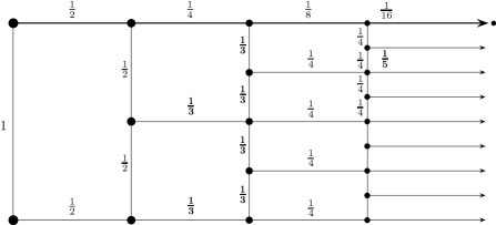
Figure 2: A somewhat surprising example.

3.2 The hyperbolic compactification

In a seminal paper [28] Gromov introduced the notions of a hyperbolic graph and a hyperbolic group, and defined for each such graph a compactification $\mathcal{H}(G)$, called the hyperbolic compactification of $G$, that refines $|G|$. It turns out that this space $\mathcal{H}(G)$ is also a special case of $|$G$|_{\ell}$.

For the definitions of hyperbolic graphs and their compactification the interested reader is referred to [38]. An example of a hyperbolic graph $G\$is shown in Figure 3. Other examples include all tessellations of the hyperbolic plane. The study of finitely generated groups whose Cayley graphs are hyperbolic is a very active research field with many applications, see [31] for a survey.

Another notion related to the hyperbolic compactification is that of the Floyd completion. To define it, let $G\$be a locally finite graph and let $f:\mathbb{N}\to\mathbb{R}_{>0}$ be a summable function, i.e. $\sum_{n\in\mathbb{N}}f(n)<\infty$, that does not decrease faster than exponentially; formally, there is a constant $\lambda>0$ such that $\lambda f(n-1)\leq f(n)\leq f(n-1)$ for every $n>0$. Now fix a vertex $p$ of $G\$and assign to each edge $e\in E(G)$ the length $\ell(e):=f(d(p,e))$, where $d(p,e)$ denotes the graph-theoretical distance, i.e. the least number of edges that form a path from $p$ to one of the endvertices of $e$. We define the Floyd completion $\mathcal{H}_{f}(G)$ of $G\$(with respect to $f$) to be $|$G$|_{\ell}$ for this $\ell$. Floyd introduced this space in [20] and used it in order to study Kleinian groups. Gromov showed ([28, Corollary 7.2.M]) that if $G\$is hyperbolic then $f$ can be chosen in such a way (in addition to the above properties) that the Floyd completion coincides with the hyperbolic compactification (see [10] for a more detailed exposition):

Theorem 3.3 ([28]).

For every locally finite hyperbolic graph $G\$there is a constant $\epsilon\in\mathbb{R}_{+}$ such that the hyperbolic compactification $\mathcal{H}(G)$ of $G\$is homeomorphic to its Floyd completion $\mathcal{H}_{f}(G)$ for $f(n):=\exp({-\epsilon n})$.

Since the Floyd completion is explicitly defined as a special case of $|$G$|_{\ell}$, we immeadiately obtain

Corollary 3.4.

For every locally finite hyperbolic graph $G\$there is $\ell:E(G)\to\mathbb{R}_{>0}$ such that the hyperbolic compactification $\mathcal{H}(G)$ of $G\$is homeomorphic to $|$G$|_{\ell}$.

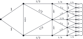
Figure 3: A hyperbolic graph $G$. Each level $i$ of $G$ is a perpendicular path $P_{i}$ of $2^{i}$ edges from the upper to the bottom horizontal ray. The hyperbolic boundary of this graph, i.e. $\mathcal{H}(G)\backslash G$, is homeomorphic to a closed real interval, and any two disjoint horizontal rays converge to distinct points in this boundary.

In the graph of Figure 3 for example, if we let $f(n):=2^{-n}$ then $\mathcal{H}_{f}(G)$ will be homeomorphic to $\mathcal{H}(G)$. (Note however that not any exponentially decreasing $f$ would do; if we let $f(n):=4^{-n}$ for instance, then $\mathcal{H}_{f}(G)$ will be homeomorphic to $|G|$.)

Intuitively, hyperbolic graphs are characterised by the property that for any two geodetic rays $R,L$ starting at a vertex $x$ of the graph graph, one of two possibilities must occur: either there is a constant $C$ such that each vertex of $R$ is at most $C$ edges apart from some vertex of $L$, or $R$ and $L$ diverge exponentially; that is, the minimum length of an $R$–$L$ path $P_{r}$ outside the ball of radius $r$ around $x$ grows exponentially with $r$. (See [38, Definition 1.7] for a more precise statement of this fact.) The function $f$ in Theorem 3.3 is chosen in such a way, that for any two rays $R,L$ as above that diverge exponentially the paths $P_{r}$ are assigned lengths that are bounded away from 0, and thus $R$ and $L$ will converge to distinct points in $\mathcal{H}_{f}(G)$.

3.3 Non-locally-finite graphs

The topology $ETOP(G)$ we used in Section 3.1 compactifies $G\$by its edge-ends. A further popular [14] possibility to extend $|G|$ to a non-locally-finite graph $G\$is the topology $MTOP({G})$, which consists of $G\$and its vertex-ends. As we shall see, $MTOP({G})$ is also a special case of $|$G$|_{\ell}$. To define $MTOP({G})$ we consider each edge of $G\$to be a copy of the real interval $[0,1]$, bearing the corresponding metric and topology. The basic open neighbourhoods of a vertex $v$ are, then, taken to be the open stars of radius $\epsilon$ centered at $v$ for any $\epsilon<1$. For a vertex-end $\omega\in\Omega(G)$ we declare all sets of the form

$$\widehat{C_{\epsilon}}(S,\omega):=C(S,\omega)\cup\Omega(S,\omega)\cup\mathaccent 28695{E}_{\epsilon}(S,\omega)$$

to be open, where $S$ is an arbitrary finite subset of $V(G)$, $C(S,\omega)$ is the unique component of $G-S$ containing a ray in $\omega$, and $\mathaccent 28695{E}_{\epsilon}(S,\omega)$ is the set of all inner points of $S-C(S,\omega)$ edges at distance less than $\epsilon$ from their endpoint in $C(S,\omega)$.

As stated in Section 1.5, if $G$ is a countable graph and $\sum_{e\in E(G)}\ell(e)<\infty$ for some $\ell:E(G)\to\mathbb{R}_{>0}$, then $|L(G)|_{\ell_{L}}\approx MTOP({L(G)})$; this is implied by the following statement, which can be proved by imitating the proof of Theorem 3.1.

Corollary 3.5.

Let $G$ be a countable graph, $v_{1},v_{2},\ldots$ an enumeration of the vertices of $G$, and for every edge $v_{i}v_{j}$ let $\ell^{\prime}(v_{i}v_{j})=1/2(\ell_{i}+\ell_{j})$ where $(\ell_{i})_{i\in\mathbb{N}}$ is a sequence of positive real numbers with $\sum_{i}\ell_{i}<\infty$. Then $|G|_{\ell^{\prime}}\approx MTOP({G})$.

This shows that $MTOP({G})$ is a special case of $|$G$|_{\ell}$ if $G$ is countable, but in fact we can do better and drop the latter requirement as long as $MTOP({G})$ is metrizable. The graphs $G$ for which this is the case were characterised by Diestel:

Theorem 3.6 ([14]).

If $G$ is connected then $MTOP($G$)$ is metrizable if and only if $G$ has a normal spanning tree.

We can show that $MTOP({G})$ is a special case of $|$G$|_{\ell}$ for all those graphs:

Theorem 3.7 ([14, Theorem 3.1]).

Let $G$ be a connected graph. Then, there is $\ell:E(G)\to\mathbb{R}_{>0}$ such that $|$G$|_{\ell}\approx MTOP($G$)$ if and only if $MTOP($G$)$ is metrizable.

Proof (sketch)..

The forward implication is trivial. For the backward implication we will proceed similarly to the proof of Theorem 3.1. So suppose that $MTOP($G$)$ is metrizable. Then, by Theorem 3.6, $G$ has a normal spanning tree $T$. For a vertex $v\in V(G)$ let $r(e)$ be the level of $v$ in $T$, that is, the number of edges in the path in $T$ from the root of $T$ to $v$. We now specify the required edge lengths $\ell$: for every edge $e=uv$, where $r(u)<r(v)$, let $\ell(e)=\sum_{r(u)<n\leq r(v)}1/2^{n}$. Now define a metric $d$ on the point set of $MTOP$($G$) as follows. For every $x,y\in V(G)\cup\Omega(G)$, let $d(x,y)=\sum_{e\in P}\ell(e)$, where $P$ is the $x$–$y$ path in $T$ if both $x,y$ are vertices, and $P$ is the $x$-$y$ (double-)ray in $T$ if one or both of $x,y$ is a vertex-end. Define $d(x,y)$ for inner points of edges similarly. Clearly, $d(x,y)=d_{\ell}(x,y)$ if $x,y\in G$. It is straightforward to check that $d$ induces $MTOP($G$)$; see [14, Theorem 3.1] for more details. Now similarly to the proof of Theorem 3.1 one can show that $MTOP($G$)$ is the completion of $(\overline{G},d_{\ell})$ using (1). ∎

A further topology for infinite (non-locally-finite) graphs that might be obtainable as a special case of $\ell\text{-}TOP$ is the topology of metric ends. These are defined similarly to vertex-ends, only the role of finite vertex separators is now played by separators of finite diameter with respect to the usual edge-counting metric; see [32, 33] for more details. We can thus ask:

Problem 3.1.

Does every graph $G\$admit an assignment $\ell:E(G)\to\mathbb{R}_{>0}$ such that the identity on $G\$induces a bijection between $\partial^{\ell}G$ and the set of metric ends of $G$? If yes, are the corresponding topologies homeomorphic?

The end compactification $|G|$ of a locally finite graph $G\$has allowed the generalisation of many important facts about finite graphs to infinite, locally finite ones, see [12]. When trying to extend those results further to non-locally-finite graphs however, one often has to face the dilemma of which topology to use, as there are several ways to generalise $|G|$ to a non-locally-finite graph. In this section we considered two of these ways, namely the spaces $ETOP(G)$ and $MTOP$($G$), and “unified” them by showing that they are both special cases of $\ell\text{-}TOP$ (Theorem 3.1 and Theorem 3.7). This unification suggests a solution to the aforementioned dilemma: instead of fixing a topology on the non-locally-finite graph, one could try to prove the desired result for all instances of $\ell\text{-}TOP$, or at least for a large subclass of them like e.g. the compact ones, which would then lead to corollaries for the specific spaces. This approach will be exemplified in Section 5.1.

4 Basic facts about $|$G$|_{\ell}$

Let $G$ be a graph and let $\ell:E(G)\to\mathbb{R}_{>0}$ be fixed throughout this section.

Lemma 4.1.

Let $(x_{i})_{i\in\mathbb{N}}$, with $x_{i}\in V(G)$, be a Cauchy sequence in $|$G$|_{\ell}$. Then, $G$ has a subgraph $R$ such that $R$ is either a comb or a subdivided star, $R$ contains infinitely many vertices in $\{x_{i}\}$, and $V(R)$ converges to the limit of $(x_{i})_{i\in\mathbb{N}}$.

Proof.

Fix an $\epsilon\in\mathbb{R}$, $\epsilon>0$, and for every $i\geq 1$ let $R_{i}$ be a finite $x_{i}$–$x_{i-1}$ path with $\ell(R_{i})<d_{\ell}(x_{i},x_{i-1})+\epsilon 2^{-i}$; such a path exists by the definition of $d_{\ell}$. The subgraph $R^{\prime}:=\bigcup R_{i}$ of $G$ is connected, and applying Lemma 2.4 to $\{x_{i}|{i\in\mathbb{N}}\}$ and $R^{\prime}$ yields a subgraph $R$ of $R^{\prime}$ which is either a comb or a subdivided star and contains infinitely many vertices in $\{x_{i}\}$. To see that $V(R)$ converges to the limit of $(x_{i})_{i\in\mathbb{N}}$, note that for any vertex $v\in R_{i}$ we have $d_{\ell}(v,x_{i})<d_{\ell}(x_{i},x_{i-1})+\epsilon 2^{-i}$ and recall that $(x_{i})_{i\in\mathbb{N}}$ is a Cauchy sequence. ∎

An $x$-$y$ geodesic in a metric space $X$ is a map $\tau$ from a closed interval $[0,l]\subset\mathbb{R}$ to $X$ such that $\tau(0)=x$, $\tau(l)=y$, and $d(\tau(t),\tau(t^{\prime}))=|t-t^{\prime}|$ for all $t,t^{\prime}\in[0,l]$. If there is an $x$-$y$ geodesic for every two points $x,y\in X$, then we call $X$ a geodesic metric space.

In general, $|$G$|_{\ell}$ is not a geodesic metric space as shown by the graph in Figure 4. In this space, the two boundary points $x,y$ have distance $3$, but there is no $x\text{--}y~{}arc$ of length $3$. This example can be modified to obtain a space in which there are two vertices connected by no geodesic.

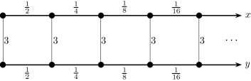
Figure 4: In this example there is no geodesic connecting the boundary points $x,y$ in $|$G$|_{\ell}$.

However, $|$G$|_{\ell}$ is always a geodesic metric space if it is compact:

Theorem 4.2.

If $|$G$|_{\ell}$ is compact then it is a geodesic metric space.

Proof.

It is an easy and well-known fact that a complete metric space is geodesic if it has “midpoints”, that is, if for any two points $x,y$ in the space there is a point $z$ so that $d(x,z)=d(z,y)=\frac{1}{2}d(x,y)$ holds. Let us show that $|$G$|_{\ell}$ does have midpoints if it is compact.

Pick $x,y\in|$G$|_{\ell}$, and let $h:=d_{\ell}(x,y)$. Choose a sequence $(P_{i})_{i\in\mathbb{N}}$ of finite paths in $G\$such that if $x_{i},y_{i}$ are the endvertices of $P_{i}$ then the sequence $(x_{i})_{i\in\mathbb{N}}$ converges to $x$, the sequence $(y_{i})_{i\in\mathbb{N}}$ converges to $y$, and $\lim\ell(P_{i})=h$; such a sequence $(P_{i})_{i\in\mathbb{N}}$ exists by the definition of $|$G$|_{\ell}$. Now for every $i$, consider $P_{i}$ as a topological path in the 1-complex $G$, and let $p_{i}$ be the midpoint of $P_{i}$, that is, the point on $P_{i}$ satisfying $\ell(x_{i}P_{i}p_{i})=\ell(p_{i}P_{i}y_{i})$. As by our assumption $|$G$|_{\ell}$ is compact, the sequence $(p_{i})_{i\in\mathbb{N}}$ has an accumulation point $z$, and it is easy to check that $d_{\ell}(x,z)=d_{\ell}(z,y)=\frac{1}{2}d(x,y)$ as desired. ∎

Next, we are going to prove two results that are needed in [23] but might be of independent interest.

For the following two lemmas suppose $G\$is countable, fix an enumeration $e_{1},e_{2},\ldots$ of $E(G)$, and let $E_{n}:=\{e_{1},\ldots,e_{n}\}$. Moreover, let $\mathaccent 28695{e}_{n}$ denote the set of inner points of the edge $e_{n}$, and let $\mathaccent 28695{E}_{n}:=\{\mathaccent 28695{e}_{1},\ldots,\mathaccent 28695{e}_{n}\}$.

Lemma 4.3.

Let $C$ be a circle or arc in $|$G$|_{\ell}$ such that $E(C)$ is dense in $C$. Then, for every $\epsilon\in\mathbb{R}_{+}$ there is an $n\in\mathbb{N}$ such that for every subarc of $C$ in $|$G$|_{\ell}\backslash\mathaccent 28695{E}_{n}$ connecting two vertices $v,w$ we have $d_{\ell}(v,w)<\epsilon$.

Proof.

We will only consider the case when $C$ is an arc; the case when $C$ is a circle is similar. Suppose, on the contrary, there is an $\epsilon$ such that for every $n\in\mathbb{N}$ there is a subarc $R_{n}$ of $C$ in $|$G$|_{\ell}\backslash\mathaccent 28695{E}_{n}$ the endvertices of which have distance at least $\epsilon$. Let $x_{n},y_{n}$ be the first and last vertex of $R_{n}$ respectively along $C$.

As $C$ is compact, the sequence $(x_{i})_{i\in\mathbb{N}}$ has a convergent subsequence $(x_{i})_{i\in I}$ with limit $x$ say, and the corresponding subsequence $(y_{i})_{i\in I}$ of $(y_{i})_{i\in\mathbb{N}}$ also has a converging subsequence $(y_{i})_{i\in J}$, $J\subseteq I$, with limit $y$ say. Since $d_{\ell}(x_{i},y_{i})\geq\epsilon$ we have $d_{\ell}(x,y)\geq\epsilon$, in particular $x\neq y$. Note that $C$ must contain the points $x,y$ because it is closed. But as $E(C)$ is dense in $C$, $xCy$ must meet some edge $e_{n}$ at an inner point $z$ say. It is easy to see that if $m$ is large enough then $x_{m}$ and $y_{m}$ lie in distinct components of $C\backslash\{z\}$. Thus for such an $m$ the subarc $R_{m}=x_{m}Cy_{m}$ contains $z$, and as we can choose $m$ to be larger than $n$ this contradicts the fact that $R_{m}$ avoids $\mathaccent 28695{e}_{n}$. ∎

Lemma 4.4.

If $\sum_{e\in E(G)}\ell(e)<\infty$ then for every circle or arc $C$ in $|$G$|_{\ell}$ we have $\ell(C)=\sum_{e\in E(C)}\ell(e)$.

Before proving this, let us see an example showing that the requirement $\sum_{e\in E(G)}\ell(e)<\infty$ in Lemma 4.4 is necessary, since without it $\ell(C)$ might be strictly greater than $\sum_{e\in E(C)}\ell(e)$ even if $E(C)$ is dense in $C$. In fact, this situation can occur even if $|$G$|_{\ell}\approx ETOP(G)$ —which is always the case if $\sum_{e\in E(G)}\ell(e)<\infty$ by Lemma 3.1. The existence of a circle $C$ in $|$G$|_{\ell}$ such that $E(C)$ is dense in $C$ but still $\ell(C)>\sum_{e\in E(C)}\ell(e)$ might look surprising at first glance, but perhaps less so bearing in mind that it is possible to construct a dense set of non-trivial subintervals of the real unit interval of arbitrarily small total length (e.g. imitating the construction of the Cantor set but removing shorter intervals).

Example 4.5.

Let $G\$be the graph of Figure 5, which is the same as the graph of Figure 1, and let every thin edge in the $i$-th level have length $c2^{-i}$ for some fixed $c\in\mathbb{R}_{>0}$ (in this example we chose $c=1$). Moreover, assign lengths to the thick edges in such a way that the sum $s$ of the lengths of all thick edges is finite ($s=1\frac{1}{2}$ in this example). Here we have, as an exception, allowed some edges to have length 0, but this can be avoided by contracting those edges. It is not hard to check that for this assignment $\ell$ we have $|$G$|_{\ell}\approx|G|$. Furthermore, it is not hard to check that the length of the wild circle $W$ is (at least) $s+c$, which is greater than $\sum_{e\in E(W)}\ell(e)=s$ (in this example, the length of the outer double ray $L$ is 1 and the length of $W\backslash L$ is $1\frac{1}{2}$). To see this, note for example that the two ends of the outer double ray $L$ have distance $\min(c,\ell(L))$, since every finite path $P$ connecting the leftmost ray to the rightmost one has length at least $c$ (use induction on the highest level that $P$ meets).

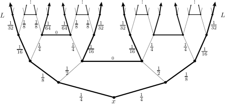
Figure 5: The length of the wild circle $W$ here is greater than the sum of the lengths of the edges in it.

We now proceed to the proof of Lemma 4.4.

Proof of Lemma 4.4.

By Theorem 3.1 we have $|$G$|_{\ell}\approx ETOP(G)$, and this easily implies that $E(C)$ is dense in $C$. By the definition of $\ell(C)$ it suffices to show that

$$d_{\ell}(x,y)\leq\sum_{e\in E(xCy)}\ell(e)$$ (3)

holds for every pair $x,y$ of points on $C$. To show that (3) holds, we will construct a sequence $(P_{i})_{i\in\mathbb{N}}$ of finite paths in $G$ such that the endpoints $x_{i},y_{i}$ of $P_{i}$ give rise to sequences converging to $x,y$ respectively, and for the sequence $\delta_{i}:=\sum_{e\in E(P_{i})\setminus E(xCy)}\ell(e)$ we have $\lim\delta_{i}=0$. This would easily imply $d_{\ell}(x,y)\leq\sum_{e\in E(xCy)}\ell(e)$ by the definition of $d_{\ell}$.

To begin with, pick an $r_{0}\in\mathbb{N}$ and let $P_{0}$ be any path in $G$. Then, for every $i=1,2,\ldots$, pick an $r_{i}>r_{i-1}$ large enough that the distance (in $|$G$|_{\ell}$) between the endvertices of any subarc of $xCy$ in $|$G$|_{\ell}\backslash\mathaccent 28695{E}_{r_{i}}$ is less than the length $h_{i-1}$ of the shortest edge in $\bigcup_{j<i}P_{j}$; such an $r_{i}$ exists by Lemma 4.3.

In order to define $P_{i}$, let $x_{i}$ be the first vertex of $xCy$ incident with $E_{r_{i}}$ and let $y_{i}$ be the last vertex of $xCy$ incident with $E_{r_{i}}$; such vertices exist because $xCy$ is a topological path and there are only finitely many vertices incident with $E_{r_{i}}$. Since $E(C)$ is dense in $C$, and since $\lim r_{i}=\infty$, it is easy to see that $x_{i}$ converges to $x$ and $y_{i}$ converges to $y$. Now for every maximal subarc $A$ of $x_{i}Cy_{i}$ in $|$G$|_{\ell}\backslash\mathaccent 28695{E}_{r_{i}}$ choose a finite $w$–$v$ path $P_{A}$, where $w,v$ are the endpoints of $A$, such that $\ell(P_{A})<h_{i-1}$; such a path $P_{A}$ exists since by the choice of $r_{i}$ we have $d_{\ell}(w,v)<h_{i-1}$. Then, replace $A$ in $x_{i}Cy_{i}$ by the path $P_{A}$. Note that there are only finitely many such arcs $A$ as $E_{r_{i}}$ is finite. Performing this replacement for every such subarc $A$ we obtain a (finite) $x_{i}$-$y_{i}$ walk $P^{\prime}_{i}$; let $P_{i}$ be an $x_{i}$-$y_{i}$ path with edges in $P^{\prime}_{i}$.

By the choice of the paths $P_{A}$ we obtain that the edge-sets $E(P_{i})\setminus E(xCy)$ are pairwise disjoint, and as $\sum_{e\in E(G)}\ell(e)<\infty$ this implies $\lim\delta_{i}=0$ as required. ∎

For $\omega\in\Omega(G)$ denote by $\left<\omega\right>_{\ell}$ the set

$$\{x\in\partial^{\ell}G\mid\text{ there is an $\omega$-ray that converges to $x$ in $|$G$|_{\ell}$}\}.$$

(Recall that $\partial^{\ell}G$ is the set of boundary points of $|$G$|_{\ell}$.) For the rest of this section assume $G\$to be locally finite. Note that by Lemma 4.1 every point in $\partial^{\ell}G$ lies in $\left<\omega\right>_{\ell}$ for some end $\omega$. It has been proved that if $G\$is a hyperbolic graph and $|$G$|_{\ell}$ is its hyperbolic compactification (see Section 3.2), then $\left<\omega\right>_{\ell}$ is a connected subspace of $|$G$|_{\ell}$ for every $\omega\in\Omega(G)$ [27, Chapter 7 Proposition 17]. The following proposition generalises this fact to an arbitrary compact $|$G$|_{\ell}$.

Theorem 4.6.

If $G\$is locally finite and $|$G$|_{\ell}$ is compact then $\left<\omega\right>_{\ell}$ is connected for every $\omega\in\Omega$.

Before proving this, let us make a couple of related remarks. If $\omega,\psi$ are distinct ends of $G$, then there is a finite edge set $S$ that separates them. But then, for every assignment $\ell:E(G)\to\mathbb{R}_{>0}$, and any choice of elements $x\in\left<\omega\right>_{\ell},y\in\left<\psi\right>_{\ell}$, we have $d_{\ell}(x,y)\geq r$ where $r$ is the minimum length of an edge in $S$. This implies, firstly, that $\left<\omega\right>_{\ell}$ is a closed subspace of $\partial^{\ell}G$, and thus of $|$G$|_{\ell}$, for every end $\omega$, and secondly, that every two points $x,y$ as above lie in distinct components of $\partial^{\ell}G$. Thus, in the case that $|$G$|_{\ell}$ is compact, Theorem 4.6 characterises the components of $\partial^{\ell}G$: they are precisely the sets of the form $\left<\omega\right>_{\ell}$.

Proof of Theorem 4.6..

Suppose, on the contrary, that $|$G$|_{\ell}$ is compact but $\left<\omega\right>_{\ell}$ disconnected. Then, there is a bipartition $\{O_{1},O_{2}\}$ of $\left<\omega\right>_{\ell}$ where both $O_{1},O_{2}$ meet $\left<\omega\right>_{\ell}$ and both are clopen in the subspace topology of $\left<\omega\right>_{\ell}$. As $\left<\omega\right>_{\ell}$ is a closed subspace of $|$G$|_{\ell}$ it must be compact, and so there is a lower bound $r>0$ such that for every $x\in O_{1}$ and $y\in O_{2}$ we have $d_{\ell}(x,y)>r$. Let $U_{1}:=\bigcup_{x\in O_{1}}B_{x}(\frac{r}{2})$ and $U_{2}:=\bigcup_{y\in O_{2}}B_{y}(\frac{r}{2})$ where the sets of the form $B_{x}(\frac{r}{2})$ are open balls in $|$G$|_{\ell}$; note that $U_{1},U_{2}$ are disjoint open sets of $|$G$|_{\ell}$.

Pick a point $x\in O_{1}$ and a point $y\in O_{2}$. Moreover, pick $\omega$-rays $R,T$ in $G$ converging (in $|$G$|_{\ell}$) to $x,y$ respectively. Since $R$ and $T$ are vertex-equivalent, there is an infinite set $\mathcal{P}$ of pairwise disjoint $R$–$T$ paths.

Note that $U_{1}$ contains a tail of $R$ and $U_{2}$ contains a tail of $T$. If $U_{1}\cup U_{2}$ contains infinitely many of the paths in $\mathcal{P}$, then we can combine $R,T$, and one of those paths, to construct a double ray $D$ contained in $U_{1}\cup U_{2}$. However, the union of $D$ with $\{x,y\}$ is an $x$–$y$ arc in $|$G$|_{\ell}$, and this contradicts the choice of $U_{1},U_{2}$ as arcs are connected spaces.

Thus the subset $\mathcal{P}^{\prime}\subseteq\mathcal{P}$ of paths $P$ that contain a point $q_{P}$ not in $U_{1}\cup U_{2}$ is infinite. Let $p$ be an accumulation point of $\{q_{P}\mid P\in\mathcal{P}^{\prime}\}$, and note that $p\not\in U_{1}\cup U_{2}$. Easily, $p\in\partial^{\ell}G$. Let $(p_{i})_{i\in\mathbb{N}}$ be a sequence of elements of $\{q_{P}\mid P\in\mathcal{P}^{\prime}\}$ converging to $p$. We may assume, without loss of generality, that every $p_{i}$ is a vertex, for if it is an inner point of the edge $e=uv$, then we can subdivide $e$ into two edges one of which has length equal to the length of the $u$-$p_{i}$ half-edge and the other has length equal to the length of the $p_{i}$-$v$ half-edge. We can now apply Lemma 4.1 to $(p_{i})_{i\in\mathbb{N}}$, and as $G\$is locally finite we obtain a comb $K$ that contains infinitely many of the $p_{i}$ and converges to $p$. On the other hand, the paths in $\mathcal{P}$ combined with the ray $R$ yield another comb, whose spine is $R$, containing infinitely many of the $p_{i}$. Combining these two combs it is easy to see that the spine of $K$ is vertex-equivalent to $R$, which means that $p\in\left<\omega\right>_{\ell}$; this however contradicts the fact that $p\not\in U_{1}\cup U_{2}$.

∎

Having seen Theorem 4.6, it is natural to wonder whether $\left<\omega\right>_{\ell}$ is always path-connected in case $|$G$|_{\ell}$ is compact. As we shall see, this is not the case.

Gromov [28] remarked that for every compact metric space $X$ there is a hyperbolic graph whose hyperbolic boundary is isometric to $X$; thus by Lemma 3.3 every compact space can be obtained as the $\ell\text{-}TOP$-boundary of some locally finite graph. Our next result strengthens this fact by relaxing the requirement that $X$ be compact.

Theorem 4.7.

Given a metric space $(X,d_{X})$, there is a connected locally finite graph $G\$and $\ell:E(G)\to\mathbb{R}_{>0}$ such that $\partial^{\ell}G$ is isometric to $X$ if and only if $X$ is complete and separable.

Proof.

For the backward implication, let $U=\{u_{1},u_{2},\ldots\}$ be a countable dense subset of $X$. To define $G$, let its vertex set $V$ consist of vertices $z^{n}_{u}$, one for each ${n\in\mathbb{N}}$ and $u\in U$. The edge set of $G\$is constructed as follows. For every $u\in U$ and every ${n\in\mathbb{N}}$, connect $z^{n}_{u}$ to $z^{n+1}_{u}$ by an edge $e$, and let $\ell(e):=2^{-n}$. Moreover, for every ${n\in\mathbb{N}}$ and every pair $u_{i},u_{j}\in U$ such that $i,j\leq n$, connect $z^{n}_{u_{i}}$ to $z^{n}_{u_{j}}$ by an edge $e$, and let $\ell(e):=d_{X}(u_{i},u_{j})$.

We now define the required isometry $f:X\to\partial^{\ell}G$. For every $u\in U$, let $f(u):=\lim_{n}z^{n}_{u}$. By the choice of $\ell$, it follows easily that $d_{\ell}(f(u),f(u^{\prime}))\leq d_{X}(u,u^{\prime})$ for every $u,u^{\prime}\in U$. Applying the triangle inequality for $d_{X}$ it is also straightforward to check that $d_{\ell}(f(u),f(u^{\prime}))\geq d_{X}(u,u^{\prime})$. Thus we obtain

$$d_{\ell}(f(u),f(u^{\prime}))=d_{X}(u,u^{\prime}) u,u^{\prime}\in U$$ for every  (4)

as desired. For every other point $x\in X$, let $(x_{i})_{i\in\mathbb{N}}$ be a Cauchy sequence of points in $U$ converging to $x$. Note that by (4) the sequence $(f(x_{i}))$ is also Cauchy. Thus we may define $f(x):=\lim f(x_{i})$. It is an easy consequence of (4) and the definition of $f$ that $f$ is distance preserving.

To see that $f$ is surjective, let $(z^{n_{i}}_{u_{m_{i}}})_{i\in\mathbb{N}}$ be a Cauchy sequence (in $|$G$|_{\ell}$) of vertices of $G$ converging to a point $\psi\in\partial^{\ell}G$. By the construction of $G\$and $\ell$, we have $d_{X}(u_{m_{i}},u_{m_{j}})\leq d_{\ell}(z^{n_{i}}_{u_{m_{i}}},z^{n_{j}}_{u_{m_{j}}})$ for every $i,j$, which implies that the sequence $(u_{m_{i}})_{i\in\mathbb{N}}$ of $X$ is also Cauchy. Moreover, since $(z^{n_{i}}_{u_{m_{i}}})_{i\in\mathbb{N}}$ converges to $\partial^{\ell}G$ we have $\lim_{i}n_{i}=\infty$; thus $(z^{n_{i}}_{u_{m_{i}}})_{i\in\mathbb{N}}$ is equivalent to the sequence $(f(u_{m_{i}}))_{i\in\mathbb{N}}$. This, and the definition of $f$, implies that $f(\lim u_{m_{i}})=\psi$. We have proved that $f$ is surjective, which means that it is indeed an isometry.

For the forward implication, let $G\$be a countable graph and fix $\ell:E(G)\to\mathbb{R}_{>0}$. Then $\partial^{\ell}G$ is clearly complete. To show that it is separable, it suffices to show that it is second countable, and a countable basis for $\partial^{\ell}G$ is $\mathcal{U}:=\{\partial^{\ell}G\cap B_{r}(x)\mid x\in V(G),r\in\mathbb{Q}\}$ where $B_{r}(x)$ is the open ball of radius $r$ and center $x$.

∎

If the metric space $X$ in Theorem 4.7 is compact, then it is possible to modify the proof so that $|$G$|_{\ell}$ is also compact; for example, by using Gromov’s aforementioned construction and Theorem 3.3. Since there are compact spaces that are connected but not path-connected, this, and Theorem 4.6, implies that $\left<\omega\right>_{\ell}$ can be non-path-connected for some end $\omega$ even if it is compact, although it must be connected.

5 Homology and Cycle space

5.1 Introduction

In this section we are going to describe a new homology $H_{\ell}(X)$ defined on an arbitrary metric space $X$. It is proved in [22] that $H_{\ell}(X)$ coincides, in dimension 1, with the topological cycle space $\mathcal{C}(G)$ discussed in Section 1.3 if applied to the metric space $|$G$|_{\ell}$ for the right function $\ell$, and that $H_{\ell}(X)$ extends properties of $\mathcal{C}(G)$ to every compact metric space $X$. We will discuss, in particular, how $H_{\ell}$ can be used to extend results about the topological cycle space of a locally finite graph to non-locally-finite graphs.

In order to define $\mathcal{C}(G)$ for a locally finite graph $G$, we call a set of edges $D\subseteq E(G)$ a circuit, if there is a topological circle $C$ in $|G|$ that traverses every edge in $D$ but no edge outside $D$. Then, let $\mathcal{C}(G)$ be the vector space over $\mathbb{Z}_{2}$ consisting of those subsets $F$ of $E(G)$ such that $F$ can be written as the sum of a possibly infinite family of circuits; such a sum is well-defined, and allowed, if and only if the family is thin, that is, no edge appears in infinitely many summands: the sum of such a family $\mathcal{F}$ is by definition the set of edges that appear in an odd number of members of $\mathcal{F}$.

The study of $\mathcal{C}(G)$ has been a very active field lately [12], but non-locally-finite graphs have received little attention. One reason for this is the fact that $|G|$ can be generalised to non-locally-finite graphs in several ways (see Section 3.3), all having advantages and disadvantages, and it was not clear which of them is the right topology on which the definition of $\mathcal{C}$ should be based. Let me illustrate this by an example. In the graph of Figure 6 (ignore the indicated edge lengths for the time being), let $\mathcal{F}$ be the family of all triangles incident with $x$. Note that $\mathcal{F}$ is a thin family, and its sum comprises the edge $xz$ and all edges of the horizontal ray. Now such an edge set can only be considered to be a circuit if the topology chosen identifies $x$ with the end $\omega$ of the graph. Similarly, the vertex $y$ also has to be identified with $\omega$, and thus also with $x$, if such sums are to be allowed. So we either have to forbid these infinite sums, or content ourselves with a topology that changes the structure of the graph by identifying vertices. Both approaches have been considered [17, 18], but none was pursued very far.

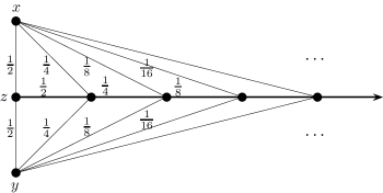
Figure 6: A simple non-locally-finite graph.

Let me now argue that with $|$G$|_{\ell}$ we might be able to overcome this dilemma: our aim is to define, for a graph $G$ and $\ell:E(G)\to\mathbb{R}_{>0}$, a cycle space $\mathcal{C}_{\ell}$ based on circles in the topology $|$G$|_{\ell}$, and prove results that hold for every $\ell$ and generalise the properties of the cycle space of a finite graph. As we shall see, this would allow us to postpone the decision of whether to identify vertices or forbid some infinite sums until we have a certain application in mind. See also the remark at the end of Section 3.3.

Suppose for example that we allow in $\mathcal{C}_{\ell}$ precisely those sums of families $\{F_{i}\}_{i\in I}$ of circuits, that is, edge sets of circles in $|$G$|_{\ell}$, that have finite total length, i.e. satisfy $\sum_{i}\sum_{e\in F_{i}}\ell(e)<\infty$. Firstly, note that such a family is always thin, since if an edge $e$ lies in infinitely many $F_{i}$ then the total length of $\{F_{i}\}_{i\in I}$ will be infinite. We will now consider two special assignments $\ell_{1},\ell_{2}$ of lengths to the edges of the graph $G\$of Figure 6, and see how $\mathcal{C}_{\ell}$ behaves in these two interesting cases.

Let $\ell_{1}$ be an assignment of lengths as shown in Figure 6. Then, the family of all triangles of $G\$has finite total length, so their sum lies in $\mathcal{C}_{\ell}$. This sum is the edge set $\{xz,zy\}$. On the other hand, $x$ and $y$ have distance $d_{\ell_{1}}(x,y)=0$ in this case, which means that $x$ and $y$ are identified in $|$G$|_{\ell}$ and $\{xz,zy\}$ is indeed a circuit.

For the second case, let $\ell_{2}(e)=1$ for every $e\in E(G)$. Then, $x$ and $y$ are not identified, so $\{xz,zy\}$ is not a circuit, but it is also not in $\mathcal{C}_{\ell}$, since every infinite family of circuits has infinite total length.

The interested reader will try other assignments of edge lengths for this graph and convince himself that $\mathcal{C}_{\ell}$ always behaves well in the sense that for any $\ell:E(G)\to\mathbb{R}_{>0}$ any element of $\mathcal{C}_{\ell}$ can be written as the sum of a family of pairwise edge disjoint circuits.

Although $\mathcal{C}_{\ell}$ performs well in simple cases like Figure 6, it is a rather naive concept, since in general, even if $G\$is locally finite, there can be arcs and circles in $|$G$|_{\ell}$ that contain no vertex and no edge of $G$; this can be the case for example when $|$G$|_{\ell}$ is the hyperbolic compactification of $G$, see Section 3.2. Thus circuits do not describe their circles accurately enough. To make matters worse, even if we decide to disregard those circles that have subarcs contained in the boundary, and consider only those circles $C$ for which $E(C)$ is dense in $C$ we will not obtain a satisfactory cycle space as we shall see in the next section.

For these reasons, we will follow an approach combining singular homology with the above ideas. This will lead us, in Section 5.3, to the homology $H_{\ell}$ that apart for graphs endowed with $\ell\text{-}TOP$ can be defined for arbitrary metric spaces.

5.2 Failure of the edge-set approach

Given a graph $G\$and $\ell:E(G)\to\mathbb{R}_{>0}$, let us call a (topological) circle $C$ in $|$G$|_{\ell}$ proper if $E(C)$ is dense in $C$. Following up the above discussion, let us define $\mathcal{C}_{\ell}$ to be the vector space over $\mathbb{Z}_{2}$ consisting of those subsets $F$ of $E(G)$ such that $F$ can be written as the sum of a (thin) family $\{F_{i}\}_{i\in I}$ of circuits of proper topological circles in $|$G$|_{\ell}$ such that $\sum_{i}\sum_{e\in F_{i}}\ell(e)<\infty$. Although $\mathcal{C}_{\ell}$ behaves well with respect to the graph in Figure 6, it turns out that it is not a good concept: we will now construct an example in which $\mathcal{C}_{\ell}$ has an element that contains no circuit. The reader who is already convinced that circuits cannot describe the circles in $|$G$|_{\ell}$ accurately enough could skip to Section 5.3, however it is advisable to go through the following example anyway, as it will facilitate the understanding of the homology $H_{\ell}$ introduced there.

Example 5.1.

The graph $G\$we are going to construct contains a proper circle $C_{0}$ like in Example 4.5 (Figure 5), the length of which is larger than the sum of the lengths of its edges. Moreover, it is possible to replace each edge of $C_{0}$ by an arc which also has a length larger than the sum of the lengths of its edges to obtain a new proper circle $C_{1}$. We then replace each edge of $C_{1}$ by such an arc to obtain the proper circle $C_{2}$, and so on. The proper circles $C_{i}$ will have lengths that grow slightly  with $i$, but the proportion of that length accounted for by the edges will tend to 0 as $i$ grows to infinity. Moreover, the $C_{i}$ will converge  to a circle $C$ containing no edges at all. This is the point where $\mathcal{C}_{\ell}(G)$ will break down: we will define a family $(F_{i})$ of sums of circuits such that for every $j\in\mathbb{N}$ the edge set $\sum_{i\leq j}F_{j}$ is the circuit of $C_{j}$, but $\sum_{i\in\mathbb{N}}F_{j}=0$. Thus $(F_{i})$ tends to describe the circles $C_{i}$, but its “limit” fails to describe their limit $C$, and we will exploit this fact to construct pathological elements of $\mathcal{C}_{\ell}(G)$.

We will perform the construction of both the underlying graph $G\$and the required family recursively (and simultaneously), in $\omega$ steps. After each step $i$, we will have defined the graph $G_{i}$ and the edge-sets $F_{0},\ldots F_{i}$, with $F_{j}\subseteq E(G_{j})$, so that $\sum_{0\leq j\leq i}F_{j}$ is the circuit of a proper circle $C_{i}$ such that  $\ell(E(C_{i}))\leq 2^{-i}$. The graph in which the pathological elements of $\mathcal{C}_{\ell}$(G) live is $G:=\bigcup G_{i}$. In each step we will specify the lengths of the newly added edges, and we will choose them in such a way that for every $i$ and every two vertices $x,y\in G_{i}$ the distance $d_{\ell}(x,y)$ is not influenced by edges added after step $i$; in other words, no $x$–$y$ path in $G$ has a length less than the distance between $x$ and $y$ in $G_{i}$. This implies that any circle of $G_{i}$ is also a circle of $G$.

Formally, for step $0$, let $G_{0}$ be the graph in Example 4.5 (with edge lengths as in that example), let $C_{0}$ be the thick, “wild” circle there, and let $F_{0}=E(C_{0})$ be its circuit. Then, for $i=1,2,\ldots$, suppose we have already performed step $i$ so that it satisfies the above requirements. In step $i+1$, for every edge $e=vw$ of $C_{i}$, take a copy $H_{e}$ of the graph of Example 4.5, and let $W_{e}$ denote the circle of $H_{e}$ corresponding to the thick circle $W$ in Example 4.5. Recall that $\ell(W)=2\frac{1}{2}$ but $\sum_{e\in E(W)}\ell(e)=1\frac{1}{2}$. The vertex of $H_{e}$ corresponding to the vertex $x$ in Figure 5 divides the outer double ray $L_{e}$ into two rays $R,S$; now join, for every $j\in\mathbb{N}$, the $j$th vertex of $R$ to the endpoint $v$ of $e$ by an edge of length $\ell(e)/2^{j-1}$ and also join the $j$th vertex of $S$ to the other endpoint $w$ of $e$ by an edge of length $\ell(e)/2^{j-1}$; see Figure 7. Note that $v$ and $w$ have infinite degree now. Later we will see how the construction can be modified to obtain a locally finite graph with similar properties.

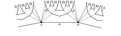
Figure 7: Joining the graphs $H_{e}$ to $G_{i}$ to obtain $G_{i+1}$.

Now change the lengths of the edges of $H_{e}$ as follows. Scale the lengths of the edges in $E(H_{e})$ down in such a way that the distance of the endpoints of $W_{e}\backslash L_{e}$ is $\ell(e)$ and so that

$$\sum_{f\in E(W_{e})\backslash E(L_{e})}\ell(f)=\ell(e)/2$$. (5)

Such a choice of edge-lengths is possible since in Example 4.5 we were allowed to choose $s$ and $c$ independently from each other.

Note that by the choice of the lengths of the newly attached edges, no $v$–$w$ path going through $H_{e}$ has a length less than $\ell(e)$. Moreover, since the lengths of the newly added edges converge to 0, the distance between $v$ and the end of the ray $R$ is 0, and the distance between $w$ and the end of the ray $S$ is also 0. Thus the union of $e$ with the arc $W_{e}\backslash L_{e}$ is a topological circle $C_{e}$.

Having performed this operation for every edge $e$ of $C_{i}$ we obtain the new graph $G_{i+1}$. We now let $F_{i+1}:=\sum_{e\in E(C_{i})}E(C_{e})$. Moreover, let $C_{i+1}$ be the topological circle in $|G_{i+1}|_{\ell}$ obtained from $C_{i}$ by replacing each edge $e\in E(C_{i})$ by the arc $C_{e}\backslash\mathaccent 28695{e}=W_{e}\backslash L_{e}$. This completes step $i+1$. Note that

$$E(C_{i+1})=E(C_{i})+F_{i+1}$$, (6)

thus assuming, inductively, that $\sum_{j\leq i}F_{j}=E(C_{i})$, we obtain $\sum_{j\leq i+1}F_{j}=E(C_{i+1})$.

Let $\ell_{i}:=\sum_{e\in F_{i}}\ell(e)$. As the circles $C_{i}$ and $C_{i+1}$ are edge-disjoint, (6) implies $F_{i}=E(C_{i})\cup E(C_{i+1})$, and thus

$$\ell_{i}=\sum_{e\in E(C_{i+1})}\ell(e)+\sum_{e\in E(C_{i})}\ell(e).$$

By (5) and the definition of $C_{i+1}$ we obtain $\sum_{e\in E(C_{i+1})}\ell(e)=\frac{1}{2}\sum_{e\in E(C_{i})}\ell(e)$. Plugging this inequality into the above equation twice (for two subsequent values of $i$), yields $\ell_{i}=\frac{\ell_{i-1}}{2}$. Thus the family $(F_{i})_{i\in\mathbb{N}}$ does have finite total length.

Now as $F_{i}=E(C_{i})\cup E(C_{i+1})$ and the circles $C_{i}$ and $C_{i+1}$ are edge-disjoint, every edge in $\bigcup F_{i}$ appears in precisely two members of $(F_{i})$ and thus $\sum_{i\in\mathbb{N}}F_{i}=\emptyset$. We can now slightly modify the family $(F_{i})$ to obtain a new finite-length family $(F^{\prime}_{i})$ of circuits of proper circles in $G=\bigcup G_{i}$ the sum of which is a single edge: pick an edge $f$ of $C_{0}$, remove from $F_{1}$ the circuit of $C_{f}$, then remove from $F_{2}$ all circuits of circles $C_{e}$ corresponding to edges $e$ that lie in $C_{f}$, and so on. For the resulting family $(F^{\prime}_{i})$ we then have $\sum_{i\in\mathbb{N}}F^{\prime}_{i}=\{f\}$, and as $(F^{\prime}_{i})$ has finite total length the singleton $\{f\}$ is an element of $\mathcal{C}_{\ell}$, and in fact a pathological one as the endvertices of $f$ are distinct points in $|$G$|_{\ell}$.

Transforming this example to a locally finite one with the same properties is easy. The intuitive idea is to replace each vertex of infinite degree of $G$ by an end and its incident edges by double rays “connecting” the corresponding ends. More precisely, let $H$ be a copy of the graph of Figure 5, and subdivide every edge $e=uv$ of $H$ into two edges $ux_{e},x_{e}v$ to obtain the graph $H^{\prime}$; assign lengths to the new edges so that $\ell(ux_{e})+\ell(x_{e}v)=\ell(uv)$. Then, for every vertex $u\in V(H^{\prime})\cap(V(H)\backslash V(L))$, replace each (subdivided) edge $ux_{e}$ incident with $u$ by a ray starting at $x_{e}$ and having total length $\ell(ux_{e})$, and make all these rays converge to the same point by joining them by infinitely many new edges with lengths tending to zero. Denote the end containing these (now equivalent) rays by $\omega_{u}$, and note that the lengths of the newly added edges can be chosen so that the distance between any two such ends $\omega_{u},\omega_{v}$ of the new graph equals the distance between $u$ and $v$ in $H$. This gives rise to a new graph $H^{\prime\prime}$, and we may use $H^{\prime\prime}$ instead of $H$ as a building block in the above construction of $G$, to obtain a locally finite graph similar to $G$; instead of the attaching operation of Figure 7 we would now use an operation as indicated in Figure 8 (and instead of attaching, at step $i+1$, a new copy of $H^{\prime\prime}$ for each edge of $C_{i}$ we will attach a new copy of $H^{\prime\prime}$ for each double ray in $C_{i}$).

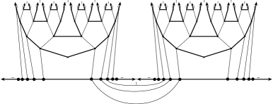
Figure 8: Modifying the construction of $G\$to make it locally finite.

Example 5.1 and our previous discussion show that the edge-sets of circles do not reflect the structure of a graph accurately enough, so we will take another tack: in the following section we are going to study circles from the point of view of singular homology.

5.3 The singular-homology point of view

The topological cycle space $\mathcal{C}$ of a locally finite graph $G$, discussed in Sections 1.3 and 5.1, bears some similarity to the first singular homology group $H_{1}$ of $|G|$, as both are based on circles, i.e. closed 1-simplices, in $|G|$. Diestel and Sprüssel [19] investigated the precise relationship between $\mathcal{C}(G)$ and $H_{1}(|G|)$, and found out that they are not the same: they defined a canonical mapping $f:H_{1}(|G|)\to\mathcal{C}(G)$ that assigns to every class $c\in H_{1}(|G|)$ the set of edges traversed by one (and thus, as they prove, by every) representative of $c$ an odd number of times —assuming both $\mathcal{C}$ and $H_{1}$ are defined over the group $\mathbb{Z}_{2}$— and showed that $f$ is a group homomorphism that is surjective, but not necessarily injective. Example 5.2 below shows their construction of a non-zero element of $H_{1}(|G|)$ that $f$ maps to the zero element of $\mathcal{C}(G)$.

Example 5.2.

The space $X$ (solid lines) depicted in Figure 9 can be thought of as either the Freudenthal compactification $|G|$ of the infinite ladder $G$, or as a subset of the euclidean plane; note that the two spaces are homeomorphic, since the set of vertices converges to a single limit point in both of them.

Let $\sigma$ be the 1-simplex indicated by the dashed curve. This simplex starts and ends at the upper-left vertex, traverses every horizontal edge twice in each direction, and traverses every vertical edge once in each direction. Thus it is mapped to the zero element of $\mathcal{C}(G)$ by the mapping $f$. However, Diestel and Sprüssel [19] proved that $\sigma$ does not belong to the zero element of $H_{1}(|G|)$.

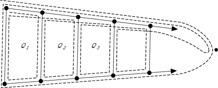
Figure 9: The 1-simplex of Diestel and Sprüssel. It traverses each edge the same number of times in each direction, but it is not null-homologous.

In what follows we are going to modify $H_{1}$ into a new homology group $H_{\ell}$ that does coincide with $\mathcal{C}$ if applied to $|G|$, and moreover generalises properties of $\mathcal{C}$ when applied to an arbitrary continuum. The main idea is to impose a pseudo-metric on $H_{1}$ and identify elements with each other if their distance is $0$. (Here we will constrain ourselves to dimension 1 for simplicity, but the construction can be carried out for any dimension, see [22].)

For this, let $X$ be a metric space and define an area-extension of $X$ to be a metric space $X^{\prime}$, in which $X$ is embedded by a fixed isometry $i:X\to X^{\prime}$, such that each component of $X^{\prime}\backslash i(X)$ is either a disc or a cylinder. The area of this extension is the sum of the areas of the components of $X^{\prime}\backslash i(X)$.

We now define a pseudo-metric $d_{1}$ on the first singular homology group $H_{1}(X)$ of $X$. Given two elements $[\phi],[\chi]$ of $H_{1}(X)$, where $\phi$ and $\chi$ are $1$-chains, let $d_{1}([\phi],[\chi])$ be the infimum of the areas of all area-extensions $X^{\prime}$ of $X$ such that $\phi$ and $\chi$ belong to the same element of $H_{1}(X^{\prime})$.

It follows easily by the definitions that $d_{1}$ satisfies the triangle inequality. However, $d_{1}$ is not a metric, since there may exist $c,f\in H_{1}$, $c\neq f$, with $d_{1}(c,f)=0$; indeed, for the class $c$ of the simplex of Example 5.2 we have $d_{1}(c,\mathbb{0})=0$, although $c$ is not the zero element $\mathbb{0}$ of $H_{1}$; to see that $d_{1}(c,\mathbb{0})=0$, let $Q_{j}$ be the $j$th 4-gon in the space $X$ of Example 5.2, and consider the area-extension $X^{i}$ of $X$ obtained by pasting to $X$ the plane discs bounded by all 4-gons $Q_{j}$ for $j>i$. Easily, $X$ is indeed isometrically embedded in $X^{i}$. It is straightforward to check that the simplex $\sigma$ of Example 5.2 is null-homologous in $X^{i}$. Moreover, the area of $X^{i}$ if finite for every $i$, and this area tends to 0 as $i$ grows to infinity. Thus by the definition of $d_{1}$, we have $d_{1}(c,\mathbb{0})=0$ as claimed.

Declaring $c,f\in H_{1}$ to be equivalent if $d_{1}(c,f)=0$ and taking the quotient with respect to this equivalence relation we obtain the group $H^{\prime}_{\ell}=H^{\prime}_{\ell}(X)$; the group operation on $H^{\prime}_{\ell}$ can be naturally defined for every $c,d\in H^{\prime}_{\ell}$ by letting $c+d$ be the equivalence class of $\alpha+\beta$ where $\alpha\in c$ and $\beta\in d$. To see that this sum is well defined, i.e. does not depend on the choice of $\alpha$ and $\beta$, note that the union of two area-extensions of $X$, of area at most $\epsilon$ each, is an area-extension of $X$ of area at most $2\epsilon$.

Now $d_{1}$ induces a distance function on $H^{\prime}_{\ell}$, which we will, with a slight abuse, still denote by $d_{1}$. It is not hard to prove that $d_{1}$ is now a metric on $H^{\prime}_{\ell}$; see [22] for details. We now define our desired group $H_{\ell}=H_{\ell}(X)$ to be the completion of the metric space $(H^{\prime}_{1},d)$. (The operation of $H_{\ell}$ is defined, for every $C,D\in H_{\ell}$, by $C+D:=\lim_{i}(c_{i}+d_{i})$ where $(c_{i})_{i\in\mathbb{N}}$ is a Cauchy sequence in $C$ and $(d_{i})_{i\in\mathbb{N}}$ is a Cauchy sequence in $D$.)

It can be proved that $\mathcal{C}(G)$, where $G\$is a locally finite graph, is a special case of $H_{\ell}$:

Theorem 5.3 ([22]).

If $\sum_{e\in E(G)}\ell(e)<\infty$ then $H_{\ell}(|$G$|_{\ell})$ is isomorphic to $\mathcal{C}(G)$.

(Recall that if $\sum_{e\in E(G)}\ell(e)<\infty$ then $|$G$|_{\ell}\approx|G|$ by Theorem 1.1.) The isomorphism of Theorem 5.3 is canonical, assigning to the class corresponding to a circle $C$ in $|$G$|_{\ell}$ the set of edges traversed by $C$.

The interested reader will check that $H_{\ell}$ also behaves well with respect to Example 5.1. The important observation is that for every $i$ there is an area-extension $X^{i}$ of the space $|$G$|_{\ell}$  in which all circles $C_{j}$ for $j>i$ become homologous to each other, and by the choice of the lengths of the circles $W_{e}$, the $X^{i}$ can be constructed so that the area of $X^{i}$ tends to 0 as $i$ grows to infinity.

Having seen Theorem 5.3, we could try to use $H_{\ell}$ to extend results about the cycle space of a finite or locally finite graph to other spaces, for example non-locally-finite graphs (recall our discussion in Section 5.1). But in order to be able to do so we would first have to interpret those results into a more “singular” language. In this and the next section we are going to see three examples of how this can be accomplished.

The main result of [22] is that $H_{\ell}$ extends the following fundamental property of $\mathcal{C}(G)$:

Lemma 5.4 ([13, Theorem 8.5.8]).

Every element of $\mathcal{C}(G)$ is a disjoint union of circuits.

Lemma 5.4 has found several applications in the study of $\mathcal{C}(G)$ [7, 16, 26] and elsewhere [24], and several proofs have been published [25]. The following theorem generalises Lemma 5.4 to $H_{\ell}(X)$ in case $X$ is a compact metric space.

Recall that an 1-cycle is a (finite) formal sum of 1-simplices that lies in the kernel of the boundary operator $\partial_{1}:C_{1}\to C_{0}$ ([30]). A representative of $C\in H_{\ell}$ is an infinite sequence $(z_{i})_{i\in\mathbb{N}}$ of $1$-cycles $z_{i}$ such that the sequence $(\overline{\sum_{j\leq i}z_{j}})_{i\in\mathbb{N}}$ is a Cauchy sequence in $C$, where $\overline{z}$ denotes the element of $H^{\prime}_{\ell}$ corresponding to the $1$-cycle $z$. (One can think of a representative as an “1-cycle” comprising infinitely many 1-simplices.) For an 1-cycle $z$ we define its length $\ell(z)$ to be the sum of the lengths of the simplices appearing in $z$ with a non-zero coefficient. Note that the coefficients of the 1-simplices in $z$ do not play any role in the definition of $\ell(z)$ as long as they are non-zero; in particular, $\ell(z)\geq 0$ for every $z$.

Theorem 5.5 ([22]).

For every compact metric space $X$ and $C\in H_{\ell}(X)$, there is a representative $(z_{i})_{i\in\mathbb{N}}$ of $C$ that minimizes $\sum_{i}\ell(z_{i})$ among all representatives of $C$. Moreover, $(z_{i})_{i\in\mathbb{N}}$ can be chosen so that each $z_{i}$ is a circlex.

(See Section 2.2 for the definition of circlex.)

Theorem 5.5 in conjunction with Theorem 5.3 imply in particular Lemma 5.4. Indeed, given a locally finite graph $G$, pick an assignment $\ell:E(G)\to\mathbb{R}_{>0}$ with $\sum_{e\in E(G)}\ell(e)<\infty$; now each element $C$ of $\mathcal{C}(G)$ corresponds, by Theorem 5.3, to an element $f(C)$ of $H_{\ell}(|$G$|_{\ell})=H_{\ell}(|G|)$ (where we applied Theorem 1.1). Applying Theorem 5.5 to $f(C)$ we obtain the representative $(z_{i})_{i\in\mathbb{N}}$ where each $z_{i}$ is a circlex. Note that no edge $e$ can be traversed by both $z_{i}$ and $z_{j}$ for $i\neq j$, for if this was a case then we could “glue” $z_{i}$ and $z_{j}$ together after removing the edge $e$ from both, to obtain a new representative $(z^{\prime}_{i})_{i\in\mathbb{N}}$ of $f(C)$ with $\sum_{i}\ell(z^{\prime}_{i})=\sum_{i}\ell(z_{i})-2\ell(e)$, contradicting the choice of $(z_{i})$. It follows that $\{E(z_{i})\mid{i\in\mathbb{N}}\}$ is a set of pairwise disjoint circuits whose union is $C$.

6 Geodetic circles and MacLane’s planarity criterion

A cycle in a graph $G\$is geodetic, if for every $x,y\in V(C)$ one of the two $x\text{--}y~{}paths$ in $C$ is a shortest $x\text{--}y~{}path$ also in the whole graph $G$. More generally, a circle $C$ in a metric space $(X,d)$ is geodetic, if for every $x,y\in C$ one of the two $x\text{--}y~{}arcs$ in $C$ has length $d(x,y)$. If $X$ is a finite graph then it is an easy, but interesting, fact that its geodetic circles generate its cycle space [26]. The following conjecture is an attempt to generalise this fact to an arbitrary continuum, or at least to an arbitrary compact $|$G$|_{\ell}$, using the homology group $H_{\ell}$ of Section 5.

For a set $U\subseteq H_{\ell}$, or $U\subseteq H^{\prime}_{\ell}$, let $\llparenthesis U\rrparenthesis$ be the set of elements of $H_{\ell}$ that can be written as a sum of finitely many elements of $U$, and define the span $\left<U\right>$ of $U$ to be the closure of $\llparenthesis U\rrparenthesis$ in (the metric space) $H_{\ell}$. We say that $U$ spans $H_{\ell}$ if $\left<U\right>=H_{\ell}$.

Call a circlex geodetic if its image is a geodetic circle.

Conjecture 6.1.

Let $G,\ell$ be such that $|$G$|_{\ell}$ is compact, and let $U$ be the set of elements $\overline{1\chi}\in H^{\prime}_{\ell}$ such that $\chi$ is a geodetic circlex. Then $U$ spans $H_{\ell}$.

(Again, $\overline{z}$ denotes the element of $H^{\prime}_{\ell}$ corresponding to the $1$-cycle $z$.)

Conjecture 6.1 could also be formulated for an arbitrary compact metric space instead of $|$G$|_{\ell}$.

In [26] a variant of Conjecture 6.1 was proved for the special case when $|$G$|_{\ell}\approx|G|$, although, the notion of geodetic circle used there was slightly different: the length of an arc or circle was taken to be the sum of the lengths of the edges it contains, and geodetic circles were defined with respect to that notion of length. However, in the special case when $\sum_{e\in E(G)}\ell(e)<\infty$, Lemma 3.1 and Lemma 4.4 imply that our notion of geodetic circle coincides with that of [26], and thus the main result of that paper implies that Conjecture 6.1 is true if $\sum_{e\in E(G)}\ell(e)<\infty$. Conversely, a proof of Conjecture 6.1 would imply the main result of [26] for that case.

If we drop the requirement that $|$G$|_{\ell}$ be compact in Conjecture 6.1 then it becomes false as shown by the following example.

Example 6.1.

In the graph of Figure 10 no geodetic circle contains the edge $e$. To prove this, let us first claim that any geodetic circle $C$ containing $e$ must visit both boundary points $x,y$; for if not, then $C$ must contain a vertical edge $f=uv$ from the upper or the bottom row, and then it is possible to shortcut $C$ by replacing $f$ by a finite $u$–$v$ path to the right of $f$ that is shorter than $f$. Thus, $C$ must contain an $x$–$y$ arc, but it is easy to see that there is no shortest $x$–$y$ arc, so $C$ cannot be geodetic. It is now straightforward to prove that if $D$ is an element of $H_{\ell}$ corresponding to a cycle of this graph containing $e$, then $D$ is not in the span $\left<U\right>$ of the set $U$ of Conjecture 6.1.

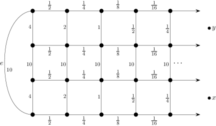
Figure 10: An example showing that Conjecture 6.1 is false if $|$G$|_{\ell}$ is not compact.

MacLane’s well-known planarity criterion chartacterises planar graphs in algebraic terms (see also [13, Theorem 4.5.1]):

Theorem 6.2 ([35]).

A finite graph is planar if and only if its cycle space $\mathcal{C}(G)$ has a simple generating set.

A generating set of $\mathcal{C}(G)$ is called simple if no edge appears in more than two of its elements.

Bruhn and Stein generalised Theorem 6.2 to locally finite graphs [7]. Our next conjecture is an attempt to characterise all planar continua in algebraic terms in a way similar to Theorem 6.2. In order to state it, call a set $S$ of circlexes in a metric space $X$ simple if for every 1-simplex $\sigma$ in $X$ there are at most 2 elements of $S$ that have a sub-simplex homotopic to $\sigma$.

Conjecture 6.2.

Let $X$ be a compact, 1–dimensional, locally connected, metrizable space that has no cut point. Then $X$ is embeddable in $S^{2}$ if and only if there is a simple set $S$ of circlexes in $X$ and a metric $d$ inducing the topology of $X$ so that the set $U:=\{\overline{\chi}\in H_{\ell}(X)\mid\chi\in S\}$ spans $H_{\ell}$.

To see the necessity of assuming local connectedness in this conjecture, consider the space obtained from some non-planar graph after replacing an interval of each edge by a topologist’s sine curve.

The requirement that $X$ have no cut point in the conjecture is also necessary. Indeed, let $G$ be the infinite 2-dimensional grid, let $I$ be the real unit interval, and let $X$ be the topological space obtained from $|G|$ and $I$ by identifying the end of $G$ with an endpoint of $I$ —which is now a cut point of $X$. It is easy to see that $X$ is not embeddable in $S^{2}$, although it satisfies all other requirements of Conjecture 6.2.

7 Line graphs

In this section we are going to prove Theorem 1.4; let us repeat it here:

Theorem.

If $G$ is a countable graph and $ETOP(G)$ has a topological Euler tour then $MTOP({L(G)})$ has a Hamilton circle.

Before proving this, let me argue that it is indeed necessary to use both topologies $ETOP$ and $MTOP$ in its statement (we can replace $ETOP$ by $ETOP^{\prime}$ though).

Firstly, if $G\$is a non-locally-finite graph then $MTOP$($G$) never has a topological Euler tour: for if $\sigma:S^{1}\to MTOP($G$)$ is such a topological Euler tour and $x$ a vertex of $G\$of infinite degree, then as $\sigma$ has to traverse all the edges incident with $x$, its domain $S^{1}$ must contain a point $z$ that is an accumulation point of an infinite set of intervals each of which is mapped to a distinct edge of $x$. This point $z$ can only be mapped to $x$ by $\sigma$, but as $x$ has open neighbourhoods in $MTOP$($G$) that contain no other vertex except $x$, $\sigma$ fails to be continuous at the point $z$, a contradiction. On the other hand, if $G\$is a countable connected graph then it follows from Lemmas 7.1 and 7.2 below that the existence of a topological Euler tour in $ETOP(G)$ is equivalent to the assertion that $G\$has no finite cut of odd cardinality. Thus the “right” topology to look for a topological Euler tour is $ETOP$.

What if we try to replace $MTOP({L(G)})$ in Theorem 1.4 by $ETOP(L(G))$? Consider the graph $G$ in Figure 11. For this graph we can easily find a topological Euler tour in $ETOP(G)$. Moreover, $ETOP(L(G))$ consists of $L(G)$ and precisely one additional point $\omega$, namely, the equivalence class containing $\{e,f,g,h\}$ and the unique edge-end of $L(G)$. Thus, if there is a Hamilton circle $H$ in $ETOP(L(G))$, then $H$ must consist of $\omega$ and a double ray containing all vertices of $L(G)$ except $e,f,g$ and $h$. But it is easy to see that such a ray does not exist in $L(G)$. One way to go around this is to consider the topology $ETOP^{\prime}(L(G))$ istead of $ETOP(L(G))$, that is, consider $\{e,f,g,h\}$ as distinct points with the same set of open neighbourhoods. In this case we would obtain a Hamilton circle in $ETOP^{\prime}(L(G))$, but the interested reader can check that no such Hamilton circle $H$ can have the property that every vertex of $L(G)$ is incident with two edges in $H$: some of the vertices $e,f,g,h$ would have to be an accumulation point in $H$ of other vertices. The Hamilton circle $H$ we are going to construct in the proof of Theorem 1.4 however, does have the property that every vertex $x$ is incident with two edges in $H$: since $x$ has open neighbourhoods in $MTOP({L(G)})$ that contain no other vertex, a continuous injective mapping $\tau:S^{1}\to MTOP({L(G)})$ can only reach $x$ along an edge and must use another edge to leave it.

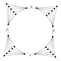
Figure 11: A case in which $ETOP(G)$ is eulerian but $ETOP(L(G))$ is not hamiltonian.

We will now prove Theorem 1.4. In order to do so we will first need to characterize the graphs $G\$for which $ETOP(G)$ has a topological Euler tour. This is achieved by the following two lemmas.

Lemma 7.1.

If $ETOP(G)$ or $ETOP^{\prime}(G)$ has a topological Euler tour then $G\$has no finite cut of odd cardinality.

Proof.

Since a topological Euler tour in $ETOP^{\prime}(G)$ easily induces a topological Euler tour in $ETOP(G)$ (by replacing each point with its equivalence class) it suffices to prove the assertion for $ETOP(G)$. Let $F$ be a finite cut of $G$, and let the set $F^{\prime}\subset ETOP(G)$ consist of a choice of one inner point from each edge in $F$. Then by the definition of $ETOP^{\prime}(G)$, $ETOP(G)\ \backslash F^{\prime}$ is the union of two disjoint open sets. It is now easy to see that any continuous image of $S^{1}$ in $ETOP(G)$ must “cross” $F$ an even number of times, proving that if $|F|$ is odd then $ETOP(G)$ cannot have a topological Euler tour. ∎

In [24, Theorem 4] it was proved that if for a locally finite graph $G\$there is a topological Euler tour $\sigma$ in $|G|$, then $\sigma$ can be chosen so that it visits every end of $G\$precisely once. Our next lemma extends this to a countable $G$. The aforementioned statement was used in the same paper to prove the locally finite version of Theorem 1.4, by starting with such a topological Euler tour $\sigma$ of $G\$and modifying it in the obvious way to obtain a Hamilton circle $H$ of $L(G)$; the extra condition on $\sigma$ was used there to make sure that $H$ visits no end of $L(G)$ more than once. Similarly, the now more elaborate condition on $\sigma$ in the following lemma will be necessary in order to make sure that the Hamilton circle we will be constructing in the proof of Theorem 1.4 will be injective at the boundary points.

Lemma 7.2.

If $G\$is a countable connected graph that has no finite cut of odd cardinality then $ETOP^{\prime}(G)$ has a topological Euler tour $\sigma$. Moreover, $\sigma$ can be chosen so that for every two distinct points $x,y\in S^{1}$ each of which is an accumulation point of preimages (under $\sigma$) of vertices of $G$, the points $\sigma(x)$ and $\sigma(y)$ can be separated in $ETOP^{\prime}(G)$ by finitely many edges (in particular, $\sigma(x)\neq\sigma(y)$).

Proof.

Clearly $G$ has a finite cycle $C$, because otherwise every edge would be a cut of cardinality 1. Fix a continuous function $\sigma_{0}:S^{1}\to C$, that maps a closed, non-trivial interval of $S^{1}$ to each vertex and edge of $C$ (here an edge contains its endvertices).

We will now inductively, in $\omega$ steps, define a topological Euler tour $\sigma$ in $ETOP^{\prime}(G)$. After each step $i$ we will have defined a finite set of edges $F_{i}$ and a continuous surjection $\sigma_{i}:S^{1}\to\overline{F_{i}}$, where $\overline{F_{i}}$ is the subspace of $ETOP^{\prime}(G)$ consisting of all edges in $F_{i}$ and their incident vertices. In addition, we will have chosen a set of vertices $S_{i}$ in $\overline{F_{i}}$, with the property that every component of $G-F_{i}$ is incident with at most one vertex in $S_{i}$. For each vertex $v\in S_{i}$, we will choose a closed interval $I_{v}=I^{i}_{v}$ of $S^{1}$ mapped to $v$ by $\sigma_{i}$. (These intervals will be used in subsequent steps to accommodate the parts of the graph not yet in the image of $\sigma_{i}$). Then, at step $i+1$, we will pick a suitable set of finite circuits in $E(G)-F_{i}$, put them into $F_{i}$ to obtain $F_{i+1}$, and modify $\sigma_{i}$ to $\sigma_{i+1}:S^{1}\to\overline{F_{i+1}}$. We might also add some vertices to $S_{i}$ to obtain $S_{i+1}$.

To begin with, let $F_{0}=E(C)$, $S_{0}=\emptyset$ and $\sigma_{0}$ as defined above. Let $e_{1},e_{2},\ldots$ be an enumeration of the edges of $G$. Then, for $i=1,2,\ldots$, perform a step of the following type. In step $i$, let for a moment $S_{i}=S_{i-1}$ and consider the components of $G-F_{i-1}$, which are finitely many since $F_{i-1}$ is finite. For every such component, say $D$, there is by the inductive hypothesis at most one vertex $v=v_{D}\in S_{i}$ incident with $D$. If there is none, then just pick any vertex $v$ incident with both $D$ and $F_{i-1}$, put it into $S_{i}$, and let $I_{v}$ be any maximal interval of $S^{1}$ mapped to $v$ by $\sigma_{i-1}$; recall that by the construction of the $\sigma_{i}$, $I_{v}$ is non-trivial.

We claim that every edge in $G-F_{i-1}$ lies in a finite cycle. Indeed, if some edge $e=wz\in E(G)\backslash F_{i-1}$ does not, then $\{e\}\cup F_{i-1}$ separates $w$ from $z$ in $G$. But then, let $\{W,Z\}$ be a bipartition of the vertices of $G$ such that $w\in W$, $z\in Z$, and there are no edges between $W$ and $Z$ in $G-(\{e\}\cup F_{i-1})$. Let $E(W,Z)$ be the set of edges in $G$ between $W$ and $Z$. Since $F_{i-1}$ is a finite edge-disjoint union of finite circuits, $|E(W,Z)\cap F_{i-1}|$ is even; thus $E(W,Z)\ni e$ is an odd cut of $G$, which contradicts our assumption.

Similarly, if $D$ is any component of $G-F_{i-1}$ and we let $j=j_{D}:=\min\{k\mid e_{k}\in E(D)\}$, then $D$ contains a finite edge-set $C_{D}$ in $D$ such that $C_{D}$ is incident with $v_{D}$, it contains the edge $e_{j}$, and $C_{D}=C_{1}\cup\ldots\cup C_{k}$ where the $C_{i}$ are pairwise disjoint finite circuits and $C_{i}$ is incident with $C_{i-1}$ for every $1<i\leq k$. Indeed, if $e_{j}$ happens to be incident with $v_{D}$ then we let $C_{D}$ consist of a single circuit containing $e_{j}$, and if not we pick a shortest $v_{D}$–$e_{j}$ path $P$, let $C_{1}$ be a finite circuit in $D$ containing the first edge of $P$, let $C_{2}$ be a finite circuit in $D-C_{1}$ containing the first edge of $P$ not in $C_{1}$, and so on; such a $C_{2}$ exists by a similar argument as in the previous paragraph. If $v$ has infinite degree then we slightly modify the choice of $C_{D}$ so that, in addition to the above requirements, $C_{D}$ contains at least $4$ edges incident with $v$. Let $F_{i}$ be the union of $F_{i-1}$ with all these edge-sets $C_{D}$, one for each component $D$ of $G-F_{i-1}$.

Then, to obtain $\sigma_{i}$ from $\sigma_{i-1}$, for each component $D$ of $G-F_{i-1}$, let $\sigma_{i}$ map $I_{v}=I^{i-1}_{v_{D}}$ continuously to $C_{D}$, in such a way that every edge in $C_{D}$ is traversed precisely once, and each time a point $x\in I_{v}$ is mapped to some vertex $w$ (incident with $C_{D}$) there is a (closed) non-trivial subinterval $J\ni x$ of $I_{v}$ such that every point of $J$ is mapped to $w$; however, make sure that each such subinterval $J$ has length at most $2^{-i}$. This defines $\sigma_{i}$. To complete step $i$, we still have to define the interval $I^{i}_{v}$ for every $v\in S_{i}$. If step $i$ did not affect $v$ yet, that is, if we did not modify the image of $I^{i-1}_{v}$ when defining $\sigma_{i}$ from $\sigma_{i-1}$ (which happens if all edges of $v$ were in $F_{i-1}$), then we let $I^{i}_{v}:=I^{i-1}_{v}$. If we did modify the image of $I^{i-1}_{v}$, then we let $I^{i}_{v}$ be one of the maximal (closed) subintervals of $I^{i-1}_{v}$ mapped by $\sigma_{i}$ to $v$; such an interval always exists and is non-trivial by the construction of $\sigma_{i}$. If, in addition, $v$ has infinite degree, then we have to be a bit more careful with our choice of an interval $I^{i}_{v}$: by the choice of the $C_{D}$ there are at least $4$ edges in some $C_{D}$ incident with $v=v_{D}$, and so there is an inner maximal subinterval $I^{\prime}$ of $I_{v}$ mapped to $v$ by $\sigma_{i}$; we let $I^{i}_{v}:=I^{\prime}$. This completes step $i$.

We claim that for every point $x\in S^{1}$ the images $\sigma_{i}(x)$ converge to a point in $ETOP^{\prime}(G)$. Indeed, since $ETOP^{\prime}(G)$ is compact, $(\sigma_{i}(x))_{i\in\mathbb{N}}$ has a subsequences converging to a point $y$ in $ETOP^{\prime}(G)$. Moreover, by the choice of the $C_{D}$, for every edge $e_{j}\in E(G)$ there is an $i$ so that $e_{j}\in F_{m}$ holds for all $m\geq i$. Thus, for every basic open set $O$ of $y$ there is an $i$ such that the component $C$ of $G-F_{i}$ in which $y$ lives is a basic open set of $y$ (up to some half edges) contained in $O$, and so $C$ contains an element $p$ of $(\sigma_{i}(x))_{i\in\mathbb{N}}$. By the definition of the $\sigma_{i}$, if $x$ is mapped to a point $p$ by $\sigma_{i+1}$, then for all steps succeeding step $i+1$ the image of $x$ will lie in the component of $G-F_{i}$ that contains $p$. This means that $C$, and thus $O$, contains all but finitely many members of $(\sigma_{i}(x))_{i\in\mathbb{N}}$, and so the whole sequence $(\sigma_{i}(x))_{i\in\mathbb{N}}$ converges to $y$.

Hence we may define a map $\sigma:S^{1}\to ETOP^{\prime}(G)$ mapping every point $x\in S^{1}$ to a limit of $(\sigma_{i}(x))_{i\in\mathbb{N}}$.

Our next aim is to prove that $\sigma$ is continuous. For this, we have to show that the preimage of any basic open set of $ETOP^{\prime}(G)$ is open. This is obvious for basic open sets of inner points of edges. For every other point $y\in\Omega^{\prime}\cup V$, the sequence of basic open sets of $y$ that arise after deleting $F_{i},i\in\mathbb{N}$ is converging, so it suffices to consider the basic open sets of that form, and it is straightforward to check that their preimages are indeed open. Thus $\sigma$ is continuous, and since by construction it traverses each edge exactly once it is a topological Euler tour.

Call two points in $\Omega^{\prime}\cup V$ equivalent if they cannot be separated by a finite edgeset. Call a point $x\in S^{1}$ a hopping point if $x$ lies in an interval of the form $I^{i}_{v}$ for every step $i$ (but perhaps for a different vertex $v$ in different steps). We now claim that

for every two distinct hopping points $$x,y\in S^{1} \sigma(x) \sigma(y) *$$, and are not equivalent. ()

Indeed, for any point $p\in ETOP^{\prime}(G)$, there is in every step $i$ at most one vertex $v$ in $S_{i}$ meeting the component $C$ of $G-F_{i}$ in which $p$ lives. Moreover, all points equivalent to $p$ also live in $C$. Thus $I_{v}$ is the only interval of $S^{1}$ in which $p$ and its equivalent points can be accommodated. Since $I_{v}$ gets subdivided after every step, there is only one point of $S^{1}$ that can be mapped by $\sigma$ to a point equivalent to $p$.

Since by construction the only points of $S^{1}$ that can be accumulation points of preimages under $\sigma$ of vertices are the hopping points, the second part of the assertion of Lemma 7.2 follows from ($*$ ‣ 7). ∎

Proof of Theorem 1.4.

Let $G\$be a countable graph such that $ETOP(G)$ has a topological Euler tour. Then $G\$has no finite cut of odd cardinality by Lemma 7.1; thus $ETOP^{\prime}(G)$ has a topological Euler tour $\sigma$ as provided by Lemma 7.2.

Let $v$ be a vertex of infinite degree. It follows easily by the choice of the circuits $C_{D}$ and the intervals $I^{i}_{v_{D}}$ in the proof of Lemma 7.2, that whenever $\sigma$ runs into $v$ along an edge then it must also leave $v$ along an edge (rather than along an arc containing a double ray); formally, this fact can be stated as follows:

For any interval $$I S^{1} \sigma(I)=\{v\} I^{\prime}\supset I S^{1} \sigma(I^{\prime})\subseteq e e v ETOP(G) I^{\prime\prime}\supset I^{\prime} S^{1} I^{\prime\prime}\backslash I \sigma(I^{\prime\prime})\subseteq e\cup e^{\prime} e^{\prime} ETOP(G) \diamondsuit$$ of with , if there is an interval of such that where is an edge (incident with ) in , then there is an interval of such that is disconnected and , where is also an edge in . ()

(We stated ($\diamondsuit$ ‣ 7) only for vertices of infinite degree because it is only interesting for such vertices; it is trivially true for vertices of finite degree).

We are now going to transform $\sigma$ into a Hamilton circle $\tau$ of $MTOP({L(G)})$. Note that if a set $F\subseteq E(G)$ converges in $ETOP(G)$ then $F\subseteq V(L(G))$ also converges in $MTOP({L(G)})$; to see this, recall that the basic open sets in $ETOP(G)$ are defined by removing finite edge-sets, while the basic open sets in $MTOP({L(G)})$ are defined by removing finite vertex sets. Thus we can define a function $\pi$ mapping any edge-end $\omega$ of $G$ to the end of $L(G)$ to which the edge-set of any ray in $\omega$ converges, and it is straightforward to check that $\pi$ is well defined. Moreover, for any vertex $v$ of infinite degree in $G\$let $\pi^{\prime}(v)$ be the accumulation point of $E(v)$ in $MTOP({L(G)})$.

We now transform $\sigma$ into a new mapping $\sigma^{\prime}$, which we will then slightly modify to obtain the required Hamilton circle in $MTOP({L(G)})$. Let $\sigma^{\prime}:S^{1}\to|L(G)|$ be the mapping defined as follows:

• $\sigma^{\prime}$ maps the preimage under $\sigma$ of each edge $e\in E(G)$ to $e\in V(L(G))$;

• for each interval $I$ of $S^{1}$ mapped by $\sigma$ to a trail $ueye^{\prime}w$ where $u,y,w$ are vertices, define $I^{\prime}$ to be the (non-trivial) subinterval of $I$ mapped by $\sigma$ to $y$, and let $\sigma^{\prime}$ map $I^{\prime}$ continuously and bijectively to the edge $ee^{\prime}\in E(L(G))$;

• if $\sigma(x)=\omega\in\Omega^{\prime}(G)$ then let $\sigma^{\prime}(x)=\pi(\omega)$.

• if $\sigma(x)=v$ where $v$ is a vertex of infinite degree in $G\$and $x$ does not lie in an interval $I$ of $S^{1}$ mapped by $\sigma$ to a trail $ueve^{\prime}w$ (which can be the case if $x$ is a hopping point), then let $\sigma^{\prime}(x)=\pi^{\prime}(v)$.

It follows by the construction of $\sigma^{\prime}$ and ($\diamondsuit$ ‣ 7) that the image of $\sigma^{\prime}$ does not contain any vertex of $G$, in other words, that $\sigma^{\prime}(S^{1})\subseteq MTOP({L(G)})$.

By construction, $\sigma^{\prime}$ maps a non-trivial interval to every vertex it traverses, which we do not want since a Hamilton circle must be injective; however, it is easy to modify $\sigma^{\prime}$ locally to obtain a mapping $\tau:S^{1}\to|L(G)|$ that maps a single point to each vertex.

It follows easily by the continuity of $\sigma$ and the definition of $\pi$ and $\pi^{\prime}$ that $\sigma^{\prime}$, and thus $\tau$, is continuous. Since $\sigma$ is a topological Euler tour of $G$, $\tau$ visits every vertex of $L(G)$ precisely once. Moreover, the second part of the assertion of Lemma 7.2 implies that $\tau$ visits no end more than once, which means that it injective. Since $S^{1}$ is compact and $|L(G)|$ Hausdorff, Lemma 2.3 implies that $\tau$ is a homeomorphism, and thus a Hamilton circle of $MTOP({L(G)})$. ∎

Having seen Theorem 1.4 and the discussion in Section 1.5, it is natural to ask if the following is true: for every graph $G$ and $\ell:E(G)\to\mathbb{R}_{>0}$, if $|$G$|_{\ell}$ has a topological Euler tour then $|L(G)|_{\ell_{L}}$ —as defined in Section 1.5— has a Hamilton circle. This is however not the case: suppose $G$ and $\ell$ are such that $|$G$|_{\ell}$ has a topological Euler tour and the boundary of $|L(G)|_{\ell_{L}}$ contains a subspace $I$ homeomorphic to the unit interval —which can easily happen, see Theorem 4.7. Then, $|L(G)|_{\ell_{L}}$ cannot have a Hamilton circle $\tau$, because the preimage of $I$ under $\tau$ must be totally disconnected and $\tau$ would then induce a homeomorphism between $I$ and a totally disconnected set.

8 Outlook

In this paper we studied several aspects of $\ell\text{-}TOP$, proving basic facts and discussing applications. I expect that the current work will lead to interesting research in the future, and I hope that other researchers will contribute.

Some open problems were suggested here, but there are also other directions in which further work could be done. The general theory developed in this paper may offer a framework for other specific compactifications of infinite graphs that, next to the Freudenthal and the hyperbolic compactification —see Section 1.1— have applications in the study of infinite graphs and groups. A further possibility would be to study Brownian motion on the space $|$G$|_{\ell}$, and seek interactions with the study of electrical networks as discussed in Section 1.2. Finally, the new homology described in Section 5 suggests interactions between the study of infinite graphs and other spaces, e.g. like in Conjecture 6.2, that may be worth following up.

References

- [1] M.A. Armstrong. Basic Topology. Springer-Verlag, 1983.
- [2] I. Benjamini and O. Schramm. Harmonic functions on planar and almost planar graphs and manifolds, via circle packings. Invent. math., 126:565–587, 1996.
- [3] I. Benjamini and O. Schramm. Lack of sphere packing of graphs via non-linear potential theory. http://arxiv.org/abs/0910.3071, 2009.
- [4] H. Bruhn. The cycle space of a -connected locally finite graph is generated by its finite and infinite peripheral circuits. J. Combin. Theory (Series B), 92:235–256, 2004.
- [5] H. Bruhn, R. Diestel, and M. Stein. Cycle-cocycle partitions and faithful cycle covers for locally finite graphs. J. Graph Theory, 50:150–161, 2005.
- [6] H. Bruhn, S. Kosuch, and M. Win Myint. Bicycles and left-right tours in locally finite graphs. Preprint 2007.
- [7] H. Bruhn and M. Stein. MacLane’s planarity criterion for locally finite graphs. J. Combin. Theory (Series B), 96:225–239, 2006.
- [8] H. Bruhn and M. Stein. On end degrees and infinite circuits in locally finite graphs. Combinatorica, 27:269–291, 2007.
- [9] R. Carlson. Boundary value problems for infinite metric graphs. In Analysis on graphs and its applications (Exner, Pavel et al, editors), volume 77 of Proceedings of Symposia in Pure Mathematics, pages 355–368. AMS, 2008.
- [10] M. Coornaert, T. Delzant, and A. Papadopoulos. Gèomètrie et thèorie des groupes. Les groupes hyperboliques de Gromov, volume 1441 of Lecture notes in Math. Springer-Verlag, 1990.
- [11] R. Diestel. Locally finite graphs with ends: a topological approach. Preprint 2009.
- [12] R. Diestel. The cycle space of an infinite graph. Comb., Probab. Comput., 14:59–79, 2005.
-
[13]
R. Diestel.
Graph Theory (3rd edition).
Springer-Verlag, 2005.
Electronic edition available at:
http://www.math.uni-hamburg.de/home/diestel/books/graph.theory. - [14] R. Diestel. End spaces and spanning trees. J. Combin. Theory (Series B), 96:846–854, 2006.
- [15] R. Diestel and D. Kühn. Graph-theoretical versus topological ends of graphs. J. Combin. Theory (Series B), 87:197–206, 2003.
- [16] R. Diestel and D. Kühn. On infinite cycles I. Combinatorica, 24:68–89, 2004.
- [17] R. Diestel and D. Kühn. On infinite cycles II. Combinatorica, 24:91–116, 2004.
- [18] R. Diestel and D. Kühn. Topological paths, cycles and spanning trees in infinite graphs. Europ. J. Combinatorics, 25:835–862, 2004.
- [19] R. Diestel and P. Sprüssel. The homology of locally finite graphs with ends. To appear in Combinatorica.
- [20] W. J. Floyd. Group completions and limit sets of Kleinian groups. Invent. math., 57:205–218, 1980.
- [21] H. Freudenthal. Über die Enden topologischer Räume und Gruppen. Math. Zeitschr., 33:692–713, 1931.
- [22] A. Georgakopoulos. Cycle decompositions in graphs and continua. In Preparation.
- [23] A. Georgakopoulos. Uniqueness of electrical currents in a network of finite total resistance. Preprint 2009.
- [24] A. Georgakopoulos. Infinite hamilton cycles in squares of locally finite graphs. Adv. Math., 220:670–705, 2009.
- [25] A. Georgakopoulos. Topological circles and Euler tours in locally finite graphs. Electronic J. Comb., 16:#R40, 2009.
- [26] A. Georgakopoulos and P. Sprüssel. Geodetic topological cycles in locally finite graphs. Electronic J. Comb., 16:#R144, 2009.
- [27] E. Ghys and P. de la Harpe. Sur les groupes hyperboliques, d’après M. Gromov, volume 83 of Progress in Math. Birkhäuser, Boston, 1990.
- [28] M. Gromov. Hyperbolic Groups. In Essays in group theory (ed. S. M. Gersten), MSRI series vol. 8, pages 75–263. Springer, New York, 1987.
- [29] D.W. Hall and G.L. Spencer. Elementary Topology. John Wiley, New York 1955.
- [30] A. Hatcher. Algebraic Topology. Cambrigde Univ. Press, 2002.
- [31] I. Kapovich and N. Benakli. Boundaries of hyperbolic groups. In Combinatorial and Geometric Group Theory (R. Gilman et al, editors), volume 296 of Contemporary Mathematics, pages 39–94. 2002.
- [32] B. Krön. End compactifications in non-locally-finite graphs. Math. Proc. Cambridge Phil. Soc., 131:427–443, 2001.
- [33] B. Krön and R. Möller. Metric ends, fibers and automorphisms of graphs. Math. Nachr., 281(1):62–74, 2008.
- [34] R. Lyons and Y. Peres. Probability on Trees and Networks. Cambridge University Press. In preparation, current version available at http://mypage.iu.edu/~rdlyons/prbtree/prbtree.html.
- [35] S. MacLane. A combinatorial condition for planar graphs. Fund. Math., 28:22–32, 1937.
- [36] D. Vogt R. Meise. Introduction to Functional Analysis. Oxford University Press, 1997.
- [37] M. Schulz. Der Zyklenraum nicht lokal-endlicher Graphen (in german). Master’s thesis, Universität Hamburg, 2005.
- [38] H. Short (editor). Notes on Hyperbolic Groups. http://www.cmi.univ-mrs.fr/~hamish/.
- [39] P. M. Soardi and W. Woess. Uniqueness of currents in infinite resistive networks. Discrete Appl. Math., 31(1):37–49, 1991.
- [40] M. Stein. Forcing highly connected subgraphs. J. Graph Theory, 54:331–349, 2007.
- [41] C. Thomassen. Resistances and currents in infinite electrical networks. J. Combin. Theory (Series B), pages 87–102, 1990.