Spin transport and bipolaron density in organic polymers

Abstract

We present a theory for spin-polarized transport through a generic organic polymer connected to ferromagnetic leads with arbitrary angle $\theta$ between their magnetization directions, taking into account the polaron and bipolaron states as effective charge and spin carriers. Within a diffusive description of polaron-bipolaron transport including polaron-bipolaron conversion, we find that the bipolaron density depends on the angle $\theta$. This is remarkable, given the fact that bipolarons are spinless quasiparticles, and opens a new way to probe spin accumulation in organic polymers.

1 Introduction

Recent years have witnessed significant advances in organic electronics, with interesting new fundamental insights and the prospect of new applications and devices functioning at room temperature [1, 2]. A particularly interesting aspect comes from the spin degree of freedom, leading to “plastic spintronics” [3]. Organic materials such as polymers may be superior to inorganic semiconductor devices because of their small spin-orbit and hyperfine couplings, in principle allowing for very long spin coherence times. Moreover, the ease of fabrication and low-temperature processing of organic materials is very attractive for possible applications. Spin transport through $\pi$-conjugated semiconducting organic polymers has consequently been studied in a number of recent experiments, and evidence for spin-polarized current injection and giant magnetoresistance in organic spin valves [4, 5, 6, 7] as well as spin-dependent optical effects [8, 9] have been reported.

Besides relevance for applications, the unconventional electronic properties of conducting polymers pose interesting fundamental questions. In undoped trans-polyacetylene, the charge and spin carriers are known to be soliton-like excitations, which are characterized by nontrivial spin-charge relations reflecting electron fractionalization [10]. This raises the possibility of unconventional spin-transport properties in undoped trans-polyacetylene. On the other hand, for basically all doped (nondegenerate) polymers, it has been established that the dominant charge and spin carriers at low energy scales well below the mean-field Peierls gap $\Delta$ correspond to polarons and bipolarons [1, 10, 11], whereas solitons can safely be ignored. As the polaron carries spin 1/2 like an ordinary electron and the bipolaron is spinless, spin current can only be carried by the polaron. Nevertheless, as we show below, the bipolaron density is affected by spin-polarized transport and can serve as a tool to detect the latter.

In this work, we discuss spin transport through doped organic polymers, where polarons and bipolarons are the relevant charge carriers. In a typical two-terminal geometry (transport along the $x$ axis), the organic polymer is contacted at $x=0$ and $x=L$ by two ferromagnetic (FM) metallic electrodes, where $L$ is the length of the polymer. The left (right) electrode is characterized by a magnetization unit vector $\hat{m}_{L}$ ($\hat{m}_{R}$), with the angle $\theta$ between them, $\hat{m}_{L}\cdot\hat{m}_{R}=\cos\theta$. We do not attempt a microscopic modelling of the interface between a FM electrode and the organic polymer, but follow the arguments of refs. [11, 12, 13, 14], where it has been established that carriers injected into the polymer tunnel predominantly into polaron states close to the contact. We therefore impose the boundary condition that no bipolaron states near the boundaries (at $x=0$ and $x=L$) are filled by the injected current. Both contacts can then be completely described by spin-dependent conductances $G^{\uparrow}$ and $G^{\downarrow}$, which take into account the spin-dependent density of states in the FM and the (disorder-averaged) matrix elements for tunneling into polaron states [15]. Moreover, for noncollinear magnetizations ($0<\theta<\pi$), one also has to include the complex-valued mixing conductance $G^{\uparrow\downarrow}$ reflecting boundary exchange processes [16, 17, 18].

Transport in the polymer itself has so far been modelled either numerically, using lattice simulations of charge transport [19, 20, 21, 22], or analytically, using simple master equations [23] or drift-diffusion models. The latter approaches have also been applied to spin transport [24, 25, 26, 27]. Here we use the network theory of ref. [15, 16] combined with a diffusive model to obtain spin-transport properties of a doped organic polymer sandwiched between two FM electrodes with noncollinear magnetization directions (arbitrary $\theta$). In the absence of bipolarons and for very high temperatures, this problem has been studied in ref. [26]. Here we present a generalization including the polaron-bipolaron conversion process, and also study the low-temperature quantum-degenerate limit.

2 Model

The energy-dependent polaron distribution function $\hat{f}_{P}(x,\epsilon)$ at location $0<x<L$ can be decomposed into a spin-independent scalar part $f_{0}(x,\epsilon)$ and a spin-polarization vector ${\boldsymbol{f}}(x,\epsilon)$,

$$\hat{f}_{P}(x,\epsilon)=f_{0}\sigma_{0}+{\boldsymbol{f}}\cdot{\boldsymbol{\sigma}},$$ (1)

with the standard Pauli matrices $\sigma_{i}$ in spin space; $\sigma_{0}$ is the unit matrix, and we assume homogeneity in the transverse direction. Note that a polaron has charge $e$ and spin $1/2$. Another important charge carrier in organic polymers is the spinless bipolaron, with charge $2e$ and the scalar distribution function $f_{BP}(x,\epsilon)$ [1, 10]. With the average density of states $\rho(\epsilon)$, we introduce normalized densities by integrating the distribution functions over energy,

$$\hat{n}_{P}(x) = \int d\epsilon\rho(\epsilon)\hat{f}_{P}(x,\epsilon)=n_{0}(x)+{\boldsymbol{n}}(x)\cdot{\boldsymbol{\sigma}},$$

$$n_{BP}(x) = \int d\epsilon\rho(\epsilon)f_{BP}(x,\epsilon).$$ (2)

These densities are defined relative to an equilibrium reference value, and reflect nonequilibrium charge and spin accumulation in the polymer. Since our model does not include the quasiparticle states outside the mean-field gap $\Delta$, but only retains the polaron and bipolaron states inside the gap, we choose $\rho(\epsilon)\simeq\Delta^{-1}\Theta(\Delta-|\epsilon|)$.

In typical organic polymers, disorder is present and implies diffusive transport for both polarons and bipolarons, with the respective diffusion constants $D_{P}$ and $D_{BP}$. The equations of motion for $\hat{n}_{P}(x,t)$ and $n_{BP}(x,t)$ are thus

$$\partial_{t}\hat{n}_{P} = D_{P}\partial_{x}^{2}\hat{n}_{P}-\tau_{sf}^{-1}\left(\hat{n}_{P}-n_{0}\sigma_{0}\right)+i[{\boldsymbol{h}}\cdot{\boldsymbol{\sigma}},\hat{n}_{P}]_{-}-S_{P}\sigma_{0},$$ (3)

$$\partial_{t}n_{BP} = D_{BP}\partial_{x}^{2}n_{BP}+S_{P},$$ (4)

where $\tau_{sf}$ is the polaron spin-relaxation time and $S_{P}$ models conversion processes between polarons and bipolarons [27],

$$S_{P}(x)=k\left(n_{0}^{2}-{\boldsymbol{n}}^{2}\right)-bn_{BP}.$$ (5)

The parameter $k$ describes the local recombination rate for two polarons of opposite spin forming a bipolaron, while $b$ comes from the reverse process, where a bipolaron decomposes into two polarons of opposite spin. The spin-precession term in (3) comes from an applied homogeneous magnetic field, where ${\boldsymbol{h}}=g\mu_{B}{\boldsymbol{B}}/\hbar$. We are interested in the steady-state case, where $\partial_{t}\hat{n}_{P}=\partial_{t}n_{BP}=0$ in (3) and (4). According to Fick’s law, the stationary spin-dependent particle current in the polymer is then encoded in the $2\times 2$ matrix (in spin space)

$$\hat{J}(x)=-D_{P}\partial_{x}\hat{n}_{P}(x)-D_{BP}\partial_{x}n_{BP}(x)\sigma_{0}.$$ (6)

Equation (3) yields a decoupled equation for the spin polarization vector,

$$D_{P}\partial_{x}^{2}{\boldsymbol{n}}(x)=\left(\begin{array}[]{ccc}\tau_{sf}^{-1}&-h_{z}&h_{y}\\ h_{z}&\tau_{sf}^{-1}&-h_{x}\\ -h_{y}&h_{x}&\tau_{sf}^{-1}\end{array}\right)\cdot{\boldsymbol{n}}(x).$$ (7)

Given the solution to (7), by taking the scalar part of (3) and combining it with (4), the bipolaron density is determined by

$$n_{BP}(x)=-\frac{D_{P}}{D_{BP}}\left({\cal O}\frac{x}{L}+{\cal P}+n_{0}(x)\right),$$ (8)

with two integration constants ${\cal O}$ and ${\cal P}$. The only nontrivial equation that needs to be solved is given by

$$D_{P}\partial_{x}^{2}n_{0}=k(n_{0}^{2}-{\boldsymbol{n}}^{2})+\frac{bD_{P}}{D_{BP}}\left(\frac{{\cal O}}{L}x+{\cal P}+n_{0}\right).$$ (9)

As discussed above, we impose the boundary condition

$$n_{BP}(0)=n_{BP}(L)=0,$$ (10)

since tunneling into the polymer involves only polaron states. With (8), this implies boundary conditions for (9),

$$n_{0}(0)=-{\cal P},\quad n_{0}(L)=-({\cal P}+{\cal O}).$$ (11)

In order to solve (7), we need six additional integration constants. We therefore have to specify boundary conditions reflecting spin and charge current continuity at the contacts to the left and right FMs. The FMs are taken as reservoirs with identical temperature $T$ and chemical potentials $\mu_{L/R}$, where the applied voltage is $eV=\mu_{L}-\mu_{R}$. As before, we introduce (normalized) densities,

$$n^{FM}_{L/R}=\int d\epsilon\rho(\epsilon)n_{F}(\epsilon-\mu_{L/R}),$$ (12)

with the Fermi function $n_{F}(\epsilon)=1/[e^{\epsilon/k_{B}T}+1]$. Boundary conditions then follow by relating the current (6) at $x=0$ ($x=L$) to the injected current at the left (right) interface [16],

$$\hat{J}(0) = -\sum_{\sigma=\uparrow,\downarrow}G^{\sigma}\hat{u}_{L}^{\sigma}(\hat{n}_{P}(0)-n_{L}^{FM}\sigma_{0})\hat{u}_{L}^{\sigma}-\left(G^{\uparrow\downarrow}\hat{u}^{\uparrow}_{L}\hat{n}_{P}(0)\hat{u}^{\downarrow}_{L}+{\rm h.c.}\right),$$ (13)

$$\hat{J}(L) = \sum_{\sigma=\uparrow,\downarrow}G^{\sigma}\hat{u}_{R}^{\sigma}(\hat{n}_{P}(L)-n_{R}^{FM}\sigma_{0})\hat{u}_{R}^{\sigma}+\left(G^{\uparrow\downarrow}\hat{u}^{\uparrow}_{R}\hat{n}_{P}(L)\hat{u}^{\downarrow}_{R}+{\rm h.c.}\right).$$ (14)

Note that (10) implies that bipolarons do not enter this boundary condition. The matrices $\hat{u}^{\sigma}_{L,R}=\frac{1}{2}(1+\sigma\hat{m}_{L,R}\cdot{\boldsymbol{\sigma}})$ project the spin direction $\sigma=\uparrow,\downarrow=+,-$ in the polymer onto the respective FM magnetization direction. For simplicity, we assumed identical spin-polarized ($G^{\uparrow},G^{\downarrow}$) and mixing ($G^{\uparrow\downarrow}$) conductances for both contacts. They must obey ${\rm Re}G^{\uparrow\downarrow}\geq(G^{\uparrow}+G^{\downarrow})/2$ [16]. The $2\times 2$ matrix equations (13) and (14) allow to determine the eight integration constants, and thereby yield the spin-polarized current through the system for arbitrary $\theta$. Moreover, this gives access to the bipolaron density from (8) after solving (9). We stress that none of the eight integration constants depends on the parameters $k$ and $b$ in (5).

From (6) and (8), we can immediately see that charge current $J_{c}=D_{P}{\cal O}/L$ is conserved,

$$\hat{J}(x)=J_{c}\sigma_{0}+{\boldsymbol{J}}_{s}(x)\cdot{\boldsymbol{\sigma}},$$ (15)

and the spin current, ${\boldsymbol{J}}_{s}(x)=-D_{P}\partial_{x}{\boldsymbol{n}}(x)$, follows from the solution of (7). Remarkably, both $J_{c}$ and ${\boldsymbol{J}}_{s}(x)$ are independent of the polaron-bipolaron transition rates $k$ and $b$ in (5), and the spin-dependent current alone cannot detect the presence of bipolarons in the polymer. Nevertheless, as we show below, the bipolaron density $n_{BP}(x)$, which is induced by the nonequilibrium spin accumulation in the polymer, is sensitive to these rates. As a useful measure, we will employ the integrated density,

$$N(\theta)=\int_{0}^{L}dx\ n_{BP}(x;\theta).$$ (16)

The $\theta$-dependence of the bipolaron density is then encoded in the dimensionless quantity

$$R(\theta)=\frac{N(0)-N(\theta)}{N(0)-N(\pi)}.$$ (17)

By definition, this quantity interpolates between $R(0)=0$ and $R(\pi)=1$ as $\theta$ is varied from the parallel to the antiparallel configuration.

3 Collinear case: a readily solvable limit

We first discuss a simple yet important limit, where a direct analytical solution can be obtained. This limit is defined by collinear magnetizations, $\hat{m}_{R}=p\hat{m}_{L}$ with $p=\pm$ (parallel or antiparallel configuration) and $\hat{m}_{L}=\hat{e}_{z}$. Moreover, we consider the length of the polymer as short compared to the spin coherence length, $L\ll\sqrt{D_{P}\tau_{sf}}$, and put ${\boldsymbol{h}}=0$ (no magnetic field). In that case, (7) has the general solution ${\boldsymbol{n}}(x)=-({\boldsymbol{F}}x/L+{\boldsymbol{G}})$, with constant vectors ${\boldsymbol{F}}$ and ${\boldsymbol{G}}$. For $\hat{m}_{L}=\hat{e}_{z}=\pm\hat{m}_{R}$, the boundary conditions (13) and (14) imply that the $x$ and $y$ components of both vectors vanish, and the spin current is conserved,

$${\boldsymbol{n}}(x)=-\hat{e}_{z}\left(\frac{{\cal F}}{L}x+{\cal G}\right),\quad{\boldsymbol{J}}_{s}=\frac{D_{P}{\cal F}}{L}\hat{e}_{z}.$$ (18)

The four remaining integration constants $({\cal O},{\cal P},{\cal F},{\cal G})$ readily follow by solving the boundary conditions (13) and (14) [16]. For the parallel ($p=+$) configuration, they are

$${\cal O}_{+} = 2({\cal P}_{+}+\bar{\mu})=\frac{G^{\uparrow}G^{\downarrow}+2(G^{\uparrow}+G^{\downarrow})G_{P}}{(G^{\uparrow}+2G_{P})(G^{\downarrow}+2G_{P})}eV,$$

$${\cal F}_{+} = -2{\cal G}_{+}=\frac{(G^{\uparrow}-G^{\downarrow})G_{P}}{(G^{\uparrow}+2G_{P})(G^{\downarrow}+2G_{P})}eV,$$ (19)

while for the antiparallel case, we find ${\cal F}_{-}=0$ and

$${\cal O}_{-} = -2({\cal P}_{-}+\bar{\mu})=\frac{G^{\uparrow}G^{\downarrow}}{G^{\uparrow}G^{\downarrow}+2G_{P}(G^{\uparrow}+G^{\downarrow})}eV,$$

$${\cal G}_{-} = -\frac{(G^{\uparrow}-G^{\downarrow})G_{P}}{G^{\uparrow}G^{\downarrow}+2G_{P}(G^{\uparrow}+G^{\downarrow})}\frac{eV}{2},$$ (20)

where $\bar{\mu}=(\mu_{L}+\mu_{R})/2$ is the mean chemical potential and $G_{P}\equiv D_{P}/L$. The charge current for the respective configuration is then $J_{c}=G_{P}{\cal O}_{\pm}$, while the spin current is ${\boldsymbol{J}}_{s}=G_{P}{\cal F}_{\pm}\hat{e}_{z}$.

The remaining task is to solve (for given $p=\pm$) the nonlinear equation (9) for $n_{0}(x)$ under the boundary condition (11), using (18), (19) and (20). Since the transition rates $k$ and $b$ are known to be small [27], we use a perturbative iteration scheme and write

$$n_{0}(x)=-\frac{{\cal O}}{L}x-{\cal P}+\tilde{n}_{0}(x).$$ (21)

For $k=b=0$, this Ansatz solves (9) under the correct boundary conditions when putting $\tilde{n}_{0}(x)=0$; note that the bipolaron density is directly proportional to $\tilde{n}_{0}(x)$, see (8). For small but finite $k,b$, we then insert (21) into (9) and linearize in $\tilde{n}_{0}$. This yields a second-order differential equation for $\tilde{n}_{0}(x)$, which needs to be solved under Dirichlet boundary conditions at $x=0$ and $x=L$. The solution gives the bipolaron density for the parallel and antiparallel configuration in closed form,

$$n^{(p=\pm)}_{BP}(x) = -\frac{k}{D_{BP}}\Biggl{(}{\cal C}_{\pm}x+({\cal P}_{\pm}^{2}-{\cal G}_{\pm}^{2})\frac{x^{2}}{2}+\frac{{\cal P}_{\pm}{\cal O}_{\pm}-{\cal F}_{\pm}{\cal G}_{\pm}}{L}\frac{x^{3}}{3}$$ (22)

$$\hskip 113.81102pt+\frac{{\cal O}_{\pm}^{2}-{\cal F}_{\pm}^{2}}{L^{2}}\frac{x^{4}}{12}\Biggr{)},$$

where the integration constant ${\cal C}_{\pm}$ follows from the condition $n_{BP}(L)=0$. The integrated bipolaron density (16) is then given by

$$N_{\pm}=\frac{kL^{3}}{12D_{BP}}\Biggl{(}{\cal P}_{\pm}^{2}-{\cal G}_{\pm}^{2}+{\cal P}_{\pm}{\cal O}_{\pm}-{\cal F}_{\pm}{\cal G}_{\pm}+\frac{3}{10}({\cal O}_{\pm}^{2}-{\cal F}_{\pm}^{2})\Biggr{)}.$$ (23)

Note that $N_{+}\neq N_{-}$ follows immediately from (19) and (20), indicating that the bipolaron density indeed is sensitive to the spin accumulation in the polymer. The bipolaron density (22) is shown in figure 1, taking parameters for sexithienyl as organic spacer [26]. One clearly observes a difference between the parallel and the antiparallel configuration. Although the current is not sensitive to the polaron-bipolaron transition rates $k$ and $b$, the bipolaron density is influenced by the nonequilibrium spin accumulation in the polymer.

• 

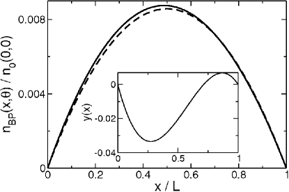
Figure 1: Bipolaron density $n_{BP}(x,\theta)$ for collinear magnetizations, i.e., $\theta=0$ (solid curve) and $\theta=\pi$ (dashed curve), as obtained from (22). We use a representative parameter set for hole transport [26]. In units where $G_{P}=D_{P}/L=1$, the parameters are $D_{BP}=2L/3,G^{\uparrow}=10^{4},G^{\downarrow}=10^{-2},k=D_{P}/10,b=D_{BP}/10$, $\Delta=3.5$, $\bar{\mu}=-2$, $T=0$, and $eV=1$. The inset shows $y(x)=[n^{(-)}_{BP}(x)-n_{BP}^{(+)}(x)]/n_{BP}^{(-)}(L/2)$ for the same curves.

4 Noncollinear magnetization

In the general case of arbitrary angle $\theta$ between $\hat{m}_{L}$ and $\hat{m}_{R}$, one can solve the problem in an analogous manner but the equations become less transparent. The main difference is that now the mixing conductance $G^{\uparrow\downarrow}$ has to be taken into account. However, as reported previously [26], we find that the results are practically independent of the precise choice for $G^{\uparrow\downarrow}$. We find a smooth crossover between the limiting values for $\theta=0$ and $\theta=\pi$, see (22), illustrated for the integrated bipolaron density (16) in figure 2.

• 

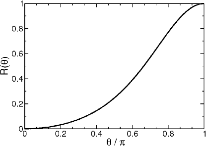
Figure 2: Spin-accumulation sensitivity $R(\theta)$, see (17), of the bipolaron density as a function of the magnetization tilt angle. Parameters are as in figure 1, additionally we set $\mbox{Re}G^{\uparrow\downarrow}=\mbox{Im}G^{\uparrow\downarrow}=5.1\times 10^{3}$.

5 Conclusions

In this work, we have discussed spin transport in doped organic polymers, employing a diffusive description of polaron and bipolaron transport. In a two-terminal setup, where the polymer is sandwiched by (generally noncollinear) ferromagnetic electrodes, the problem can be solved analytically by exploiting the smallness of the polaron-bipolaron transition rates $k$ and $b$. While the spin-dependent current through the device turns out to be independent of $k$ and $b$, the nonequilibrium bipolaron density is a sensitive probe of spin accumulation. The possibility to measure this density in optical-absorption experiments [28, 29, 30], e.g., by adapting charge-modulation techniques [31] to the two-terminal transport geometry considered here, may offer a novel way to probe spin accumulation in organic polymers. Such an optical method would be complementary to the usual magnetoresistance measurement of spin accumulation and could thus serve as another means to independently verify spin-injection efficiencies in organic polymers [32].

Our work generalizes previous studies where bipolarons were neglected [26] or only a single ferromagnet-polymer interface was considered [27]. We also treat the nonequilibrium situation due to an applied voltage self-consistently instead of postulating the existence of a uniform electric field [27]. We mention in passing that results from a recent Monte Carlo simulation [33] have elucidated the importance of bipolaronic effects for a nontraditional type of magnetoresistance that occurs in conducting polymers in the absence of magnetic contacts. Another recent theoretical study [34] on magnetoresistance in polymers with polaron and bipolaron carriers used a diffusive approach and magnetic contacts (FM-polymer-FM configuration). In contrast to our work, however, ref. [34] does not take into account conversion processes between polaron and bipolaron states, but simply assumes a constant density of bipolarons and includes this into the transport calculations. Surprisingly, a dependence of the magnetoresistance on the ratio of bipolarons and polarons is reported [34], whereas we find the spin-polarized current to be independent of the bipolaron formation rate. Our finding can be traced back to the well-established [13, 14] suppression of tunneling into bipolaron states near the interface with a FM electrode. This feature is ignored when simply asssuming a constant bipolaron density.

References

References

- [1] Campbell I H and Smith D L 2001 Solid State Physics vol 55 ed F Spaepen and H Ehrenreich (San Diego: Academic Press) p 1
- [2] Kaiser A B Adv. Mater. 13 927
- [3] Naber W J M, Faez S and van der Wiel W G 2007 J. Phys. D: Appl. Phys. 40 R205
- [4] Dediu V, Murgia M, Matacotta F C, Taliani C and Barbanera S 2002 Sol. Stat. Comm. 122 181
- [5] Xiong Z H , Wu D, Vardeny Z V and Shi J 2004 Nature 427 821
- [6] Pramanik S, Stefanita C-G, Patibandla S, Garre K, Harth N, Cahay M and Bandyopadhyay S 2007 Nat. Nanotech. 2 216
- [7] Majumdar S, Majumdar H S, Laiho R and Österbacka R 2009 New J. Phys. 11 013022
- [8] Davis A H and Bussmann K 2003 J. Appl. Phys. 93 7358
- [9] Campbell I H and Crone B K 2007 Appl. Phys. Lett. 90 242107
- [10] Heeger A J, Kivelson S, Schrieffer J R and Su W-P 1988 Rev. Mod. Phys. 60 781
- [11] Kirova N and Brazovskii S 1996 Synth. Metals 76 229
- [12] Bussac M N, Michaud D and Zuppiroli L 1998 Phys. Rev. Lett. 81 1678
- [13] Basko D M and Conwell E M 2002 Phys. Rev. B 66 094304
- [14] Xie S J, Ahn K H, Smith D L, Bishop A R and Saxena A 2003 Phys. Rev. B 67 125202
- [15] Brataas A, Nazarov Yu V and Bauer G E W 2000 Phys. Rev. Lett. 84 2481
- [16] Huertas Hernando D, Nazarov Yu V, Brataas A and Bauer G E W 2000 Phys. Rev. B 62 5700
- [17] Balents L and Egger R 2000 Phys. Rev. Lett. 85 3464
- [18] Balents L and Egger R 2001 Phys. Rev. B 64 035310
- [19] Magela e Silva G 2000 Phys. Rev. B 61 10777
- [20] Johansson A and Stafström S 2001 Phys. Rev. Lett. 86 3602
- [21] Johansson A and Stafström S 2002 Phys. Rev. B 65 045207
- [22] Ma H and Schollwöck U 2008 J. Chem. Phys. 129 244705
- [23] Freire J A and Voss G 2005 J. Chem. Phys. 122 124705
- [24] Ruden P P and Smith D L 2004 J. Appl. Phys. 95 4898
- [25] Ren J F, Fu J Y, Liu D S, Mei L M and Xie S J 2005 J. Phys.: Cond. Matt. 17 2341
- [26] Yu Z G, Berding M A and Krishnamurty S 2005 Phys. Rev. B 71 060408(R)
- [27] Zhang Y, Ren J, Hu G and Xie S 2008 Organic Electronics 9 687
- [28] Patil A O, Heeger A J and Wudl F 1988 Chem. Rev. 88 183
- [29] Salaneck W R, Friend R H and Brédas J L 1999 Phys. Rep. 319 231
- [30] Blythe T and Bloor D 2005 Electrical Properties of Polymers 2nd ed (Cambridge: Cambridge University Press)
- [31] Harrison M G, Fichou D, Garnier F and Yassar A 1998 Opt. Mater. 9 53
- [32] Vardeny Z V 2009 Nat. Mater. 8 91
- [33] Bobbert P A, Nguyen T D, van Oost F W A, Koopmans B and Wohlgenannt M 2007 Phys. Rev. Lett. 99 216801
- [34] Ren J, Zhang Y and Xie, S 2008 Organic Electronics 9 1017