On the X-ray emission from massive star clusters and their evolving superbubbles II. Detailed analytics and observational effects

Abstract

In this work, we present a comprehensive X-ray picture of the interaction between a super star cluster and the ISM. In order to do that, we compare and combine the X-ray emission from the superwind driven by the cluster with the emission from the wind-blown bubble. Detailed analytical models for the hydrodynamics and X-ray luminosity of fast polytropic superwinds are presented. The superwind X-ray luminosity models are an extension of the results obtained in Paper I. Here, the superwind polytropic character allows to parameterize a wide variety of effects, for instance, radiative cooling. Additionally, X-ray properties that are valid for all bubble models taking thermal evaporation into account are derived. The final X-ray picture is obtained by calculating analytically the expected surface brightness and weighted temperature of each component. All of our X-ray models have an explicit dependence on metallicity and admit general emissivities as functions of the hydrodynamical variables. We consider a realistic X-ray emissivity that separates the contributions from hydrogen and metals. The paper ends with a comparison of the models with observational data.

1 INTRODUCTION

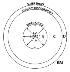
Young super star clusters (SSCs) are compact stellar aggregates resulting from intense, concentrated, violent star formation episodes. With ages between $\sim 10^{6}$–$10^{7}$ yr and masses in the range of $\sim 10^{4}$–$10^{7}$ M_⊙, they represent the current analogues of globular clusters and have been identified as the building blocks of stellar formation in many galaxies (O’connell et al. 1995; Whitmore & Schweizer 1995; Ho 1997; Whitmore et al. 1999; Melo et al. 2005 and references therein). Within its effective radius of up to a few parsecs ($\lesssim 10$-pc, Meurer et al. 1995; Melo et al. 2005), a SSC contains many thousands or tens of thousands of early-type stars (Leitherer & Heckman 1995) that dominate the injection of mass and energy ($\sim 10^{38}$–$10^{41}$ erg s^-1) to the ISM through the overall contribution of their individual stellar winds and supernovae explosions. The interactions that take place among these inner flows lead to the thermalization of their kinetic energy through strong shock waves that generate a high central over-pressure. As a result, a powerful superwind is driven out of the cluster at large speed ($\gtrsim 1000$ km s^-1). Outside of the cluster, the superwind expands almost freely until the presence of the ISM becomes important. The subsequent interaction of this supersonic and metal-rich outflow with the ambient interstellar gas generates a structure with a more complex dynamics, namely, a superbubble (Castor, McCray & Weaver 1975; Weaver et al. 1977, W77 hereafter; Koo & McKee 1992a,b; Bisnovatyi-Kogan & Silich 1995 and references therein). The configuration of a superbubble is traced by two shock fronts that are inherent to its hydrodynamical evolution: a leading (outer) shock that sweeps up, compresses and confines the ambient ISM to an external shell; and a secondary (inner) shock that propagates backwards (in the leading shock reference frame) and thermalises the kinetic energy of the free superwind. The resulting shocked gases are separated by a contact discontinuity and the thermal pressure of the hot, shocked superwind drives the outer shell. Soon, the mass of the shocked ambient gas becomes progressively larger than that of the shocked superwind. As this tendency continues, the outer shock becomes radiative, and the shocked ISM collapses into a thin, dense shell. Being more tenuous, the bubble hot interior has a larger cooling time scale and thus it remains quasi-adiabatic. This stage is called the snowplow phase. Here, in the same fashion as in Paper I, the resulting structure is split into the four zones shown in Fig. 1: region A corresponds to the star cluster volume itself, region B is the zone where the wind freely expands, region C is the superbubble that contains the shocked superwind, and region D is the outer shell where the leading shock accumulates ambient gas.

Due to the high temperatures produced by the multiple shock waves and the large amount of mass deposited by the sources, both superwinds and superbubbles are potential diffuse X-ray emitters (Chevalier 1992; Chu et al. 1995, C95 henceforth; Cantó, Raga & Rodríguez 2000; Stevens & Hartwell 2003). This represents an opportunity to study the X-ray emission associated with massive stellar clusters to better understand and constrain the ongoing hydrodynamics and its energetics. With the aid of Chandra, it has been found that several clusters in the Local Group emit an important amount of diffuse X-rays: near the centre of our Galaxy, the X-ray emissions of the Arches and Quintuplet clusters have been detected and studied by Yusef-Zadeh et al. (2002) and Law & Yusef-Zadeh (2004); that of NGC 3603 –one of the most luminous clusters in the Milky Way– has been discussed by Moffat et al. (2002); and Stevens & Hartwell (2003) have analysed R136 and NGC 346 in the Magellanic Clouds (LMC and SMC, respectively). On the other hand, Chu & Mac Low (1990) examined the Einstein archives for LMC and found seven superbubbles that were related to OB associations. Repeating later the same analysis using ROSAT data, they found four additional but dimmer superbubbles (C95). More recently, Townsley et al. (2003) have reported diffuse emission from a superbubble associated to M 17, also known as the Omega Nebula; similarly, Smith & Wang (2004) have used XMM-Newton data to study the emission from a 100-pc superbubble related to the dense OB association LH90 in 30 Dorados. In distant galaxies the X-ray emission presents two components: a system of point-like non-resolved sources, and an extended diffuse component possibly associated to a collection of superbubbles generated by individual SSCs (Summers et al. 2004; Smith, Struck & Nowak 2005).

This theoretical work has a twofold objective. The first one is to present detailed hydrodynamic and X-ray luminosity models for fast polytropic superwinds, models that can be easily modified to account for general emissivity functions (Section 2). This property allowed us to explicitly separate the X-ray contributions from hydrogen and metals and to obtain the plasma weighted temperature. These results could be of particular use when comparing with synthetic or observed spectra, since we obtained them theoretically taking into consideration bands suitable to the instruments on board Chandra and XMM-Newton. Additionally, we also present analytical formulas for the corresponding X-ray surface brightness. The second objective is to undertake the task of obtaining thoroughly all of the above for the standard analytical bubble models (Section 3). Three properties that are universal for bubbles accounting for shell evaporation are derived: an X-ray luminosity scaling factor that is independent of the particular dynamical evolution, the shape of the related surface brightness profile, and the projected X-ray temperature. We examine also the case of when the evaporation of material from the outer shell is prohibited (Section 4). Later, we assemble our models and present the complete X-ray panorama (Sections 5). Finally, we make a comparison with observational data (Section 6).

All of our X-ray models are analytical. Moreover, they are independent of the actual shape of the emissivity function because they involve hypergeometric functions. In the more general case, they can be evaluated using the code of Colavecchia & Gasaneo (2004); however, that would not be necessary here because we have constructed closed-form expansions in terms of elementary algebraic expressions. From the theoretical point of view, the freedom of selecting the emissivity function and the separation of the contributions from hydrogen and metals are advantages, since it is usual in the literature to assume a constant X-ray emissivity (C95; García-Segura & Mac Low 1995) and that the X-ray luminosity scales linearly with metallicity ($\propto Z$). The first advantage enables a more realistic modeling, and the second allows to discriminate the importance of each contribution at a given temperature and metal abundance. Our formalism also permits a straightforward calculation of other integral properties such as the luminosity of the plasma in other bands and the mass of the emitting gas (see Appendix A.2). On the hydrodynamical side, the polytropic character of the winds makes it possible to implicitly parameterize the effect of radiative cooling in a simple manner.

Figure 1: Structure of a superbubble. Each zone is defined according to its contents: region A contains the thermalised SNe and stellar wind ejecta, region B contains the free-expanding wind, region C represents the hot superbubble where the wind thermalised at the inner shock is confined, and region D is the shell that contains the swept-up ambient gas. An unperturbed ISM surrounds the structure.

Throughout the Paper, astrophysical units are used when convenient: $t_{6}$ is the time in Myr, $\dot{E}_{38}$ is the mechanical luminosity in units of $10^{38}$ erg s^-1, $R_{\rm sc,pc}$ is the star cluster radius in parsecs, $V_{8}$ is the terminal speed in units of 1000 km s^-1, $T_{\rm keV}$ is the plasma temperature at the star cluster centre in units of keV and $\Lambda_{\rm X,-23}$ is the X-ray emissivity in units of $10^{-23}$ erg s^-1cm³. A comprehensive list of symbols is given in Table 2. The reader not interested in the detailed theoretical derivations may wish to proceed directly to Sections 5 and 6.

2 POLYTROPIC SUPERWINDS

Stationary superwind models have proven valuable in reproducing the average behaviour of the star-cluster outflows obtained from full 3D hydrodynamical simulations. Although the continuous wind-source distributions assumed in the analytical models do not produce the detailed features that might result from the local interaction of stellar winds and supernovae explosions, they provide a good approximation for the radially averaged hydrodynamical profiles even for clusters with only $\sim$100 stars and become an increasingly accurate approximation as the cluster mass and stellar density also increase. Furthermore, not to far away from the cluster the agreement is better than in the inner zone because the inhomogeneities introduced by the discrete stellar population are quickly smoothed out (Cantó et al. 2000).

After a short initial transitory period, both the averaged hydrodynamical profiles and the X-ray luminosity reach almost steady values. The transitory period lasts until the cluster core is filled with shocked gas, which depends on the cluster radius and mass and energy injection rates. For instance, in their simulations, Rockefeller et al. (2005) have found this time to be $\sim 2\times 10^{4}$ yr for the Arches cluster ($R_{\rm sc,pc}\approx 0.2$ pc), whereas for the $\sim$ 5 times larger Quintuplet cluster they found it to be larger than $\sim 10^{5}$ yr. They also found small temporal variations of the X-ray luminosity: $\sim 1$ percent for the Arches cluster and around $4$–$7$ per cent for the Quintuplet cluster over a period of $\sim 50$ yr.

All of the above implies that stationary models can be used to sequentially approximate the hydrodynamical evolution of a cluster as well as the corresponding diffuse X-ray emission, given that the self-adjustment times between transitions are short and not too frequent in comparison with the cluster age and the intrinsic temporal variations of the quasi-steady states are large in comparison with the observing time. Here we present a new set of stationary wind models and obtain their associated X-ray luminosity, surface brightness and spectroscopical temperature. Certainly, the presented X-ray models do not include short-scale variations associated with interacting binaries. These are associated with the point-like X-ray sources, whose luminosity must be removed from the diffuse X-ray component (Moffat et al. 2002).

Consider the Chevalier & Clegg (1985, CC85 henceforth) fast superwind model, which assumes that the flow is steady, spherically-symmetric, adiabatic and ideal. Each star cluster can be defined by a set $\Pi_{\star}=\{R_{\rm sc},q_{\rm e},\{q_{\rm m},V_{\rm\infty A}\}\}$ containing 3 parameters: the cluster radius, $R_{\rm sc}$; the energy deposition rate per unit volume, $q_{\rm e}={\dot{E}}/{V_{\rm sc}}$; and the mass deposition rate per unit volume, $q_{\rm m}={\dot{M}}/{V_{\rm sc}}$. Alternatively, the adiabatic terminal speed $V_{\rm\infty A}=({{2q_{\rm e}}/{q_{\rm m}}})^{1/2}$ may be used. For the interior of the cluster, $r<R_{\rm sc}$ (region A), the equations of conservation of mass and momentum are

$$\rho=\frac{q_{\rm m}r}{3u}$$ (1)

and

$$\rho u\frac{{\rm{d}}u}{{\rm{d}}r}=-\frac{{\rm{d}}P}{{\rm{d}}r}-q_{\rm m}u,$$ (2)

respectively. Above, only models with finite central densities ($\rho_{\rm c}>0$) are considered, i.e. it is a requirement that $u_{\rm c}=u(0)=0$ km s^-1. For region B, the corresponding equations are

$$\rho=\frac{\dot{M}}{4\pi ur^{2}}$$ (3)

and

$$\rho u\frac{{\rm{d}}u}{{\rm{d}}r}=-\frac{{\rm{d}}P}{{\rm{d}}r}.$$ (4)

For both regions, the conservation of energy can be stated as a steady state Bernoulli-like equation

$$\epsilon=\frac{1}{2}u^{2}+\frac{\gamma}{\gamma-1}\frac{P}{\rho}=\frac{1}{2}V_{\rm\infty A}^{2},$$ (5)

where $\epsilon$ is the total energy per unit mass. Since the gas is adiabatic and perfect, $\gamma={5}/{3}$. Let’s consider now a polytropic perfect gas with equation of state

$$P=K\rho^{\frac{\eta+1}{\eta}}=nkT,$$ (6)

where $\eta$ is the polytropic index and $K>0$ is a proportionality constant. This equation replaces (5) in the polytropic case, where the entropy variations are parametrized through a constant $\eta$.

The combination of (4) and (6) yields the explicit form of the energy conservation per unit mass for region B

$$\epsilon_{\rm BP}=\frac{1}{2}u^{2}+(\eta+1)\frac{P}{\rho}=\rm constant.$$ (7)

As expected, the polytropic and the CC85 solutions have the same algebraic structure on $r\geq R_{\rm sc}$. They are isomorphic through the transformations $\gamma\rightarrow({\eta+1})/{\eta}$ and $\epsilon_{\rm BP}=({1}/{2})V_{\rm\infty P}^{2}\;\;(V_{\rm\infty A}\rightarrow V_{\rm\infty P})$. The constant $V_{\rm\infty P}$ is arbitrary and is related to the temperature at $r=R_{\rm sc}$, or, equivalently, to the speed at which the superwind leaves the star cluster surface. However, this arbitrariness vanishes when additional constraints or boundary conditions related to the parameterized effects are imposed on the model, for example, $V_{\rm\infty P}<V_{\rm\infty A}$ when just dissipative processes are involved. When more specific information about the nature of the processes is available, explicit expressions for the constraints can be given as threshold lines. For region A, the isomorphism is not exactly the case; nevertheless, as discussed below, equation (7) remains a good approximation there.

A continuous gas acceleration requires of the following condition at $r=R_{\rm sc}$

$$u_{\rm sc}=\left[\frac{(\eta+1)}{\eta}\frac{P_{\rm sc}}{\rho_{\rm sc}}\right]^{1/2}<V_{\rm\infty P}.$$ (8)

The isomorphic solutions are self-similar if written in terms of the dimensionless variables $R={r}/{R_{\rm sc}}$ and $U={u^{2}}/{V_{\rm\infty P}^{2}}$

$$R=D_{1}U^{1/2}\left[1+(6\eta+5)U\right]^{-\frac{4\eta+3}{6\eta+5}},\;\;r<R_{\rm sc},$$ (9)

$$R=D_{2}U^{-1/4}\left(1-U\right)^{-\frac{\eta}{2}},\;\;\;r\geq R_{\rm sc}.$$ (10)

Figure 2: Panel (a): comparison of the adiabatic isomorphism velocity profile for region A, equation (9), with that of the pseudo-adiabatic solution, equation (16). In general, the solutions are alike for the same set of parameters. Here, $\eta={3}/{2}$ and $V_{\rm\infty P}=V_{\rm\infty A}$. Panels (b), (c) and (d): normalised velocity, density and temperature profiles for pseudo-adiabatic polytropic solutions with $\eta={3}/{2}$ (solid lines), $\eta=1$ (dashed lines) and $\eta=2$ (dotted lines), respectively. The temperature profile is by far the most sensitive to changes of $\eta$. For superwinds with terminal speeds of the order of $V_{8}\ga 1$, $T_{\rm scA}\ga 10^{7}$ K.

Accordingly, the boundary condition (8) becomes

$$U_{\rm sc}=\frac{1}{2\eta+1}.$$ (11)

From equations (9) and (10) and condition (11), one can find that for an accelerating solution

$$D_{1}=(2\eta+1)^{1/2}\left(1+\frac{6\eta+5}{2\eta+1}\right)^{\frac{4\eta+3}{6\eta+5}}$$ (12)

and

$$D_{2}=(2\eta+1)^{-1/4}\left(1-\frac{1}{2\eta+1}\right)^{\eta/2}.$$ (13)

The actual polytropic solution for the innermost region ($r<R_{\rm sc}$) can be obtained from one of the pfaffian forms related to the conservation laws. The simplest pfaffian form is

$$\left(A\rho^{2+\frac{1}{\eta}}-r^{2}\right){\rm{d}\rho}+4\rho r\,{\rm{d}}r=0,$$ (14)

with $A=9(\eta+1)K/(q_{\rm m}^{2}\eta)$. The associated ordinary differential equation is inexact, but it has a unique integrating factor: $I_{F}=\rho^{-\frac{1}{2}}$. After multiplying by it, the next solution can be found with ease

$$r^{2}+\frac{A\eta}{3\eta+2}\rho^{\frac{2\eta+1}{\eta}}+C\rho^{1/2}=0,$$ (15)

where $C$ is an arbitrary constant. Such a solution has several branches according to the values that $C$, $K$ and $\eta$ take. By using equation (7) and the transformation $\epsilon_{\rm BP}=\frac{1}{2}V_{\rm\infty P}^{2}$ as closure relations for the the true polytropic solution given by equation (15), a simple parameterization that we call the pseudo-adiabatic solution can be obtained

$$R=D_{\rm 1P}U^{1/2}\left(1+3(2\eta+1)U\right)^{-2/3}\;\;(r<R_{\rm sc}).$$ (16)

In what follows, we shall consider the polytropic solutions (16) and (10) satisfying the boundary condition (11). Thus,

$$D_{\rm 1P}=2^{4/3}(2\eta+1)^{1/2}$$ (17)

and the values of the hydrodynamical variables at $r=R_{\rm sc}$ are

$$T_{\rm sc}=\left(\frac{\eta}{\eta+1}\right)\left(\frac{1}{2\eta+1}\right)\frac{\mu_{\rm i}}{k}V_{\rm\infty P}^{2},$$ (18)

$$\rho_{\rm sc}=(2\eta+1)^{1/2}\frac{q_{\rm m}R_{\rm sc}}{3V_{\rm\infty P}},$$ (19)

and

$$P_{\rm sc}=\left(\frac{\eta}{\eta+1}\right)\left(\frac{1}{2\eta+1}\right)^{1/2}\frac{q_{\rm m}R_{\rm sc}}{3}V_{\rm\infty P},$$ (20)

where $\mu_{\rm i}$ is the mean mass per particle for a completely ionized interstellar plasma and $k$ is the Boltzmann constant. For solar abundance $\mu_{\rm i}=14/23\mu_{\rm H}$. The central values are

$$T_{\rm c}=\frac{1}{2(\eta+1)}\frac{\mu_{\rm i}}{k}V_{\rm\infty P}^{2},$$ (21)

$$\rho_{\rm c}=D_{\rm 1P}\frac{q_{\rm m}R_{\rm sc}}{3V_{\rm\infty P}},$$ (22)

and

$$P_{\rm c}=D_{\rm 1P}\left(\frac{1}{2\eta+1}\right)\frac{q_{\rm m}R_{\rm sc}}{3}V_{\rm\infty P}.$$ (23)

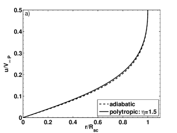
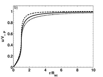
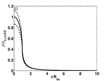
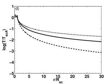
Notice that the models are valid just for $\eta>0$. For simplicity and in order to cover the polytropic states of astrophysical interest, we shall further consider that $\eta\geq{3}/{10}$ in region A. The isomorphism approaches the pseudo-adiabatic solution for large $\eta$ (the isothermal case). For intermediate values of $\eta$ they are similar [see panel (a) of Fig. 2] since they predict the same values for the hydrodynamical variables at $R_{\rm sc}$ and the same central temperature and velocity. Their densities and pressures just differ by factors of $D_{\rm 1}/D_{\rm 1P}$ at the centre and their ratios reduce towards $R_{\rm sc}$.

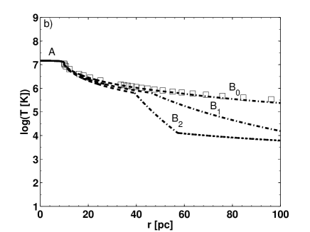
Since the effective polytropic index depends on the balance of heating and cooling among other factors, our models can parameterise these effects when complemented with acceptable boundary conditions or constraints, as we discuss next. In principle, zones with distinct entropy variations and properties can be modeled using a piecewise polytropic index, or, in the limit, a slow varying one. For the case of a continuous accelerating solution, equation (7) implies that any change in the available energy per unit mass is concomitant with a change of $\eta$ in the same direction. Nevertheless, notice that velocity discontinuities produced by shock fronts are not prohibitive. For a smooth accelerating solution with parameters $\Pi_{*}$, models with $\eta<{3}/{2}$ have higher velocity profiles and lower density profiles than the corresponding adiabatic solution ($\eta=3/2$, $V_{\infty A}=V_{\infty P}$). On the other hand, their temperature profiles have a bimodal behaviour: in region A they are higher, whereas in region B they are lower and very sensitive to the adopted value of $\eta$. Models with $\eta>{3}/{2}$ have the opposite behaviour (see Fig. 2). In the external zone, all the density profiles fall off asymptotically as $\dot{M}/4\pi V_{\rm\infty P}r^{2}$. In connection with the radiative case, Silich, Tenorio-Tagle & Rodríguez-González (2004) have shown that whilst the velocity and density profiles are barely affected by the small variations of the effective terminal speed promoted by radiative cooling, the temperature profile can be changed drastically at distances larger than a few times the star cluster radius. Given that for dissipative solutions $V_{\rm\infty P}<V_{\rm\infty A}$ and that the relative behaviour of the profiles has to scale accordingly, it follows that models with $\eta>3/2$ are appropriate for region A, whereas those with $\eta<3/2$ may be used for region B. In Fig. 3, we reproduce the numeric results of Silich et al. (2004) for radiative winds using the aforesaid method. At least 3 different $\eta$’s were required for each case presented. The profiles were constructed using the X-ray luminosity (Section 2.1) to estimate the energy radiated by the cluster core, since $\Lambda_{\rm X}\approx\Lambda_{\rm total}$ for temperatures in the order of $\sim 10^{7}$ K and $Z\approx$Z_⊙. The emissions of the external sub-zones were weighed (see Appendix A) using the total cooling function tabulated by Plewa (1995). From this, the respective changes in $V_{\rm\infty P}$ were found, and with the aid of (7), also the corresponding values of $\eta$. As a conclusion, it can be pointed out that just a change of $\eta$ (adequate for each zone) is sufficient to reproduce and explain the radiative profiles. For region A, we found that $\eta$ is always close to 3/2. However, a closed analytical estimation to find explicitly the adequate values of $\eta$ for the free wind is still lacking. In principle, just a knowledge of the star cluster parameters and the overall cooling function is sufficient to obtain it. A general discussion of the radiative case will be presented on a forthcoming paper.

Figure 3: Silich et al. (2004, fig. 4) radiative temperature profiles for clusters with $\Pi_{*}=\{R_{\rm sc,pc}=10,\dot{E}_{38}=\{500,2000,3000\},V_{8}=1\}$. They were here constructed using piecewise continuous polytropic laws. For the cluster cores (region A), $\eta\approx 3/2$ for the three mechanical luminosities. The respective free winds have different thermodynamical configurations: $B_{0}$ represents a quasi-adiabatic wind with $\dot{E}_{38}=500$, $\eta_{1}\approx 1.45$ (dashed-line) and $\eta_{2}\approx 1.15$ (dash-dotted line); likewise, $B_{1}$ is a radiative wind with $\dot{E}_{38}=2000$, $\eta_{1}\approx 1.3$ and $\eta_{2}\approx 0.42$; and $B_{2}$ is a strongly radiative wind with $\dot{E}_{38}=3000$, $\eta_{1}\approx 1.19$ and $\eta_{2}\approx 0.22$. In the later case, the velocity-radius relationship adopts $\eta=3/2$ for $T>10^{4}$ K (dotted line). The assumed metallicity is $Z=$ Z_⊙. The squares show the external temperature profile expected from the adiabatic solution, which better applies for clusters with smaller masses (mechanical luminosities).

2.1 X-ray luminosity

The cumulative X-ray luminosity of a spherically symmetric gas distribution is given by the integral

$$L_{\rm X}(r)=4\pi\int_{0}^{r}n(r^{\prime})^{2}\Lambda_{\rm X}[T(r^{\prime}),Z]r^{\prime 2}{\rm{d}}r^{\prime},$$ (24)

where $r$ is the radial coordinate from the object centre, $r^{\prime}$ the corresponding dummy integration variable, $n$ is the particle number density, and $\Lambda_{\rm X}$ is the X-ray emissivity function, which in general depends on the plasma temperature and metallicity. Here, the later is assumed homogeneous; nevertheless, tools to deal with metallicity gradients are given.

The actual dependence of the superwind X-ray emission on the star cluster parameters is determined by the functional relation of $\Lambda_{\rm X}$ with the hydrodynamical variables. This functional dependence synthesizes the physics behind the emission mechanisms. In Appendix A.1, we give an initial approximation that corresponds to a constant emissivity, whereas in Appendix A.2, we give transformation laws that are used to show how to overcome such a limitation. Those laws can also be used to incorporate the effect of metallicity gradients or non-collisional ionization equilibrium. Below, we concentrate on region A because, as is demonstrated in Appendix A.1, region B contributes less than 20 per cent to the superwind total X-ray luminosity.

In Appendix A.2, it is demonstrated that for a realistic emissivity given as piecewise continuous power laws, $\Lambda_{\rm X}=\displaystyle{\sum\Lambda_{\rm\alpha}T^{\alpha}}$, the cumulative X-ray luminosity is given by

$$L_{\rm XA}(\eta,\{\alpha\},U)=X_{A}U^{3/2}\sum_{\rm\alpha}\mathcal{F_{A}}(\eta,\alpha,U)\Lambda_{\rm\alpha}T_{\rm c}^{\alpha},$$ (25)

where

$$X_{\rm A}=\frac{D_{\rm 1P}^{5}\dot{E}^{2}}{\pi\mu_{\rm n}^{2}V_{\rm\infty P}^{6}R_{\rm sc}},$$ (26)

$$\mathcal{F_{A}}(\eta,\alpha,U)=\frac{350\left[1+\frac{\eta^{2}(8\eta+1)}{5(2\eta+1)}U^{2}\right]^{4/10}}{9\left(\frac{350}{3}+\phi_{1}U+\phi_{2}U^{2}\right)}\left(1-U\right)^{\frac{\alpha}{30}},$$ (27)

$$\phi_{1}(\eta,\alpha)=70(\alpha+28\eta+14),$$ (28)

and

$$\phi_{2}(\eta,\alpha)=[17\alpha^{2}+\alpha(501+952\eta)+9528\eta(1+\eta)+2382].$$ (29)

In these expressions $\alpha\in[-4,4]$ and $U\in[0,{1}/{(2\eta+1)}]$.

To account for a realistic emission, we assume collisional ionization equilibrium (CIE). This assumption is valid for the central region, where the ionization and recombination time-scales used to assess the collisional equilibrium (Mewe 1984, 1997) are smaller than the radiative and adiabatic expansion cooling time-scales (see Ji, Wang & Kwan 2006). Outside of the cluster, CIE does not hold for $r>2$–$3R_{\rm sc}$ ($T\lesssim 3\times 10^{6}$ K); however, the predicted X-ray emission of such region is negligible. Hence, we use the Strickland & Stevens (2000, SS00 hereafter) X-ray emissivity tables, which are based on a recent version of the Raymond & Smith (1977) code. These tables give the X-ray emissivity as a function of temperature for two energy bands appropriate for Chandra and XMM-Newton observations: a soft band that goes from 0.3–2.0 keV and a hard band from 2.0–8.0 keV. They account for continuum emission by incorporating the free-free (dominant for $T\ga$ 3 keV), the free-bound and the two photon (significant for $T\leq$ 2 keV in the energy range 1–10 keV) processes. They also account for the line emission, which dominates the spectrum at temperatures around and below 1 keV. Additionally, the contributions from hydrogen and metals were separated to allow the inclusion of arbitrary metallicities. Therefore, the total X-ray emissivity can be written as

$$\Lambda_{\rm X}(T,Z)=\Lambda_{\rm XH}(T)+Z\Lambda_{\rm XM}(T).$$ (30)

We fitted power laws and rational functions to the SS00 tables using a trust region method (see Table 3 and Table 4). As an outcome, it was found that for fast winds ( $V_{\rm\infty P}\ga 1000$ km s^-1 and $T_{\rm sc}\ga 9\times 10^{6}$ K) the hydrogen component in both bands well resembles a bremsstrahlung law, whereas the emissivity of metals has an almost constant value at high temperatures (2.6–8.6 keV) and a sharp power law behaviour at the other end (0.8–2.6 keV). Using these results (marked with $\star\star$ in Table 3) and evaluating formulas (25) and (27) at $U_{\rm sc}=1/(2\eta+1)$ we get that

$$L_{\rm XA,total}=X_{\rm A}U_{\rm sc}^{3/2}\left\{\mathcal{F_{A}}(\eta,\frac{1}{2},U_{\rm sc})\Lambda_{\rm H}T_{\rm c}^{1/2}+\right.Z\left.\left[\mathcal{F_{A}}(\eta,-\frac{5}{2},U_{\rm sc})\Lambda_{\rm M1}T_{\rm c}^{-5/2}+\mathcal{F_{A}}(\eta,0,U_{\rm sc})\Lambda_{\rm M2}T_{\rm c}^{0}\right]\right\}.$$ (31)

Figure 4: Panel (a): region A cumulative X-ray luminosity normalised by a factor of $X_{\rm A}/D_{\rm 1P}^{5}$, which contains the dependence on the cluster parameters. The values of the polytropic index are $\eta={3}/{2}$ (solid line), $\eta=1$ (dashed line) and $\eta=2$ (dotted line). Panel (b): ratio of the X-ray luminosity of metals (solid lines, region A) to that of hydrogen for different core temperatures ($T_{\rm keV}$). Here $\eta=3/2$. The dashed line is used as a reference. From bottom to top of the panel, the metallicities are 0.1,0.2,0.5,1.0,2.0 and 5.0 Z_⊙. The axes marks are logarithmically spaced for a better visualization.

Bearing in mind equations (21) and (26), and taking $\eta={3}/{2}$ we have that

$$L_{\rm XA,total}=(5.12\times 10^{33}\,\mbox{erg s${}^{-1}$})\frac{\dot{E}_{38}^{2}}{R_{\rm sc,pc}V_{8}^{5}}\left[1.00+1.32Z\left(\frac{1}{V_{8}^{6}}+\frac{1.30}{V_{8}}\right)\right],$$ (32)

or, in terms of $T_{\rm keV}$,

$$L_{\rm XA,total}=(9.31\times 10^{33}\,\mbox{erg s${}^{-1}$})\frac{\dot{E}_{38}^{2}}{R_{\rm sc,pc}T_{\rm keV}^{5/2}}\left[1.00+1.32Z\left(\frac{2.05}{T_{\rm keV}^{3}}+\frac{1.47}{T_{\rm keV}^{1/2}}\right)\right],$$ (33)

where the first and second terms between square brackets give the relative contribution from hydrogen and metals, respectively. Since a term $\propto T^{1/2}$ was factorized, the bracketed quantities show the variations of the SS00 emissivity function with respect to bremsstrahlung. The X-ray luminosity of warmer ($T_{\rm sc}<9\times 10^{6}$ K) and generally slower winds ($V_{8}<1$) can be obtained in a similar way using equations (25)–(29) together with Table 3.

In Paper I, the total X-ray luminosity of regions A and B was estimated by approximating the temperature and density by the constant values that they take at $R_{\rm sc}$ according to the CC85 adiabatic model, i.e. by setting $\rho=\rho_{\rm sc}$ and $T=T_{\rm sc}$ with $\eta=3/2$. Consequently, it was found that $L_{\rm XAB,total}=4\pi\alpha_{\rho}^{2}\Lambda_{X}(T_{\rm sc},Z)\rho_{\rm sc}^{2}R_{\rm sc}^{3}/3\mu_{\rm n}^{2}$. Explicitly, this is

$$L_{\rm X,AB}=\left(1.27\times 10^{34}\mbox{erg s${}^{-1}$}\right)\frac{\Lambda_{\rm X,-23}(T_{\rm sc},Z)\dot{E}_{38}^{2}}{R_{\rm sc,pc}V_{8}^{6}}=\left(1.08\times 10^{34}\mbox{erg s${}^{-1}$}\right)\frac{\Lambda_{\rm X,-23}(T_{\rm sc},Z)\dot{E}_{38}^{2}}{R_{\rm sc,pc}T_{\rm keV}^{3}}.$$ (34)

In the above formula, the effects of the actual thermodynamical structure of zones A and B and the realistic X-ray emissivity (SS00) were incorporated through the fiducial coefficient $\alpha_{\rho}\approx 2$, which smoothed the differences between the analytical and the numerical calculations that were carried out for winds with $V_{8}\approx 1$. Because such calculations also showed that the contribution of region B was always less than one-quarter of that of region A, the former was also incorporated into (34) through $\alpha_{\rho}$. These results agree fairly well with equations (63) and (69) which just assume a constant X-ray emissivity. In contrast, equations (32) and (33) explicitly show their physical dependence on the thermodynamical structure and the SS00 X-ray emissivity function through the numerical coefficients obtained, the separation of the contributions of hydrogen and metals, and their functional dependence on the terminal speed and temperature, respectively. Another advantage of these formulae over that of Paper I is that they can be used for very fast winds with $V_{\rm\infty P}\sim$ 2500–4500 km s^-1.

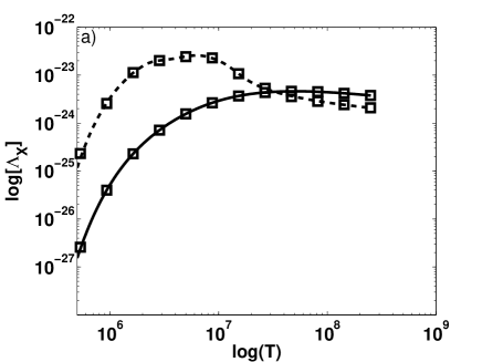
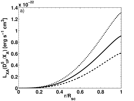
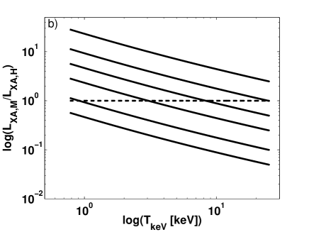
Additionally, in the current formalism, equations (25) and (16) allow to calculate the cumulative X-ray luminosity profile of region A for different polytropic indexes. If it were needed, the luminosity of region B could be calculated using our transformation laws. The cumulative X-ray luminosity profile of the cluster core for different values of $\eta$ is presented in panel (a) of Fig. 4. In the same figure, panel (b) shows that for $T_{\rm keV}\geq$ 3 keV the contribution from hydrogen is comparable (within a factor of $\sim 2$) to that from the metals when $Z\sim$ Z_⊙, whereas for lower metallicities hydrogen can dominate in the same temperature range. On the other hand, metals dominate the cluster core emission at lower temperatures when $Z\sim 0.5$–1 Z_⊙ or higher. In general, hydrogen always dominates for $Z<0.2\,$Z_⊙ and metals for $Z>2\,$ Z_⊙. We remark that metallicity gradients or a different X-ray emissivity can be handled using the aforementioned transformation laws and the adequate polytropic index. For instance, when the CIE assumption does not hold one can use non-equilibrium emissivity functions like the one presented by Gnat & Sternberg (2007), whom for solar metallicity found that $\Lambda_{\rm,noneq}\propto 5.6\times 10^{-20}T^{-0.46}$ erg s^-1 cm³. When CIE does not hold inside of the cluster, formula (25) can handle this new emissivity function with ease. By separating components and because of their ability to handle arbitrary emissivities, our formulas round out the X-ray luminosity model for the gas contained within the star cluster.

2.2 Surface brightness

To calculate the surface brightness and other projected quantities we use the Abel transform (see, e.g. Yoshikawa & Suto 1999)

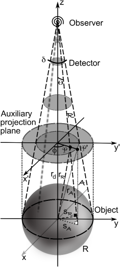
$$Q(s)=2\int_{s}^{\infty}q(r)\frac{r}{\sqrt{r^{2}-s^{2}}}{\rm{d}}r,$$ (35)

where $r$ has the same meaning as before, $s=r_{\rm d}\theta$ is the projected radius, $r_{\rm d}$ is the angular diameter distance to the object and $\theta$ the projected subtended angle. The factor of 2 takes advantage of the spherical symmetry (see Fig. 5). Since we are dealing with finitely localized gas distributions, the traditional upper limit ($\infty$) is replaced by the size of the region of interest. This size is determined by the gas temperature. We consider an X-ray cut-off temperature of $T_{\rm cut}=5\times 10^{5}$ K for all regions. The corresponding radius is $R_{\rm cut}$.

Figure 5: Abel transform of a spherically symmetric function with compact support on a ball of radius $R$ and projected angular diameter $\delta$. For $r_{\rm d}\gg R$ the Radon Transform lines (dashed), approach the Abel Transform lines (dotted) since $s_{\mathcal{R}}=r_{\rm d}\sin(\theta)\approx r_{\rm d}\theta$ and $s_{\mathcal{A}}=r_{\rm d}\tan(\theta)\approx r_{\rm d}\theta$. The right angles that the projected radii and the respective projection lines subtend are indicated with black and white squares. The spherical symmetry of the function warrants that the integral yields the same value along both lines of sight. The difference is that in the astrophysical case the distribution is projected along the $\mathcal{R}$ lines, i.e. the values at points $\wp^{\prime}$ are mapped to points $\wp$. Compare the difference in the auxiliary projection plane.

.

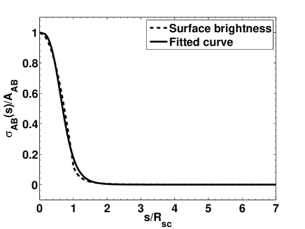
The surface brightness can be obtained by setting $q=n^{2}\Lambda_{\rm X}$ in (35). For the superwind, it is given in terms of elliptical integrals in non-canonical form, the reduction of which requires the awkward calculation of the roots of several quartics for each $s$. None the less, the whole superwind (region A+B) surface brightness can be fitted by a function of the form

$$\sigma_{\rm AB}(s)=A_{\rm AB}\left[1+\left(\frac{s}{R_{\rm sc}}\right)^{\alpha_{1}}\right]^{\alpha_{2}}.$$ (36)

For $\eta={3}/{2}$ we have that $\alpha_{1}\approx 3$ and $\alpha_{2}\approx-5/2$. The associated central brightness can be found in terms of hypergeometric functions. For fast winds, $V_{8}\gtrsim 1$, it is given by

$$A_{\rm AB}\approx 1.28\frac{\Lambda_{\rm X}(T_{\rm sc},Z)\dot{E}^{2}}{\mu_{\rm n}^{2}R_{\rm sc}^{3}V_{\infty}^{6}}=(1.9\times 10^{34}\,\mbox{erg s${}^{-1}$ pc${}^{-2}$})\frac{\Lambda_{\rm X,-23}(T_{\rm sc},Z)\dot{E}_{38}^{2}}{R_{\rm sc,pc}^{3}T_{\rm keV}^{3}}.$$ (37)

From this formula and Fig. 6, it becomes clear that even in the adiabatic case ($\eta=3/2$) the superwind X-ray surface brightness drops extremely fast ($\propto s^{-{15}/{2}}$) for $s\gg R_{\rm sc}$. Thus, although in principle clusters in the quasi-adiabatic regime per se can generate very extended X-ray emitting haloes, see equation (64), their surface brightnesses far away from the cores could be too weak to be detectable, specially when the integration times are short (see Lang et al. 2005).

Figure 6: Normalised X-ray surface brightness of a superwind ($\eta={3}/{2}$). Soft line: actual surface brightness, dashed line: fitted profile. Note that although the outer layers of the core contribute relatively more to the central X-ray luminosity (Fig. 5), no limb-brightening is produced there. The overall superwind surface brightness sharply drops in the external zone.

2.3 Weighted temperatures

Several definitions of the projected X-ray temperature exist, that is, of the temperature $T_{\rm X}$ by which the spectrum of an often multi-temperature plasma is fitted as if it would have just one component. The most frequently used ones are of the form (see e.g. Navarro, Frenk & White 1995)

$$T_{\rm X}=\frac{\int n^{2}\Lambda T\rm{d}V}{\int n^{2}\Lambda\rm{d}V},$$ (38)

where $\Lambda$ is a weighting function that may be the X-ray emissivity function (see Mazzotta et al. 2004 and references therein). The emission-measure weighting scheme uses $\Lambda=1$, whereas the so called (bolometric) emission weighting scheme assumes that $\Lambda=\Lambda(T)\propto T^{{1}/{2}}$, i.e. it assumes just free-free emission, notwithstanding the fact that this later mechanism dominates just for $T>$ 3 keV. Mazzotta et al. (2004) have shown that theoretically, none of these definitions is an accurate approximation of the spectroscopic temperature of multi-temperature plasmas. However, they have argued that since noise, instruments response, and instrumental and cosmic backgrounds among other factors affect and distort the observed spectrum, sometimes it is possible to fit a single-temperature plasma model to the data. In their work, they simulated the expected spectra of galaxy clusters ($Z=$Z_⊙) taking into account the sensitivity of the Chandra and XMM-Newton instruments in the soft band. They found that for $T\geq$ 3 keV the synthetic spectra (with temperature $T_{\rm spec}$) could be reproduced –at a level better than 5 per cent– by weighting with a function of the form $\Lambda=\Lambda(T)\propto T^{-{3}/{4}}$. Such a function yields a spectroscopic-like temperature $T_{\rm SL}$ that can be used as an estimator of the actual temperatures of the isothermal models that might be fitted to real spectral data.

None of the above schemes take into consideration arbitrary metal abundances. Vikhlinin (2006) sought to extend the previous result for $T\ga$ 0.5 keV and arbitrary metallicities. Although his algorithm yields a significant accuracy gain when lower temperatures are involved, it does not provide analytical estimations because his weighting function has to be constructed ad hoc (it depends on the measurement device characteristics and individual observational conditions). We present here a theoretical weighting scheme based on the SS00 tables. Since we do not consider observational artefacts, our spectroscopical temperature $T_{\rm X}$ corresponds to the ideal projected X-ray temperature of the models. Nevertheless, our scheme can incorporate artefacts easily, provided that the overall weighting function could be parameterized in the same way as the one found by Mazzotta el al. (2004), i.e. as a power law (or series) in $T$.

For bubbles and superbubbles we give preference to the projected temperature map as a diagnostic tool

$$T_{\rm X}(s)=\frac{\int n^{2}\Lambda T(r^{2}-s^{2})^{-1/2}r{\rm{d}}r}{\int n^{2}\Lambda(r^{2}-s^{2})^{-1/2}r{\rm{d}}r}.$$ (39)

For superwinds, the emission-measure and the Chandra and XMM-Newton spectroscopic-like temperatures (whether the later applies or not depends on $\eta$; for $\eta\approx\frac{3}{2}$, it is a valid measure when $V_{8}\ga 1.65$) can be obtained from equations (25) and (27)

$$T_{\rm X1}(\eta,{\alpha},U_{\rm sc})=\frac{L_{\rm XA}(\eta,\alpha+1,U_{\rm sc})}{L_{\rm XA}(\eta,\alpha,U_{\rm sc})}=\frac{\mathcal{F_{A}}(\eta,\alpha+1,U_{\rm sc})}{\mathcal{F_{A}}(\eta,\alpha,U_{\rm sc})}T_{\rm c},$$ (40)

where $\alpha=0$ for the first estimator and $\alpha=-3/4$ for the second one. Finally, our X-ray emission weighted temperature is

$$T_{\rm X2}(\eta,{\alpha},U_{\rm sc},Z)=\frac{L_{\rm XA}(\eta,\{\alpha+1\},U_{\rm sc})}{L_{\rm XA}(\eta,\{\alpha\},U_{\rm sc})},$$ (41)

which depends implicitly on metallicity. For superwinds with $V_{8}\gtrsim 1$, $\eta\ga{3}/{2}$ and $Z=$Z_⊙, all the above estimators yield that $T_{\rm X}\approx 0.95\,T_{\rm c}$ and that $T_{\rm X}$ gets closer to $T_{\rm c}$ as $\eta$ increases. There is just a slight difference at the other end: for $\eta\approx 0.3$ we obtained that $T_{\rm X}\approx 0.85\,T_{\rm c}$. This implies that the cluster central temperature is adequate for representing the spectroscopical one. For superwinds, ${T_{\rm sc}}/{T_{\rm c}}\in[{3}/{8},1)$, so in many cases, the temperature difference between the centre and the edge might not be significative. However, for superbubbles –as we shall see– such a difference does matter.

3 Bubbles with shell evaporation

On the theoretical side, X-ray models for superbubbles with evaporation from the cold, dense and thin outer shell (W77, region C in Fig. 1) have an interesting analytical behaviour. During the sweep-up phase, thermal conduction fluxes across the contact discontinuity promote the injection of radiatively cooled material into the cavity that contains the hotter (shock-thermalised) but much more tenuous superwind. As a result, the gas distribution has very steep density and temperature gradients and to account for the actual shape of the emissivity function becomes crucial. On the other hand, in some cases the observations pose another challenge, for after comparing with the C95 standard X-ray luminosity model, discrepancies of up to two orders of magnitude have been found (Chu, Gruendl & Guerrero 2003; Dunne et al. 2003).

Most analytical models for spherical bubbles on the sweep-up phase (Castor et al. 1975; W77; Hanami & Sakashita 1987; Koo & McKee 1992a,b; García-Segura & Mac Low 1995) share the following similarities:

1. In all models, the compact outer shell is driven by the thermal pressure of region C. There, the shocked wind is isobaric (except in a small zone near the secondary shock) and its pressure equals that of the shocked ISM. Therefore, the pressure of the hot bubble is only a function of time.

2. Similarly, it is demonstrated that the bubbles have a pseudo-adiabatic interior because the characteristic cooling time of the shocked superwind is larger than the bubble dynamical time scale (see, e.g., Mac Low & McCray 1988 and Koo & McKee 1992a,b). The prospective evaporation of cold gas from the external shell does not modify this behaviour significantly, even after the evaporated mass dominates the region.

3. Under this common premises, but considering different additional physics, the authors determined the bubble geometrical evolution and its energy budget, finding explicit expressions for the principal and secondary shock positions, the pressure, and the total energy: $R_{\rm p}(t)$, $R_{\rm s}(t)$, $P_{\rm C}(t)$ and $E_{\rm C}(t)$, respectively.

4. With exception of the Koo & McKee model, which just considers the intrinsic self-similar evolution of region C, the rest of the models assume that the thermodynamical structure is determined by the thermal evaporation of cold material from the external shell. The later process is governed by the classical thermal conduction theory (Cowie & McKee, 1977). The predicted temperature profile is of the form

   $$T_{\rm C}(r)=T_{\rm Cc}\left(1-\frac{r}{R_{\rm p}}\right)^{2/5}.$$ (42)

5. The density profile is derived from the isobaric condition stated in (i)

$$n_{\rm C}(r)=n_{\rm Cc}\left(1-\frac{r}{R_{\rm p}}\right)^{-2/5},$$ (43)

where $T_{\rm Cc}$ and $n_{\rm Cc}$ are the extrapolated central temperature and density. Note that the above profiles are spatially self-similar.

The points above imply that the dynamical evolution (linked to the motion energetics) and the thermodynamical structure are totally independent, regardless of the choice of the bubble model. Each model assumes different physical conditions that lead to different evolutions: W77 considered constant energy injection rates and ISM densities. They showed that if radiative cooling (when the bubble interior departs from a quasi-adiabatic state) and distinct ambient pressures are incorporated into their model, the bubble size can change but the self-similarity of the thermodynamical profiles is not affected. Hanami & Sakashita (1987) and García Segura & Mac Low (1995) assumed different ambient stratifications: they considered ISM densities that fall off as $\rho_{\rm 0}\propto r^{-\omega}$ and $\rho_{0}\propto r^{-2}$, respectively. The later authors also incorporated variable mechanical luminosities. Again, the geometrical expansion is different, but the shapes of the density and temperature profiles are not disturbed.

The coupling of the physics resulting from (iii) and (iv) is done through $T_{\rm Cc}$ and $n_{\rm Cc}$ which inherit the time dependence of the geometrical model, i.e. they depend on the derived $R_{\rm p}(t)$, $R_{\rm s}(t)$, $P_{\rm C}(t)$ and $E_{\rm C}(t)$. They also enclose the efficiency of the evaporative process given by the numerical value of the thermal conduction coefficient (Spitzer 1956). It can be shown that as long as conditions (iv) and (v) are satisfied, the X-ray emission and other integral properties like the evaporated mass (which dominates in this zone) are independent from the geometrical (dynamical) model. These considerations are taken into account in the X-ray models here presented, where they are used to derive properties that are valid for all evaporation dominated models. Such properties can be helpful to constraint the related physics and serve as auxiliary tools at the time of analysing the observations.

For simplicity and in order to explore the parameter space of a specific model, we shall consider that of W77, unless otherwise stated. It that model, the leading and reverse shock positions and the central temperature and density are given by

$$R_{\rm p}=(67\,\mbox{pc})\dot{E}_{38}^{1/5}n_{0}^{-1/5}t_{6}^{3/5},$$ (44)

$$R_{\rm s}=(26\,\mbox{pc})\left(\frac{\dot{E}_{38}^{3}}{n_{0}^{3}V_{8}^{5}}\right)^{1/10}t_{6}^{2/5},$$ (45)

$$T_{\rm Cc}=(5.25\times 10^{6}\,\mbox{K})\dot{E}_{38}^{8/35}n_{0}^{2/35}t_{6}^{-6/35},$$ (46)

and

$$n_{\rm Cc}=(1.63\times 10^{-2}\,\mbox{cm}^{-3})\dot{E}_{38}^{6/35}n_{0}^{19/35}t_{6}^{-22/35},$$ (47)

where $n_{0}$ is the particle number density of the ISM. For normal OB associations, McCray & Kafatos (1987) have pointed out that initially (at ages up to $5\times 10^{6}$ yr), the injection of energy (a few times $\sim 6\times 10^{35}$ erg s^-1) is dominated by the most massive but much less numerous O type stars which blow bubbles with sizes $\sim 100$ pc. At later times and up to $5\times 10^{7}$ yr, the injection rates are sustained by the supernovae explosions of B type stars; specially, after the most massive star have died. The supernovae inject energy at a steady rate of $N_{*}\alpha\times 10^{35}$ erg s^-1 (where $\alpha$ is a constant of order unity and $N_{*}$ is the total number of stars with masses above 7 M_⊙) and drive a new outflow over the previously injected gas. For rich OB associations, the wind dominated stage can be as important as the supernovae dominated one, i.e. for associations or clusters with $E_{38}\gtrsim 1$ (Abbott, Bieging & Curchwell 1981). When these effect are enhanced, models like those of Hanami & Sakashita (1987) and García-Segura & Mac Low (1995) might be more adequate to describe the evolution of the corresponding superbubbles. Here however, we follow McCray & Kafatos (1987) and assume that the energy input rate remains constant through time in order to analyse later the case of M 17.

3.1 X-ray luminosity

In its simplest form, the total X-ray luminosity of a well-developed bubble with shell evaporation is

$$L_{\rm XC,total}=4\pi n_{\rm Cc}^{2}R_{\rm p}^{3}\overline{\Lambda}_{\rm X}(\vartheta_{\rm cut},Z_{\rm C};T_{\rm Cc}),$$ (48)

where

$$\overline{\Lambda}_{\rm X}=\frac{5}{2}\int_{\vartheta_{\rm cut}}^{1}\vartheta^{1/2}(1-\vartheta^{5/2})^{2}\Lambda_{\rm X}(\vartheta,Z_{\rm C};T_{\rm Cc}){\rm d}\vartheta,$$ (49)

$\vartheta=T_{\rm C}/T_{\rm Cc}$ is the normalised temperature and $\vartheta_{\rm cut}=T_{\rm cut}/T_{\rm Cc}$ is the normalised cut-off temperature. Generally, $\Lambda_{\rm X}$ (on the integrand) cannot be put in dimensionless form with respect to $\vartheta$ and, as a consequence, it will depend on $T_{\rm Cc}$ as a parameter. The variable $\overline{\Lambda}_{\rm X}(\vartheta_{\rm cut},Z_{\rm C};T_{\rm Cc})$ can be thought as an ”evaporatively averaged” X-ray emissivity. It is practically independent of the geometrical evolution when $R_{\rm s}/R_{\rm p}<0.4$ (see Fig. 7). This is what we call a well-developed bubble and thus the upper limit of the integral in (49) is justified. For $0.4<R_{\rm s}/R_{\rm p}\leq 0.6$ there is just a slight geometrical dependence for bubbles with $T_{\rm Cc}<3\times 10^{7}$ K. If this ratio increases so does the later effect, specially in the $\sim 10^{6}$ K temperature range. Because in all current models bubbles get well-developed at early times, we shall just discuss that case.

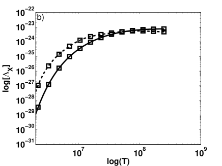
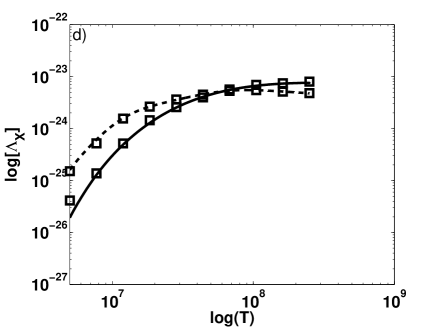
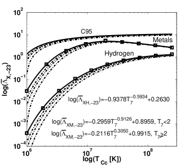
In Paper I, the bubble X-ray luminosity was estimated using the C95 model which assumes that for the Einstein satellite $\Lambda_{\rm X}(T,Z)=Z_{\rm C}\Lambda_{0}=3Z\times 10^{-23}$ erg cm³ s^-1 on the temperature range $10^{6}$–$10^{7}$ K. Therefore, one obtains that $\overline{\Lambda}_{\rm X,C95}=Z_{\rm C}\Lambda_{0}I(\vartheta_{\rm cut})$ with $I(\vartheta)=(125/33)-5\vartheta^{1/2}+(5/3)\vartheta^{3}-(5/11)\vartheta^{11/2}$. However, in some cases, the differences that arise when one considers the more realistic SS00 emissivity function can be substantial, as shown in Fig. 7. There, the average of the SS00 emissivity given by equation (30) displays separated the expected soft-band X-ray contributions from hydrogen and metals. The corresponding X-ray luminosity is

$$L_{\rm XC,total}=4\pi n_{\rm Cc}^{2}R_{\rm p}^{3}\left[\overline{\Lambda}_{\rm XH}(T_{\rm Cc})+Z_{\rm C}\overline{\Lambda}_{\rm XM}(T_{\rm Cc})\right].$$ (50)

The above formula is just corrected for the effect of the shape of $\Lambda_{\rm X}$; the variables that depend on the geometrical evolution ($R_{\rm p}$, $T_{\rm Cc}$ and $n_{\rm Cc}$) are still undetermined as functions of the problem parameters ($n_{0}$, $\dot{E}$, $V_{\rm\infty P}$) and time. Such functional relation is a consequence of the assumed bubble model. However, a great advantage of (50) is that it just depends on variables that are either directly observable or spectroscopically derivable. It is clear that the key issue is to find relationships between the central values of temperature and density and their spectroscopic estimators (Section 3.3).

On the purely theoretical side, if one also assumes the geometrical growth given by W77, an analogue to the C95 X-ray formula follows

$$L_{\rm XC,W77}=(3.25\times 10^{35}\mbox{erg s${}^{-1}$})\overline{\Lambda}_{\rm X}\dot{E}_{38}^{33/35}n_{0}^{17/35}t_{6}^{19/35},$$ (51)

where $\overline{\Lambda}_{\rm X}$ is the average of the SS00 emissivity. Since it is smaller (for all $T$) than the constant value assumed by C95, the bubbles evolve even more adiabatically and the use of the W77 model is a safe assumption. This ensures complete consistency with the emissivity function that we are using and our aim of incorporating additional physics.

Figure 7: Solid lines: evaporatively averaged soft band emissivities resulting from the C95 constant value and the SS00 tables (hydrogen: $\Lambda_{\rm XH}$, metals: $\Lambda_{\rm XM}$). Here, $T_{7}$ is $T_{\rm Cc}$ in units of $10^{7}$ K and $Z_{\rm C}=$Z_⊙. The lines for the C95 model and $\Lambda_{\rm XM}$ scale linearly with metallicity. The former was extrapolated to the temperature range $10^{6}$–$2.5\times 10^{8}$ K. The best-fitting approximations to $\Lambda_{\rm XH}$ and $\Lambda_{\rm XM}$ are shown as empty squares. Significant deviations from the C95 predicted values are observed as $T_{\rm Cc}\rightarrow 10^{6}$ K. The deviations induced by the reverse shock when $R_{\rm s}/R_{\rm p}=0.6,0.7$ and 0.8 are shown as dashed-dotted lines cascading down from the respective averaged emissivities. The axes marks are logarithmically spaced.

3.2 Surface brightness

For a single power-law X-ray emissivity, $\Lambda_{\rm X}=\Lambda_{\rm\alpha}(Z_{\rm C})T^{\alpha}$, the surface brightness was decomposed (Appendix B) into three components: a temporal component related to an intensity amplitude, $A_{\rm C}(t)$; a weighting emissivity that implicitly varies with time because of its dependence on $T_{\rm Cc}$, $\lambda_{\rm\alpha}=\Lambda_{\alpha,-23}T_{\rm Cc}^{\alpha}$ (though $\lambda_{\rm\alpha}=\lambda_{0}=3Z_{\rm C}$ is a constant for the C95 model); and a spatial profile that slowly varies with time, $S_{\rm C}(s)$ [or $\Theta(\vartheta)$ as a function of the normalised temperature]. In terms of these components $\sigma_{\rm C}(s,t)=A_{\rm C}(t)\lambda_{\rm\alpha}S_{\rm C}(s)$. Their respective model-independent expressions are given by equations (75)-(77).

For the W77 evolutionary model the amplitude factor is given by

$$A_{\rm C}(t)=(1.05\times 10^{31}\mbox{\,erg s${}^{-1}$pc${}^{-2}$ })\dot{E}_{38}^{19/35}n_{0}^{31/35}t_{6}^{-23/35}.$$ (52)

Because of the thermodynamical structure self-similarity, the shape of the spatial profile ($S_{\rm C}$) in terms of the bubble normalised projected radius ($s/R_{\rm p}$) depends solely on the the instantaneous value of the central temperature, not on the dynamical evolution. This implies that for a fixed $T_{\rm Cc}$ such a shape is the same for all bubble models accounting for shell evaporation. Note that $\lambda_{\alpha}$ is also fixed for a given $T_{\rm Cc}$ and that the prescription of a particular bubble model merely implies a scaling of the intensity amplitude. Thus, the results here presented are very general and can be applied to the overall time evolution of a single object as well as to different objects with distinct parameters at a fixed age. As we shall see, the form of the assumed X-ray emissivity will play an important role in the subsequent discussion.

Approximations for $S_{\rm C}$ as a function of temperature were implemented in equations (90) and (92) for a single power-law emissivity and the realistic SS00 emissivity, respectively. The first one allows a straightforward evaluation, while the last one, more elaborated, is necessary for a more robust discussion. In terms of $s\in[0,R_{\rm cut}]$ the former becomes

$$S_{\rm C\triangle}(s,\alpha;\xi_{\rm f},\xi_{\rm i})=\left(1-\frac{s^{2}}{R_{\rm p}^{2}}\right)^{-1/2}\left[(1-\xi)^{\frac{1+2\alpha}{5}}\mathcal{F_{C,C}}(1-s,1-\xi;\alpha)\right]_{\xi_{\rm i}=\frac{s_{\rm cut}}{R_{\rm p}}}^{\xi_{\rm f}=\max(\frac{s}{R_{\rm p}},\frac{R_{\rm s}}{R_{\rm p}})},$$ (53)

where the square-bracketed quantity written in terms of the dummy variable $\xi$ is meant to be evaluated at the indicated limits (as the result of a definite integral would), $\triangle$ indicates that we used a pseudo-triangle approximation (Appendix C), $\max({s}/{R_{\rm p}},{R_{\rm s}}/{R_{\rm p}})$ incorporates the reverse shock position and $\mathcal{F_{C,C}}(\tau,\tau_{\rm f};\alpha)$ given by equation (89) is an algebraic expression that involves the arcsin function. The central value of the spatial profile is obtained by evaluating the above equation at $s=0$. The upper limit for $\xi$ then becomes $\max(0,{R_{\rm s}}/{R_{\rm p}})={R_{\rm s}}/{R_{\rm p}}$ and we have that

$$S_{\rm C\triangle}(0,\alpha;...)=\frac{5}{1+2\alpha}\left[\left(\frac{T_{\rm Rs}}{T_{\rm Cc}}\right)^{\frac{1}{2}+\alpha}-\left(\frac{T_{\rm cut}}{T_{\rm Cc}}\right)^{\frac{1}{2}+\alpha}\right],$$ (54)

where $T_{\rm Rs}=T_{\rm Cc}(1-{R_{\rm s}}/{R_{\rm p}})^{2/5}$ is the temperature at the reverse shock position according to some specific bubble model. When $R_{\rm s}$ is ignored (which is equivalent to putting $R_{\rm s}=0$) as in the C95 X-ray luminosity model, ${T_{\rm Rs}}/{T_{\rm Cc}}$ in the previous formula becomes unity.

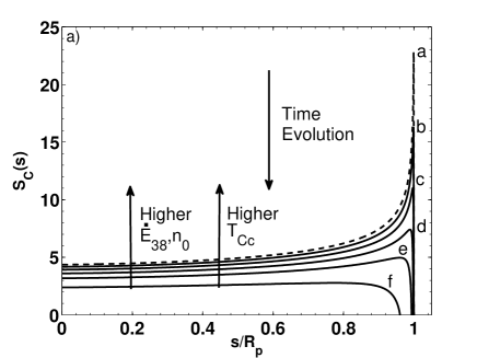
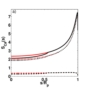
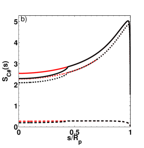
As a first step, we obtain the surface brightness corresponding to the C95 X-ray luminosity model. Theoretically, this model is equivalent to considering that the X-ray emission is proportional to the emission measure, i.e that $L_{\rm XC}=Z_{\rm C}\Lambda_{0}EM_{\rm C}$ ($\alpha=0$, $\Lambda_{\rm X}=Z_{\rm C}\Lambda_{0}$). According to this, one has that while interstellar bubbles present a practically flat profile, superbubbles driven by the most massive SSCs exhibit a noticeable limb brightening near the contact discontinuity due to their more powerful mass and energy injection rates, which translate into higher central temperatures. This is shown in panel (a) of Fig. 8. The same panel also shows the direction of the spatial profile expected time evolution for a fixed set of model parameters. As time progresses, the profile becomes flatter and weaker due to a continuous and slow decrease of the central temperature. However, the energy injection rate is not fixed as it increases by a factor of  3 after 3-Myr (Leitherer & Heckman 1995). This implies that a slight limb-brightening increment is expected for both bubbles and star clusters at this age, when the first supernovae start to explode. These results derived from our analytics and the ones presented below (Fig. 9) can also be used to reconstruct the simulated X-ray brightness profiles of Wrigge et al. (2005) for the Wolf-Rayet bubble NGC 6888. In their work, the García-Segura & Mac Low (1995) bubble model was used and the required X-ray properties were obtained by ad hoc adjusting the thermal conductivity coefficient in order to vary $T_{\rm Cc}$. We remark that the different stratification of the ISM that they considered does not produce a divergence from the analytical shape of our spatial profiles, since as it was previously stated, the thermodynamical configuration of region C is essentially the same. There are however two conspicuous differences with respect to the W77 model: in their case a) the spatial profile evolves faster ($T_{\rm Cc}\propto t^{-2/7}$ and $n_{\rm Cc}\propto t^{-12/7}$) and b) the predicted size of the bubble is not the same.

In panel (b) of Fig. 8, the C95 model is compared with one that assumes an emissivity of the form $\Lambda_{\rm X}=Z_{\rm C}\Lambda_{\rm\alpha}T^{{1}/{2}}$, i.e. a bremsstrahlung dominated emission, which is a commonly used approximation. The main difference between them is that the second one practically does not show any increment in surface brightness near the contact discontinuity. This is in better agreement with observations of the superbubbles associated to the Rosette and Omega Nebulae (Chu, Gruendl & Guerrero 2003; Townsley et al. 2001, 2003) for which no limb-brightening was detected. One then might suspect that the sharp peak predicted from a constant emissivity could be an artefact. If an emissivity that decreases towards the cut-off temperature is assumed, equation (53) reveals that the brightness is more similar to the central one. Furthermore, this also applies to the projected temperature (Section 3.3).

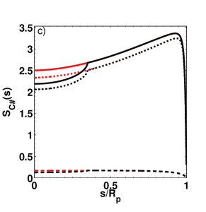
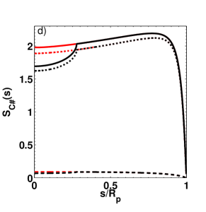
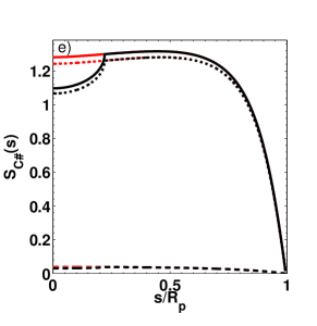
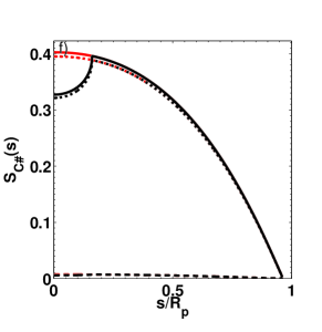
To constrain the effect of $\Lambda_{\rm X}$, we considered the SS00 X-ray emissivity function and obtained the surface brightness profile for the set of objects shown in Fig. 8. This test sample well covers the temperature range in which bubbles are observed, from a to f the central temperatures are $T_{\rm Cc}=\{3.09,1.83,1.08,0.64,0.38,0.18\}\times 10^{7}$ K. For the current analysis, it is convenient to use formula (92) –which gives the spatial profile as a function of temperature– together with Table 3. Alternatively, one can use Table 4 to numerically integrate instead of summing up. For this option, the sum symbols in (92) are replaced by $\lambda_{0}S_{\rm C\#}(s)$ with $\lambda_{0}=3$, $S_{\rm C\#}(s)=({5}/{2\Lambda_{0}})\int_{\min(\vartheta_{\rm s},\vartheta_{\rm Rs})}^{\vartheta_{\rm cut}}(\vartheta^{2}-\vartheta^{-{1}/{2}})\Lambda_{\rm X}(\vartheta,Z_{\rm C})[(1-\vartheta^{{5}/{2}})^{2}-{s^{2}}/{R_{\rm p}^{2}}]^{-1/2}\rm{d}\vartheta$ and $\Lambda_{0}=3\times 10^{-23}$ erg s^-1. The results are shown in Fig. 9. We have that in the soft band the surface brightness profile evolves a follows: it begins in a limb-brightening mode for the hottest bubbles ($T_{\rm Cc}>10^{7}$ K), later it passes through an ’unstable’ almost flat mode that occurs when the central temperature is close to $T_{\rm Cc}\approx 6.5\times 10^{6}$ K (where the X-ray emissivity has an absolute maximum for $Z\gtrsim$Z_⊙), and it ends in a limb-darkening mode (centre-brightening) for lower central temperatures ($T_{\rm Cc}\approx$ 1–2 $\times 10^{6}$ K). At early ages, $t_{6}\ll 1$, the limb-brightening can be extremely strong due to both an increase of the main peak nominal value and the visual effect produced by the relative closeness of the reverse and leading shocks. This last effect would give the central region a void appearance, if it were not for the contributions of regions A and B.

Figure 8: Panel (a): X-ray spatial profiles for the C95 X-ray model with $Z_{\rm C}=$Z_⊙. The lines scale uniformly with metallicity. From top to bottom of the panel, the central temperatures corresponding to the lines are 3.09,1.83,1.08,0.64,0.38, and 0.18, in units of $10^{7}$ K. If one assumes the W77 model, these temperatures might correspond to objects with the following parameters: lines a-d, SSCs with masses of $10^{7},10^{6},10^{5}$ and $10^{4}$ M_⊙ an age $t=3$-Myr, i.e. $\dot{E}_{38}=3000,300,30$ and $3$ (Leitherer & Heckman 1995), respectively; line e, OB association with $\dot{E}_{38}=0.3$; and line f, W77 ”typical interstellar bubble” blown by a star with $\dot{E}_{38}=0.0126$. For all cases $n_{0}=10$-cm^-3 and $V_{8}=1$. The reverse shock position is not included in the calculation. The top arrow indicates the direction of the profile time evolution for a fixed set of parameters ($E_{38},n_{0}$). The bottom arrows show how the profile varies with the energy input rate, the ISM density and the central temperature. Panel (b): spatial profile for cluster c in panel (a) when a constant emissivity ( $\alpha=0$, solid line) and a bremsstrahlung dominated one ($\alpha={1}/{2}$, dotted line) are considered. The respective pseudo-triangle approximations (Appendix C) are marked with squares. The reverse shock position was included in these models.

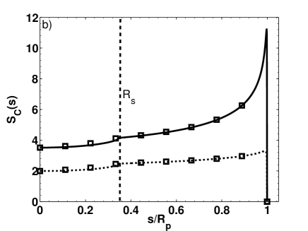
Finally, we found that the surface brightness was much smaller in the hard band. For stellar blown bubbles, the hard band emission was practically negligible. In shape, the profiles were similar to the one shown in Fig. 12.

Figure 9: Spatial profiles in the soft band for the sample shown in Fig. 8. Here, the SS00 emissivity was considered. The contributions from hydrogen (dashed lines) and metals (dotted lines) were separated. The solid lines represent the sum of both contributions. The dark lines show the profiles when $R_{\rm s}$ is included in the calculations. The red lines are obtained when the reverse shock position is neglected. Notice that by our definition, the bubbles in panels (a) and (b) are not well-developed (i.e. $R_{\rm s}/R_{\rm p}>0.4$). None the less, they have high central temperatures; thus, the position of the reverse shock does not affect their X-ray luminosity significantly (see Fig. 7).

3.3 Projected temperature

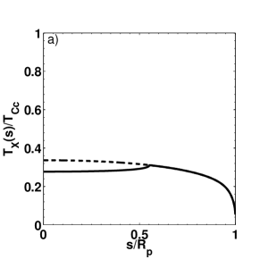
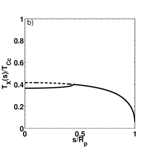
As it was indicated in Paper I, most of the superbubble X-ray emission is in the soft energy band because of the contribution of the outermost layers with temperatures in the range of $T\approx$ 5$\times 10^{5}$–$10^{6}$ K. However, the projected temperatures can be fairly larger and more similar to those near the centre of the superbubbles. In some cases, they can be of the order of $1$ keV. Superbubbles with hot interiors ($T\approx 10^{7}$ K) have already been reported by Townsley et al. (2001, 2003) and Dunne et al. (2003). In Fig. 10, we present the projected temperature curves corresponding to Fig. 9. It follows that according to the models, the spectra of shell-evaporating superbubbles could be more adequately described by a two temperature plasma model: a hot component to account for the central part and most of the bubble area, and a warm one to account for the outer layers. These theoretical temperature maps are independent from the speed of the geometrical evolution because they were derived from a ratio, see equation (39). For the hottest bubbles (i.e. when $T_{\rm Cc}\ga 10^{7}$ K), $T_{\rm X}(0)$ is a good measure of the average projected temperature inasmuch as their temperature maps are quite flat almost up to the contact discontinuity. Likewise, for ’warm’ bubbles ($T_{\rm Cc}\sim 10^{6}$ K), the projected central value is a good approximation up to half of the projected size. Because of this, in what follows we shall indistinctly refer to the average projected temperature and $T_{\rm X}(0)$ as $T_{\rm XC}$.

For the C95 model, the temperature map can be obtained from formula (53) with $\alpha=1$ normalised by itself with $\alpha=0$. The central value can be obtained in the same way from equation (54). Its low and high temperature limits are noteworthy: $T_{\rm XC}\rightarrow({1}/{3})T_{\rm Cc}$ as $T_{\rm Cc}\gg T_{\rm cut}$ and $T_{\rm XC}\rightarrow T_{\rm Cc}$ as $T_{\rm Cc}\rightarrow T_{\rm cut}$. Here, the temperature shift is an exclusive consequence of the thermodynamical structure established by evaporation. Our weighting scheme considers additionally the effect of $\Lambda_{\rm X}$ and predicts a central temperature (see Appendixes B and C)

$$T_{\rm XC}=\frac{\displaystyle{\sum_{\alpha,\vartheta_{\rm i},\vartheta_{\rm f}<\vartheta_{R_{\rm s}}}^{\vartheta_{\rm f}=\vartheta_{\rm cut}}}\left(\frac{1}{3+2\alpha}\lambda_{\alpha+1}\xi^{\frac{3}{2}+\alpha}\right)_{\xi=\vartheta_{\rm f}}^{\xi=\min(\vartheta_{\rm i},\vartheta_{\rm Rs})}}{\displaystyle{\sum_{\alpha,\vartheta_{\rm i},\vartheta_{\rm f}<\vartheta_{R_{\rm s}}}^{\vartheta_{\rm f}=\vartheta_{\rm cut}}}\left(\frac{1}{1+2\alpha}\lambda_{\alpha}\xi^{\frac{1}{2}+\alpha}\right)_{\xi=\vartheta_{\rm f}}^{\xi=\min(\vartheta_{\rm i},\vartheta_{\rm Rs})}},$$ (55)

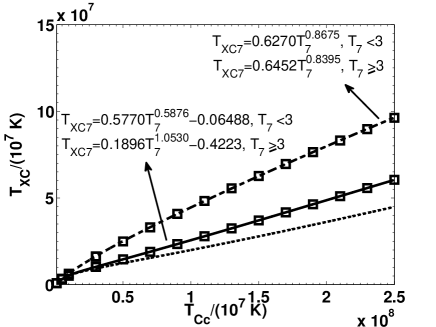
where $\vartheta_{\rm i}$ and $\vartheta_{\rm f}$ are the normalised to $T_{\rm CC}$ upper and lower temperature limits for which the power law with index $\alpha$ is valid. For a realistic emissivity the intervals and indexes are indicated in Table 3. The sum starts on the interval in which $T_{\rm Rs}$ falls. This means that the reverse shock position is embedded in the formula; none the less, given that the projected temperatures at intermediate projected radii are alike to the one obtained at the centre when $R_{s}$ is neglected (Fig. 10), it is also useful to remove its effect. This is accomplished by setting $\vartheta_{\rm Rs}=1$ (i.e. $R_{\rm s}=0$). Notice that as the coefficients $\lambda_{\alpha}$ depend on metallicity so does equation (55). The value of $T_{\rm XC}$ for different central temperatures and abundances is shown in Fig. 11. The best-fitting equations are also displayed. Note that the value of $T_{\rm XC}$ decreases as the metal abundance increases. This occurs because the emission at lower temperatures increases with the metal abundance.

Figure 10: Projected temperatures in the soft band for the bubbles shown in Fig. 8 and Fig. 9. The hottest bubbles tend to present a more uniform profile. However, the ratio of their projected temperatures to the central one is lower. In spite of this, in some cases their projected temperatures can be of the order of 1 keV.

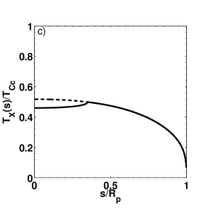
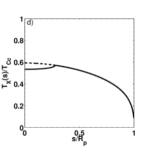
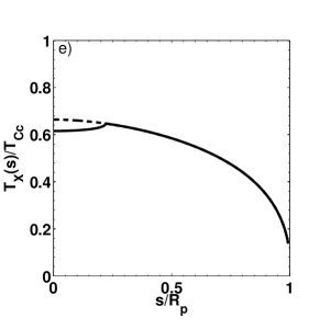
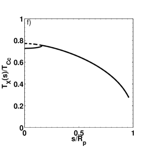
According to our analytics (i.e. no observational artefacts) $T_{\rm XC}$ just depends on the central temperature. Nevertheless, it should not be assumed to be $T_{\rm Cc}$, because it is only a fraction of the later. It should not be taken either as a temperature similar to those of the outer layers. This is particularly important for interpreting observations of hot bubbles with $T_{\rm XC}\approx 10^{7}$ K (see Section 6.2).

4 BUBBLES WITHOUT EVAPORATION

If the ISM encircling the superbubble owns an intrinsic strong magnetic field, the supposed dissemination of cold material to the hot bubble interior could be inhibited (Band & Liang 1988; Soker 1994; Dunne et al. 2003). The magnetic field prevails even after the material in question has been trapped in the cold outer shell and their components tangential to the contact discontinuity could critically hinder the evaporative process. In this case, the expression for the X-ray luminosity during the sweep-up phase is very similar to equation (10) in Paper I, but with a coefficient of 8.05 instead of 9.5 and the proper correction for the reverse and main shock positions with respect to the superbubble completely adiabatic stage.

Figure 11: Bubble projected temperature in the soft band as a function of $T_{\rm Cc}$ and metallicity. Dashed line: $Z_{\rm C}=0\,$Z_⊙, solid line: $Z_{\rm C}=$Z_⊙ and dotted line: $Z_{\rm C}=5\,$Z_⊙. The reverse shock position was neglected. Analytical expressions for the best-fitting lines (squares) to the hydrogen component and to the solar metallicity case are shown. $T_{\rm XC7}$ and $T_{7}$ are the projected and central temperatures in units of $10^{7}$ K, respectively. As expected from the shape of the emissivity function, the projected temperature decreases with increasing metallicity.

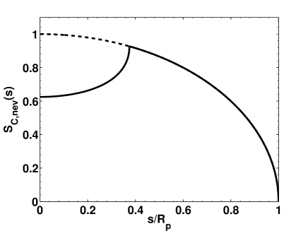
In this case, the integral that gives the surface brightness is elemental

$$\sigma_{\rm C,nev}(s)=A_{\rm C,nev}(t)\Lambda_{\rm X,-23}(\overline{T}_{\rm C},Z_{\rm C})\left[\left(1-\frac{s^{2}}{R_{\rm p}^{2}}\right)^{1/2}-\right.\left.\frac{R_{\rm s}}{R_{\rm p}}\left(1-\frac{s^{2}}{\max(s,R_{\rm s})^{2}}\right)^{1/2}\right],$$ (56)

where

$$A_{\rm C,nev}(t)=2\times 10^{-23}(1.454)^{2}\frac{(\gamma+1)^{2}\dot{E}^{2}}{4\pi^{2}\mu_{\rm n}^{2}(\gamma-1)^{2}V_{\rm\infty P}^{6}}\frac{R_{\rm p}}{R_{\rm s}^{4}}=(1.80\times 10^{30}\mbox{erg s${}^{-1}$ pc${}^{-2}$})\frac{n_{0}\dot{E}_{38}}{V_{8}^{4}}t_{6}^{-1},$$ (57)

and we have used the Koo & McKee (1992b) average post-shock density. In this case, the average temperature of the shocked gas is close to the temperature at the star cluster surface, $\overline{T}_{\rm C}\approx T_{\rm sc}$, because a fraction of the thermal energy is used to displace the outer shell of swept-up interstellar material. For very fast winds, this hot plasma is expected to emit in the hard X-ray band. The corresponding surface brightness spatial profile, $S_{\rm C,nev}$, is given by the quantity between square brackets in equation (56). It is presented in Fig. 12.

Figure 12: Surface brightness spatial profile for a superbubble generated by a cluster of $10^{5}$ M_⊙ when no evaporation occurs. Here, $t_{6}=10$ ($\dot{E}_{38}=30$), $n_{0}=10$-cm^-3 and $V_{8}=1$. The solid line traces the profile considering the reverse shock position. The dashed line indicates how the inner region would look if the reverse shock is neglected. A slight limb brightening near the reverse shock is expected together with a smooth transition to a limb darkening towards the contact discontinuity.

5 A COMPREHENSIVE X-RAY PICTURE

In Paper I, we used the total X-ray luminosity to compare the emission of superwinds and their associated superbubbles. In this paper, the corresponding X-ray models have been improved by refining the analytics and incorporating explicitly a realistic emissivity function that separates the contributions from hydrogen and metals. Here, we give a description of how to proceed in order to obtain the theoretical X-ray picture. All the parameters appearing in our formulae are expected to be derived observationally. The models can handle observational artefacts as long as they could be parameterized as power laws or series in the temperature, as in Mazzotta et al. (2004, see Sections 2.3 and 3.3).

The theoretical diffuse X-ray luminosity of the star cluster core can be obtained from equations (32) or (33). The theoretical X-ray luminosity of the free wind is $\sim 25$ per cent that of the core and its extension can be estimated from equation (64). The superwind X-ray surface brightness profile is given by equations (36) and (37) which may be helpful to extrapolate the profile of the observed diffuse emission. Estimators of the wind spectroscopic temperature ($T_{\rm X}$) are given by equations (40) and (41). All the estimators yield that for solar metallicity $T_{\rm X}$ is very close to the core central temperature, which is given by (21). The last estimator depends explicitly on $Z$. As the polytropic index was left as a free parameter, these models admit a large variety of wind configurations, as explained in Section 2.

The bubble X-ray luminosity can be obtained from (51) if the Weaver et al. (1977) model is assumed; however our approach is more general. For bubbles, once that the observational data would have been reduced and analysed, one of the first things to do for comparing with any model that considers thermal evaporation from the outer shell is to derive the theoretical central temperature, $T_{\rm Cc}$, from the one obtained for the observed spectrum. This can be done using the formulae in Fig. 11 or equation (55). With $T_{\rm Cc}$, the shape of the theoretical surface brightness profile is automatically known because it depends just on the former. For a power-law X-ray emissivity, the surface brightness profile can be obtained from (53). For a more general function, equations (92) and (93) can be used. Particularly, we have calculated the profiles that correspond to the X-ray emissivity tabulated by Strickland & Stevens (2000). These profiles are shown in Fig. 9 and can be used as a reference. Additionally, the derived value of $T_{\rm Cc}$ can be helpful to constrain the parameter space of the bubble model that one is considering, or well, to derive some parameters in order to compare them with the observations. In this regard, $T_{\rm Cc}$, the observed X-ray luminosity and the model-independent X-ray luminosity given by equation (48) can be used to compare the observationally derived electron density with the one that follows from a shell-evaporating bubble model. All of this can help to decide whether or not a specific model is adequate to describe the observations.

The X-ray luminosity of bubbles without evaporation was given in Paper I. The corresponding surface brightness is given by equations (56) and (57). The temperatures of their hot interiors are similar to the temperatures at the edges of the star clusters that generate them, equation (18).

Figure 13: Combined X-ray surface brightness of regions A, B and C. In panels (a), (b) and (c) the superbubble is blown by a 1000 km s^-1 wind generated by a cluster with a radius of 1-pc and a mass of $10^{5}$ M_⊙. The ISM density is 10-cm^-3 and $Z=Z_{\rm C}=$Z_⊙. Panel (a) shows a shell-evaporating bubble with $\dot{E}_{38}=30$ and $t_{6}=3$ ($R_{\rm p}\approx 161$-pc and $T_{\rm Cc}\approx 1.08\times 10^{7}$ K). This bubble corresponds to line c in Fig. 9, and thus, it exhibits limb-brightening near $R_{\rm p}$. In panel (c) the same $\dot{E}_{38}$ and $t_{6}$ are used but evaporation is not present; hence, the bubble has the same size than in panel (a), but it is hotter and exhibits limb-darkening towards $R_{\rm p}$. Its average temperature is $\overline{T}_{\rm C}\approx 4.42\times 10^{7}$ K. Panel (b) shows the effect of age and the smaller energy deposition rate at early times (Leitherer and Heckman 1995). The used parameters are $\dot{E}_{38}=10$ and $t_{6}=0.75$. This produces a smaller bubble with $R_{\rm p}\approx 56$-pc; however, the bubble temperature is very similar ($T_{\rm Cc}\approx 1.06\times 10^{7}$ K) to that of the bubble in panel (a). In panel (d), the surface brightness profile is almost flat because the ISM has a larger density and the star cluster is more extended and less massive: the cluster has a mass of $10^{4}$ M_⊙ and $R_{\rm sc,pc}=10$, $V_{8}=1$, $t_{6}=3$, $E_{38}=3$, $Z=Z_{\rm C}=$Z_⊙ , $n_{0}=100$-cm^-3, $R_{\rm p}=64$-pc and $T_{\rm Cc}=7.3\times 10^{6}$ K.

The main conclusion of our previous paper was that in X-rays, the superwind contribution dominates just for compact and powerful SSCs while the bubble dominates in the rest of the cases. Nevertheless, that conclusion was derived from the cumulative X-ray luminosity, which is not directly observable, but estimated from the photon counts on the detectors. What is directly observed is the surface brightness. Even when the bubble could dominate by cumulative X-ray luminosity; generally, its emission would be diluted in a volume much larger than that of the SSC, and as a consequence, its surface brightness would be smaller than that of the superwind (as long as the objects could be spatially resolved).

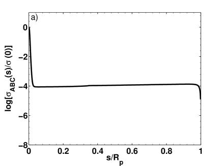
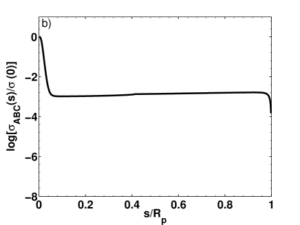
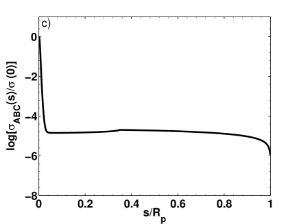
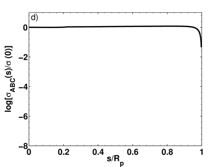
In Fig. 13, we show the combined surface brightness of a fast superwind ($V_{8}=1$) and the bubble that it blows. Panels (a), (b) and (d) correspond to an evaporative bubble, and panel (c) to a bubble for which evaporation has been suppressed. In panels (a), (b) and (c), the cluster mass is $10^{5}$ M_⊙, its radius is $1$-pc and the ISM has a density of $10$-cm^-3. Panels (a) and (b) represent the same bubble at different age. Its relative surface brightness (with respect to that of the wind) decreases as it expands. Since the surface brightness of the superwind goes as $\dot{E}^{2}$ and that of an evaporative bubble goes as $\dot{E}_{38}^{19/35}$ (according to the W77 model), the later effect is enhanced by the increment of $\dot{E}$ by a factor of $\sim 3$ after 3-Myr (Leitherer & Heckman 1995). Similar arguments apply for bubbles without evaporation. The parameters used in panel (a) are the same that were used in panel (e) of fig. 6 in Paper I, where it was shown that the bubble dominates by total X-ray luminosity. Here, we demonstrate that because of the core compactness, the superwind dominates in the X-ray picture. In panel (c), the bubble has the same parameters that in panel (a), but evaporation is not present. The same dynamical model is assumed; thus, the bubble has also the same size, but it is hotter due to the thermalisation process at the reverse shock. Finally, in panel (d) we show the interaction that results when the ISM has a larger density and the cluster has a larger size and a smaller mass. For the assumed parameters, the bubble dominates and the profile is almost flat.

Thus, for compact (when $R_{\rm sc}$ is up to several parsecs) and powerful ($\dot{E}_{38}\gtrsim 1$) clusters, the central emission is dominated by the cluster wind (region A). Around the core, there is a still bright and rapidly decreasing component due to the free wind (region B), but most of the brightness at radii larger than a few times $R_{\rm sc}$ and up to the reverse shock comes from background emission from the superbubble (region C), as the contribution from the free wind becomes negligible in comparison. The rest of the projected emission ($r\geq R_{\rm s}$) comes from the superbubble itself and adopts the profiles shown in Fig. 9 as it evolves with age.

For powerful but extended, or compact but less powerful clusters, the brightness transition from one region to the next is smoother because the central peak produced by the wind emission becomes smaller and wider. Additionally, high ISM densities also contribute to smooth out the transition, since the brightness of region C depends on $n_{0}^{31/35}$ (W77). Only when this circumstances are enhanced, the bubble surface brightness can be comparable to or even higher than that of the superwind.

Nevertheless, there is an additional factor that one must consider. If the evaporation process is inefficient, the bubbles will show limb brightening, but the overall amplitude of their emissions will decrease (see Sections 3.2 and 6.2). In such a case, the corresponding pictures would look similar to those shown in panels (a) and (b) of Fig. 13. This means that if the integration times are not large enough, the observed filling factors will be small, even for young normal clusters (i.e. for clusters that do not qualify as SSCs). This would translate into observing centre brightening or even an apparent spatial disconnection between the X-ray emission and the motion of the outer shell.

6 COMPARISON WITH OBSERVATIONAL DATA

6.1 Nearby clusters

Here, we give a brief summary of the clusters analysed in Paper I. In Table 1, we give the X-ray luminosities obtained from formula (33) for the same sample. The first six columns indicate the observed values. The last three give the results from our analytics. The contributions from hydrogen ($L_{\rm XA,H}$) and metals ($L_{\rm XA,M}$) were separated. The amplitude of the central surface brightness ($A_{\rm AB}$) is given in the last column.

NGC 3603. Using color-magnitude diagrams for the massive stars contained within the core, Sung & Bessell (2004) determined an age of $\tau_{\rm SC}\approx 1\pm 1$ Myr for this cluster. Given the remarkable similarity of the spatial distribution of its stellar content with that of R136, the core of 30 Dor in the LMC (Moffat, Drissen & Shara 1994), we adopt a mass of $1.7\times 10^{4}$ M_⊙ (see Paper I). This corresponds to an energy deposition rate of $1.7\times 10^{38}$ erg s^-1 (Leitherer & Heckman 1995). Moffat et al. (2002) studied the X-ray emission of this cluster and determined a core radius of 0.71-pc. They reported a diffuse X-ray emission of $2\times 10^{34}$ erg s^-1 in the 0.5-10 keV band. Their best-fitted spectra have temperatures $T_{\rm keV}\approx 3.1$ keV for the core and $kT\approx 2.1$ keV for the outer region. They also reported an approximately gaussian-shaped X-ray surface brightness, same that is in agreement with equation (36). The utility of having theoretical estimations for the cumulative X-ray luminosity and surface brightness profiles of star clusters is manifest from that work: its authors used the exterior profile of the diffuse X-ray emission to extrapolate to that of the cluster core, where the high density of point sources made less reliable its direct estimation; even after the use of removal algorithms.

Arches Cluster. The Arches cluster is a very compact and young star cluster. Figer et al. (1999b) determined its age to be $\tau_{\rm SC}\approx 2\pm 1$ Myr. Adopting a low-mass cut-off of 1-M_⊙, they estimated a total stellar mass of $M_{\rm SC}\approx 1.1\times 10^{4}$ M_⊙. This corresponds to an energy deposition rate of $\dot{E}_{38}=1.1$ (Leitherer & Heckman 1995). The cluster radius is $\sim 0.2$-pc (Figer et al. 1999a). Its X-ray emission was studied by Law & Yusef-Zadeh (2004), whom reported a total X-ray luminosity of $(0.5-1.0)\times 10^{35}$ erg s^-1 with $Z=(4-5)\,$ Z_⊙. Just 40 per cent of this is diffuse emission, being the rest due to point sources. As in Paper I, we adopt the Law & Yusef-Zadeh (2004) one-temperature plasma model; thus, $T_{\rm keV}\approx 1.5$ keV.

Quintuplet Cluster. For the 1-pc radius Quintuplet cluster, Figer et al. (1999b) determined a mass of $M_{\rm SC}\approx 8.8\times 10^{3}$ M_⊙ using again a low-mass cut-off of 1-M_⊙. The cluster age has been estimated to be $\tau_{\rm SC}=4\pm 1$ Myr (Figer et al. 1999a). According to the Leitherer & Heckman (1995) evolutionary models, at this age, supernovae have already started to contribute to the wind energy budget. Hence, we adopt $\dot{E}=2.64\times 10^{38}$ erg s^-1. Law & Yusef-Zadeh (2004) studied the X-ray emission of this cluster with the aid of Chandra. Their best fitted spectrum for the cluster core corresponds to a single-temperature solar-metallicity plasma with $T_{\rm keV}=2.4$ keV. They observed an X-ray luminosity of $\sim 1\times 10^{34}$ erg s^-1.

Thanks to the additional physics synthesized in equations (32)-(33), i.e. the direct incorporation of a realistic X-ray emissivity function and the projected temperature, we reach a better agreement between the theoretical and observed luminosities. Their ratios are now reduced to factors $<2$ for the case of the Arches and Quintuplet clusters. A comprehensive interpretation of the X-ray emission of these clusters can be found in Wang et al. (2006). For the case of NGC 3603, the cluster wind X-ray emission accounts for $\sim 30$ per cent of the observed one. This prediction agrees with the results obtained by Li et al. (2006). Their observed and simulated intensity profiles also agree with the general form predicted by equation (36), although each with different indexes $\alpha_{1}$ and $\alpha_{2}$. The later difference is due to the exponential stellar distribution used in their hydrodynamical model. However, our predicted bulk X-ray luminosity is consistent with theirs within a factor of $\sim 2$, since the rapid decrease of the gas density warrants that most of the X-rays come from within the star cluster core and its vicinity. Also, notice that, as they have pointed out, non-CIE effects become important in the supersonic wind region.

The luminosity of the metals surpasses that of hydrogen for the case of the Arches and Quintuplet cluster, whereas for NGC 3603 they are comparable. The effect of compactness and a relative lower temperature can be appreciated in the case of the Arches cluster. This object has a radius just 3.5–5 times smaller than those of the other clusters in the sample, and its temperature is about 1–1.5 keV lower. Comparatively, such differences do not affect too much the X-ray luminosity, but they have an important impact on the surface brightness: the Arches Cluster diffuse X-ray emission is more than 2 orders of magnitude brighter in projection than those of NGC 3603 and the Quintuplet Cluster, albeit its total bolometric X-ray luminosity is just $\sim$3 times larger. This later factor is mainly due to the Arches higher metallicity.

Table 1: Comparison with Nearby Clusters

Object${}^{\,\rm(a)}$	$T_{\rm c}^{\,\rm(b)}$	$R_{\rm sc}^{\,\rm(c)}$	$\dot{E}^{\,\rm(d)}$	$Z^{\,\rm(e)}$	$L_{\rm XA,obs}^{\,\rm(f)}$	$L_{\rm XA,H}^{\,\rm(g)}$	$L_{\rm XA,M}^{\,\rm(h)}$	$A_{\rm AB}^{\,\rm(i)}$
	[keV]	[pc]	$[10^{38}$ erg s${}^{-1}]$	[Z⊙]	[$10^{34}\,$erg s-1]	[$10^{34}\,$erg s-1]	[$10^{34}\,$erg s-1]	[$10^{34}\,$erg s-1 pc-2]
NGC 3603	$3.1\pm 0.7$	0.71	1.7	1	$1.6$	$0.22$	$0.27$	0.80
Arches	$1.5\pm 0.2$	0.20	$1.1$	4	$2.0-4.0$	$0.41$	$3.90$	430
Quintuplet	$2.4\pm 0.5$	1.0	2.6	1	$1.0$	0.71	1.02	1.44

(a): object name; (b): central temperature; (c) star cluster radius, (d): mechanical luminosity; (e) metallicity; (f): observed X-ray luminosity; (g)-(i): predicted X-ray luminosity contributions from hydrogen and metals and amplitude of the central surface brightness. The respective units are indicated between square brackets.

6.2 Bubbles: the case of M 17, magnetically hampered thermal conduction?

M 17 –also known as the Omega Nebula– is powered by a young open cluster with an age of $\sim$1-Myr. The nebula has an overall diameter of $\sim$10–12 pc, and coinciding with it, diffuse X-ray emission has been detected by Chandra (Townsley et al. 2003). Dunne et al. (2003) have studied its properties using a previous data set from a ROSAT observation. Their data sets have similar parameters. The best-fitting spectra is described by a single temperature plasma with $T_{\rm spec}\approx 0.7$ keV, $Z=$Z_⊙ and an rms electron density of $n_{e}\approx 9\times 10^{-2}$ cm^-3. From the observed bubble size (they assumed a filling factor $f_{\rm f}=0.5$), expansion velocity, and stellar content, they derived that $n_{0}\approx$40–60 cm^-3, $\dot{E}_{38}=0.1$ and $t_{6}\approx 0.13$. Using these parameters, they made a comparison with the W77 model. They found that $n_{\rm Cc}\approx$0.2–0.4 cm^-3, $T_{\rm Cc}\approx$5.0–5.6$\times 10^{6}$ K and $L_{\rm XC}\approx$(3–5)$\times 10^{35}$ erg s^-1.

The predicted X-ray luminosity differs by a factor of 120-200 with the observed one, $L_{\rm XC,obs}\approx 2.5\times 10^{33}$ erg s^-1. To explain these discrepancies, Dunne et al. (2003) proposed the total inhibition of the evaporative process by the strong magnetic field (100–500 $\mu$G) that permeates M 17 (Brogan et al. 1999). They required the winds to be significantly clumped and homogeneously mixed in order to match the predicted post-shock temperature ($8\times 10^{7}$ K) with the spectroscopically derived one. An alternative explanation is that while the magnetic field might render the evaporation ineffective, it would not be able to completely avoid it, allowing a smaller fraction of cold gas to mix with the hot bubble interior. In this scenario, the extrapolated central temperature of the bubble would be more similar to the post-shock temperature. In fact, from our analysis, we have that for their value of $T_{\rm spec}$ the almost central temperature of the evaporative bubble is $\approx$2 $\times 10^{7}$ K (see Fig. 11), which makes the discrepancy with the full-evaporative case predicted $T_{\rm Cc}$ even worse.

Nevertheless, if we ignore the particular prescribed dynamical evolution and just consider a general shell-evaporating bubble, we have that $T_{\rm XC}\approx T_{\rm spec}$. In such a case and according to Fig. 11 and equation (55), the value of $T_{\rm XC}$ derived by Dunne et al. (2003) would correspond to a bubble with $T_{\rm Cc}\approx 4$–$5\,T_{\rm XC}$ (the upper bound considers the reverse shock position). This increment of temperature with respect to the one derived from the W77 model has to be compensated by the same decrement in density. Since $L_{\rm X}\propto n_{\rm Cc}^{2}$ this would reduce the predicted X-ray luminosity by a factor of 16–25. If additionally, we consider that the C95 X-ray model overestimates the value of $L_{\rm X}$ by a factor of $\sim$2 (for our derived $T_{\rm Cc}$, see Fig. 7) with respect to the averaged SS00 emissivity, we get a correction factor $\sim$32–50, which would bring $L_{\rm X}$ acceptably close to the observed value. The density near the centre would be also similar to the value derived by Dunne et al. (2003). This would require a decrease of the classical thermal conduction coefficient (Spitzer 1956) of about 2 orders of magnitude. As it was indicated in Section 4, such a drastic change is possible when strong ($>1\mu G$) magnetic fields are involved (see Markevitch et al. 2003 and references therein). Such magnetic fields can hamper the thermal conduction process and establish steeper temperature profiles. Note that this effect is independent from the other observationally deduced parameters ($n_{0},\dot{E}_{38}$ and $t_{6}$) because the bubble size and internal pressure are not affected by the correction factors introduced above (see Section 3).

The previous analysis remarks the relevance of the projected temperature as a diagnostic tool, as well as the necessity of a broader-scope assessment of the thermal conductivity efficiency for the case of bubbles.

7 SUMMARY

Our findings and their immediate consequences are:

1. A new and simple star cluster wind model has been developed. Assuming a polytropic equation of state we reproduced the effect of radiative cooling on the hydrodynamical profiles, in consonance with previous numerical calculations. Moreover, the door has been left open to further applications like the parameterization of other effects, the constraining of the parameter space through threshold lines and the analysis of other branches of the solution.

2. The superwind X-ray luminosity has been calculated using a realistic X-ray emissivity that allowed the separation of the contributions from hydrogen and metals. Good agreement was obtained when we compared with observational data. Also, transformation laws to include very general emissivity functions and completely characterize the global properties of the models have been given.

3. We have calculated the corresponding surface brightness and shown that although the adiabatic superwind model predicts a very extended X-ray emitting volume, the X-ray bright super star cluster cores are expected to be observed surrounded by compact and faint haloes (if their bubbles are not considered). The weighted temperatures associated to the cluster cores were also obtained.

4. An analogue to the C95 X-ray luminosity model has been obtained considering a realistic emissivity function. The model is independent of the assumed dynamical evolution for bubbles with $R_{\rm s}/R_{\rm p}\leq 0.4$. Significant deviations were observed with respect to the C95 model when $T_{\rm Cc}\rightarrow 10^{6}$ K. It was also found that for under-developed bubbles (when the ratios of the reverse and leading shocks are $>0.4$) with extrapolated central temperatures on this range, the bubble X-ray luminosity can be drastically reduced by the relative closeness of the reverse and main shock positions.

5. The X-ray surface brightness of evaporative bubbles has been obtained in terms of elementary functions by introducing a pseudo-triangle approximation. It has been shown that limb-brightening, flat and limb-darkening modes are all possible according to the value of the central temperature. Because we have separated the self-similar spatial profiles from what we call an intensity amplitude and a weighting emissivity factor, they are valid for all evaporative models based on the classical thermal conduction theory.

6. It has been demonstrated that moderately hot, well-developed shell-evaporating bubbles ($T_{\rm Cc}\approx 10^{6}$ K) have X-ray weighted temperatures somewhat similar to their central ones ($T_{\rm XC}\sim 0.5$–$1\,T_{\rm Cc}$) in major fractions of their projected areas. On the other hand, very hot bubbles ($T_{\rm Cc}\ga 10^{7}$ K) are expected to have point-wise projected temperatures of about 0.25–0.50$\,T_{\rm Cc}$. Nevertheless, the hottest bubbles can still have projected temperatures of the order of $1$ keV. Since $T_{\rm XC}$ is a measure of the temperature at which the plasma is emitting the most, it is important to account for the difference between this and the actual temperature at different radii. This can be also useful to evaluate the efficiency of the thermal evaporation process.

7. We also studied the case of when the evaporative process is totally inhibited. In this case, the bubbles have very hot interiors since their temperatures are similar to the post-shock temperature. Their surface brightness was also obtained.

8. We have assembled the X-ray brightness models and presented a very descriptive and comprehensive X-ray picture of the interaction of the superwind with the ISM.

All these tools are expected to be helpful at the time of comparing the models with the observations.

8 ACKNOWLEDGMENTS

We wish to thank D. Strickland & I. Stevens for kindly providing their X-ray emissivity tables. Our gratitude is also extended to the anonymous referees whose very valuable suggestions helped to greatly improve this paper. This work has been supported by CONACYT-México research grants 60333 and 82912. This paper was prepared with the help of the MNRAS LaTeXstyle and class files.

Appendix A SUPERWINDS X-RAY LUMINOSITY

It is convenient to initially adopt a constant X-ray emissivity $\Lambda_{\rm X}=\Lambda_{0}$ and express the integral (24) in terms of the velocity instead of the radius. The related quantities will be labeled with the subindex ’0’.

A.1 Initial formalism

Region A

Substituting (24) and (1) in (16) and introducing the variables $x={U^{\prime}}/{U}$, $z=-3(2\eta+1)U$ and $f=(1-zx)$ we get that $L_{\rm XA0}=X_{A}(I_{1}+I2)$ with

$$I_{1}=\frac{1}{2}U^{3/2}\int_{0}^{1}\Lambda_{0}x^{1/2}f^{-\frac{10}{3}}{\rm{d}}x,$$ (58)

$$I_{2}=-2(2\eta+1)U^{5/2}\int_{0}^{1}\Lambda_{0}x^{3/2}f^{-\frac{13}{3}}{\rm{d}}x,$$ (59)

and

$$X_{\rm A}=\frac{D_{\rm 1P}^{5}\dot{E}^{2}}{\pi\mu_{\rm n}^{2}V_{\rm\infty P}^{6}R_{\rm sc}}.$$ (60)

In what follows f will be called a ”base”, for reasons that will be evident in brief. The above integrals can be expressed in terms of Gauss hypergeometric functions (see for instance, Whittaker & Watson 1996 and Lebedev 1972):

$${}_{2}F_{1}(a,b;c;z)=\frac{\Gamma(c)}{\Gamma(b)\Gamma(c-b)}\int_{0}^{1}x^{b-1}(1-x)^{c-b-1}(1-zx)^{-a}{\rm{d}}x,$$ (61)

where $\Gamma$ is the Gamma function. It follows that $a_{1}={10}/{3},\,b_{1}={3}/{2},c_{1}=b_{1}+1$ and $a_{2}=a_{1}+1,\,b_{2}=b_{1}+1,\,c_{2}=b_{1}+2$. Then,

$$L_{\rm XA0}=X_{\rm A}\Lambda_{0}U^{3/2}\left[\frac{1}{2b_{1}}F_{1}-2\frac{(2\eta+1)}{b_{1}+1}UF_{2}\right].$$ (62)

Above, to simplify the notation we have used the label of each family of indexes to make reference to the corresponding hypergeometric functions: $F_{1}={{}_{2}F_{1}(a_{1},b_{1};c_{1};z)}$ and $F_{2}={{}_{2}F_{1}(a_{2},b_{2};c_{2};z)}$. We shall keep this custom in what follows. Each $U\in\left[0,{1}/({2\eta+1})\right]$ yields the value of $L_{\rm XA0}$ at the radius indicated by (16). Alternatively, one may use the temperature $T=T_{\rm c}(1-U)\in[T_{\rm c},T_{\rm sc}]$ as the independent variable.

For $\eta=\frac{3}{2}$, the total luminosity can be approximated by

$$L_{\rm XA0,total}=\left(1.12\times 10^{34}\mbox{erg s${}^{-1}$}\right)\frac{\Lambda_{\rm X,-23}(\overline{T},Z)\dot{E}_{38}^{2}}{R_{\rm sc,pc}V_{8}^{6}}=\left(9.63\times 10^{33}\mbox{erg s${}^{-1}$}\right)\frac{\Lambda_{\rm X,-23}(\overline{T},Z)\dot{E}_{38}^{2}}{R_{\rm sc,pc}T_{\rm keV}^{3}},$$ (63)

where we evaluated (62) at $U=U_{\rm sc}$ and took $\Lambda_{0}=\Lambda_{\rm X}(\overline{T},Z)$. The value of the emissivity function for the reference temperature $\bar{T}$ is taken from the SS00 tables.

Region B

For quasi-adiabatic superwinds, $\eta\approx\frac{3}{2}$ for $r\geq R_{\rm sc}$ and $U\in[U_{\rm sc},1)$. In principle, superwinds with $V_{\rm\infty P}$ of the order of 1000 km s^-1 have very extended X-ray envelopes, since the connection between temperature and radius is given by

$$R=D_{2}\left(1-\frac{T}{T_{\rm c}}\right)^{-1/4}\left(\frac{T}{T_{\rm c}}\right)^{-\eta/2}.$$ (64)

Nevertheless, the outermost layers meagerly contribute to the luminosity, since most of the emission from this region comes from a compact shell of gas around the star cluster. Thus, it suffices to estimate the external X-ray luminosity and surface brightness of quasi-adiabatic superwinds because those of superwinds in the radiative regime would be alike, despite the effective cropping of their X-ray emitting envelopes by radiative cooling. Introducing the variables $x={U^{\prime}}/{U_{l}}$ and $z=U_{l}$ we find that

$$L_{\rm XB0}=X_{\rm B}\Lambda_{0}U_{l}^{-3/4}\left[\frac{\eta}{2(b_{4}+1)}UF_{3}-\frac{1}{4b_{4}}F_{4}\right]_{U_{l}=U_{\rm sc}}^{U_{l}=U},$$ (65)

with $a_{4}=-{\eta}/{2},\,b_{4}={3}/{4},\,c_{4}=b_{4}+1$ and $a_{3}=a_{4}+1,\,b_{3}=b_{4}+1,c_{3}=b_{4}+2$ and

$$X_{\rm B}=\frac{\dot{E}^{2}}{\pi D_{2}\mu_{\rm n}^{2}R_{\rm sc}V_{\rm\infty P}^{6}}.$$ (66)

The velocity at the cut-off radius is $U_{\rm cut}=\left(1-{T_{\rm cut}}/{T_{\rm c}}\right)$. For fast winds $U_{\rm cut}\approx 1$. Accordingly, we can replace the hypergeometric functions with their asymptotic limits using the Euler beta function and the identity $\Gamma(v)\Gamma(1-v)={\pi}/{\sin(\pi v)}$:

$$\lim_{z\rightarrow 1^{-}}\,{}_{2}F_{1}(a,b;c;z)=\frac{\Gamma(c)\Gamma(c-a-b)}{\Gamma(c-b)\Gamma(c-a)}=\frac{\Gamma(c)}{\Gamma(c-a)\Gamma(a)}\frac{\pi}{\sin(\pi a)}.$$ (67)

Then, for $\eta=\frac{3}{2}$, $F_{3}$ and $F_{4}$ can be substituted by

$$\begin{array}[]{ll}\lim_{z\rightarrow 1^{-}}F_{3}&=2^{-3/2}\pi,\\ \lim_{z\rightarrow 1^{-}}F_{4}&=3(2^{-3/2}\pi).\end{array}$$ (68)

Combining these equations with (65) we obtain that

$$L_{\rm XB0}\approx\frac{1}{4}L_{\rm XA0}.$$ (69)

This luminosity comes from a very large volume. Since radiative cooling brings the X-ray cut-off temperature closer to $R_{\rm sc}$, the actual emitting region is more compact. Consequently, the contribution of the free wind is smaller. This conclusion does not change when the SS00 emissivity is considered, as can be shown using the transformation laws given below and consulting the numerical results of Paper I. Because of this, we shall focus on region A, but providing a general formalism to account for region B if it is desired.

A.2 Transformation laws

Before proceeding any further we shall establish laws for transforming equations (62) and (65) such that they can handle more general X-ray emissivity functions with explicit dependence on metallicity. For this reason, $\Lambda_{0}$ was kept intentionally inside of the integrals (58) and (59). These laws can be used to calculate other integral properties of the superwind such as its mass and energy within a certain volume. The laws also apply for bubbles.

Let $a^{\prime}$, $b^{\prime}$, $\alpha$ and $\Lambda_{a^{\prime}}$,$\Lambda_{b^{\prime}}$, $\Lambda_{\rm\alpha}$ be arbitrary constants. The following transformations apply to (58) and (59) and similar integrals like those for region B and C:

Law I: if $\Lambda_{\rm X}=\Lambda_{\rm\alpha}f^{\alpha}$ then the transformation $a\rightarrow a-\alpha$ applies for the leading index and $\Lambda_{0}\rightarrow\Lambda_{\rm\alpha}$ for each term.

Law II: if $\Lambda_{\rm X}=\Lambda_{\rm\alpha}f^{\prime a^{\prime}}$ with $f^{\prime}=(1-xz^{\prime})$ and $z^{\prime}$ independent from $z$, then ${}_{2}F_{1}\rightarrow F_{\rm A}$, where $F_{\rm A}$ is the Appell hypergeometric function which has two bases $(f,f^{\prime})$ and two leading indexes $(a,-a^{\prime})$:

$$F_{\rm A}(a,-a^{\prime},b;c;z,z^{\prime})=\frac{\Gamma(c)}{\Gamma(b)\Gamma(c-b)}\int_{{}_{0}}^{1}x^{b-1}(1-x)^{c-b-1}f^{-a}f^{a^{\prime}}{\rm{d}}x.$$ (70)

Again, $\Lambda_{0}\rightarrow\Lambda_{a^{\prime}}$ applies for each term.

Law III: if $\Lambda_{\rm X}=\Lambda_{b^{\prime}}x^{b^{\prime}}$ then we need to use first the transformations $b\rightarrow b+b^{\prime}$ and $c\rightarrow c+b^{\prime}$ and then $\Lambda_{0}\rightarrow{\Gamma(c-b)\Gamma(b)}/{\Gamma(c)}\Lambda_{b^{\prime}}$ for each term.

Since $a$, $b$ and $c$, $\alpha$ and $a^{\prime}$ are mutually independent, we can apply the three laws simultaneously if it is required. Because all the hydrodynamical variables are functions of $f$, $f^{\prime}$ and $x$ (or $u$) these laws suffice to calculate any integral property.

In this paper, we used them to calculate the X-ray emission assuming a realistic $\Lambda_{\rm X}$. This was done as follows: considering the more general case $\Lambda_{\rm X}=\sum\Lambda_{\rm\alpha}T^{\alpha}$, where $\Lambda_{\rm\alpha}$ are constants that can scale with metallicity (see Table 3) and each $\alpha\in[-4,4]$, we applied Law II to the quantity between square brackets in (62) and proceeded to expand it rationally around $U=0$ (after dividing by $T_{\rm c}^{\alpha}$) recurring to admissible hypergeometric transformations (see the references in Section A.1). We used a (0,2) Padé approximant to make the rational approximation around 0. This warrants a coincidence of up to the second order with the Taylor expansion of the original function and provides an accurate approximation for large values of $\eta$, since $U_{sc}=1/(2\eta+1)$. To account for small values of $\eta$ and the effect of the exponents of the power laws, we later introduced two curvature matching filters. The next expression valid on $U\in[0,{1}/({2\eta+1})]$ was obtained:

$$\mathcal{F_{A}}(\eta,\alpha,U)=\frac{350\left(1-U\right)^{\frac{\alpha}{30}}\left[1+\frac{\eta^{2}(8\eta+1)}{5(2\eta+1)}U^{2}\right]^{4/10}}{9\left(\frac{350}{3}+\phi_{1}U+\phi_{2}U^{2}\right)},$$ (71)

where

$$\phi_{1}(\eta,\alpha)=70(\alpha+28\eta+14),$$ (72)

and

$$\phi_{2}(\eta,\alpha)=17\alpha^{2}+\alpha(501+952\eta)+9528\eta(1+\eta)+2382.$$ (73)

The quantity between parenthesis on the numerator of equation (71) is a matching filter of the form $(T/T_{\rm c})^{b}$ that corrects for the curvature introduced by $\alpha$. Likewise, the quantity between square brackets is a filter of the form $[1-g(\eta)U^{b}]^{c}$ that corrects for the curvature introduced by $\eta>0.3$. The filter parameters where obtained by minimization of the relative error of the approximation. For the SS00 emissivity function we always obtain an accuracy better than 5 per cent. In general, the same applies for all emissivity functions with $\alpha\in[-4,4]$ provided that $\eta\geq 3/2$. This ensures a good coverage of the radiative wind case. For the most extreme combination of parameters we are considering, i.e. for $\eta\approx 0.3$ and $\alpha\approx 4$, the accuracy is $\sim 15$ per cent.

From equation (71) and Law II, it follows that the cumulative X-ray luminosity is

$$L_{\rm XA}(\eta,\{\alpha\},U)=X_{\rm A}U^{3/2}\sum_{\rm\alpha}\mathcal{F_{A}}(\eta,\alpha,U)\Lambda_{\rm\alpha}T_{\rm c}^{\alpha},$$ (74)

where $X_{\rm A}$ is given by equation (60).

Appendix B EVAPORATIVE BUBBLES SURFACE BRIGHTNESS

Just for convenience, we assume initially an X-ray emissivity function with a power-law dependence on the temperature, $\Lambda_{\rm X}=\Lambda_{\rm\alpha}T^{\alpha}$, where the constant $\Lambda_{\rm\alpha}$ might or might not scale with metallicity. We then express all the relevant variables of the evaporative model (Section 3) in terms of the ratio of the point-wise temperature $T_{\rm c}$ to the central value: $\vartheta=T_{\rm c}/T_{\rm Cc}$. From equations (46) and (47) one has that $r=R_{\rm p}(1-\vartheta^{5/2})$, $n_{\rm C}=n_{\rm Cc}\vartheta^{-1}$, $s=R_{\rm p}(1-\vartheta_{s}^{5/2})$, $s_{\rm cut}=R_{\rm p}(1-\vartheta_{\rm cut}^{5/2})$ and $R_{\rm s}=R(1-\vartheta_{\rm Rs}^{5/2})$. The surface brightness can then be separated into a temporal amplitude, $A_{\rm C}$; a weighted emission factor, $\lambda_{\alpha}$; and a spatial profile $\Theta(s)$ –between two reference points $s_{\rm i}$ and $s_{\rm f}$– that implicitly but slowly changes with time, such that $\sigma_{\rm C}=A_{\rm C}(t)\lambda_{\rm\alpha}\Theta(\vartheta_{\rm i};\vartheta_{{f}})$ with

$$A_{\rm C}(t)=2R_{\rm p}n_{\rm Cc}^{2}\Lambda_{1},$$ (75)

$$\lambda_{\rm\alpha}=\frac{\Lambda_{a}T_{\rm Cc}^{\alpha}}{\Lambda_{1}}=\Lambda_{\alpha,-23}T_{\rm Cc}^{\alpha},$$ (76)

and

$$\Theta(\vartheta_{s},\alpha;\vartheta_{{i}},\vartheta_{{f}})=\int_{\vartheta_{{i}}}^{\vartheta_{\rm f}}\frac{\left(\frac{5}{2}\right)\vartheta^{\alpha}(\vartheta^{2}-\vartheta^{-1/2})}{\sqrt{(\vartheta_{\rm s}^{5/2}-\vartheta^{5/2})(2-\vartheta_{\rm s}^{5/2}-\vartheta^{5/2})}}{\rm{d}}\vartheta,$$

(77)

where $\Lambda_{1}=10^{-23}$ erg cm³ s^-1. Notice that $\vartheta_{\rm i}>\vartheta_{\rm f}$ because the bubble temperature gradient is negative.

The integral above can be expressed in terms of Appell hypergeometric functions $F_{\rm A}$

$$\Theta(\vartheta_{s},\alpha;\vartheta_{\rm i},\vartheta_{\rm f})=\left[\frac{\vartheta^{\frac{1}{2}+\alpha}}{(2\vartheta_{\rm s}^{5/2}-\vartheta_{\rm s}^{5})^{1/2}}\right.\left.\left(\frac{\vartheta^{5/2}}{b_{1}+1}F_{\rm A2}-\frac{1}{b_{1}}F_{\rm A1}\right)\right]_{\vartheta=\vartheta_{\rm i}}^{\vartheta=\vartheta_{\rm f}},$$ (78)

where $b_{1}=\frac{1}{5}+\frac{2}{5}\alpha$, $F_{\rm A1}=F_{\rm A}[{1}/{2},{1}/{2},b_{1};b_{1}+1;{\vartheta^{5/2}}/{\vartheta_{\rm s}^{5/2}},{\vartheta^{5/2}}/({2-\vartheta_{\rm s}^{5/2}})]$, and similarly, $F_{\rm A2}=F_{\rm A}[1/2,1/2,b_{1}+1;b_{1}+2;{\vartheta^{5/2}}/{\vartheta_{\rm s}^{5/2}},{\vartheta^{5/2}}/({2-\vartheta_{\rm s}^{5/2}})]$. For a single power law X-ray emissivity, the surface brightness spatial profile in terms of the temperature is

$$\sigma_{\rm C}(\vartheta,t)=A_{\rm C}(t)\lambda_{\rm\alpha}\Theta[\vartheta_{\rm s},\alpha;\min(\vartheta_{\rm s},\vartheta_{R_{\rm s}}),\vartheta_{\rm cut}].$$ (79)

In terms of the projected radius $s$ we have that

$$\sigma_{\rm C}(s,t)=A_{\rm C}(t)\lambda_{\rm\alpha}S_{\rm C}[s,\alpha;\max(s,R_{\rm s}),R_{\rm cut}].$$ (80)

In the last formula, we used the transformations indicated at the beginning of this appendix to go back to the spatial coordinate; thus, $\Theta(\vartheta_{\rm s}...\vartheta_{ref})\rightarrow S_{\rm C}(s...s_{Xref})$. For the singular cases –when both arguments of the minimum or maximum function are the same– we define $\min(a,a)=\max(a,a)=a$. For a realistic emissivity expanded as a power series, equation (79) immediately transforms into

$$\sigma_{\rm C}(\vartheta_{\rm s},t)=\left\{\begin{array}[]{ll}A_{\rm C}(t)\displaystyle{\sum_{\alpha,\vartheta_{\rm i},\vartheta_{\rm f}<\vartheta_{\rm R_{\rm s}}}^{\vartheta_{\rm f}=\vartheta_{\rm cut}}}\lambda_{\alpha}\Theta[\vartheta_{\rm s},\alpha;\min(\vartheta_{\rm i},\vartheta_{\rm R_{\rm s}}),\vartheta_{\rm f}],\mbox{if $s\leq R_{\rm s}$;}\\ A_{\rm C}(t)\displaystyle{\sum_{\ \alpha,\vartheta_{\rm i},\vartheta_{\rm f}<\vartheta_{s}}^{\vartheta_{\rm f}=\vartheta_{\rm cut}}}\lambda_{\alpha}\Theta[\vartheta_{\rm s},\alpha;\min(\vartheta_{\rm s},\vartheta_{\rm i}),\vartheta_{\rm f}],\mbox{otherwise;}\end{array}\right.$$ (81)

here, $\vartheta_{\rm i}$ and $\vartheta_{\rm f}$ are respectively the upper and lower temperature limit for which the power law with index $\alpha$ is valid.

Equations (78)-(81) and their analytical properties are enough to calculate the surface brightness spatial profile. Nevertheless, we still need closed algebraic formulas for evaluating them swiftly and accurately. They are obtained in the next appendix.

Appendix C HYPERGEOMETRIC PSEUDO-TRIANGLES

Consider the negative of the quantity between the big parenthesis in equation (78) evaluated separately at the end-points while considering a single power-law emissivity and ignoring temporally the reverse shock position

$$\mathcal{F_{\rm c}}(\vartheta,\vartheta_{\rm s};\alpha)=\left.\left(\frac{5}{1+2\alpha}F_{\rm A1}-\frac{5}{6+2\alpha}\vartheta^{5/2}F_{\rm A2}\right)\right|_{\vartheta_{s}}^{\vartheta_{\rm f}},$$ (82)

where $\vartheta_{\rm f}$ is a reference temperature below $\vartheta_{\rm s}$ ($r_{\rm f}>s$). For a single power law $r_{\rm f}=R_{\rm cut}$. We get then a pair of functions that we express in terms of the variable $\tau=\vartheta^{5/2}_{\rm s}=\left(1-{s}/{R_{\rm p}}\right)$

$$\mathcal{F_{C,H}}(\tau;\alpha)=\begin{array}[]{ll}\frac{5}{1+2\alpha}F_{\rm A1}\left(",1,\frac{\tau}{2-\tau}\right)-\frac{5}{6+2\alpha}\tau F_{\rm A2}\left(",1,\frac{\tau}{2-\tau}\right),\end{array}$$ (83)

$$\mathcal{F_{C,C}}(\tau,\tau_{\rm f};\alpha)=\begin{array}[]{ll}\frac{5}{1+2\alpha}F_{\rm A1}\left(",\frac{\tau_{\rm f}}{\tau},\frac{\tau_{\rm f}}{2-\tau}\right)-\frac{5}{6+2\alpha}\tau_{\rm f}F_{\rm A2}\left(",\frac{\tau_{\rm f}}{\tau},\frac{\tau_{\rm f}}{2-\tau}\right).\end{array}$$ (84)

At $\tau=\tau_{\rm f}$, the two functions above take the same value, since $\tau_{\rm f}$ is the cut-off value for the emission with temperature slope $\alpha$. By symmetry, the functions in question also take the same value at the limit $\tau\rightarrow 1^{-}$. The simplest way to prove this is to find the primitive function of the integrand in equation (77) in spatial coordinates and carry out a comparison with equation (78). Proceeding this way, one can find that

$$\mathcal{F_{C,H}}(1^{-};\alpha)=\mathcal{F_{C,C}}(1^{-},\tau_{\rm f};\alpha)=\frac{1}{b_{1}}=\frac{5}{1+2\alpha}.$$ (85)

Thus, equations (83) and (84) form a closed path: a pseudo-triangle. This is per se a very interesting property both from the physical and mathematical point of view, which complete study we reserve for a later time. Here, we give just a brief discussion that is general enough to solve the (super-) bubble surface brightness problem. The actual shape of the triangles depends on $\tau_{\rm f}^{2/5}=\vartheta_{\rm f}={T_{\rm f}}/{T_{\rm Cc}}$. For $T_{\rm Cc}\ga 10T_{\rm f}$ there is practically no curvature, whereas for $T_{\rm Cc}\approx T_{\rm f}$ the catheti are deformed (Fig. 14). For the range of $\alpha$ that we are considering (see Table 3), a series expansion shows that the hypotenuse is always, for any practical purpose, a straight line. A convenient point that one can use to trace it is $0^{+}$. There, the second term in (83) vanishes. After working with its integrand, the first term on (83) can be reduced to $(1/b_{1})\sqrt{\pi}\Gamma(b_{1}+1){}_{1}F_{2}[1/2,b;b+1/2;\tau/(2-\tau)]/\Gamma(b_{1}+1/2)$. At the limit $\tau\rightarrow 0^{+}$, the previous Gauss hypergeometric function reduces to unity. As a consequence $\mathcal{F_{C,H}}$ takes the value

Figure 14: Hypergeometric pseudo-triangles. The hypothenuse $\mathcal{F_{C,H}}$ is given by equation (83). The function $\mathcal{F_{C,C}}$, that corresponds to the catheti, is given by equation (84). Top: $T_{\rm Cc}=1.68\times 10^{7}$ K, $\alpha=0$ (Chu et al. 1995 model). Bottom: $T_{\rm Cc}=6.4\times 10^{6}$ K, $\alpha={1}/{2}$ (Bremsstrahlung). Solid lines: actual hypergeometric functions. Dashed lines: pseudo-triangle approximations.

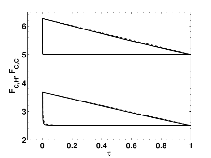
$$\mathcal{F_{C,H}}(0;\alpha)=\sqrt{\pi}\frac{\Gamma(\frac{1+2\alpha}{5})}{\Gamma(\frac{1+2\alpha}{5}+\frac{1}{2})}.$$ (86)

The function $G(x)={\Gamma(x)}/{\Gamma(x+{1}/{2})}$ can be approximated on the interval $(-{1}/{2},1)$ by the following (1,2) Padé approximant around 0:

$$G(x)=\frac{\Gamma(x)}{\Gamma(x+\frac{1}{2})}\approx\frac{[\pi^{2}+3\ln(4)^{2}]x+6\ln(4)}{\sqrt{\pi}x\{[\pi^{2}-3\ln(4)^{2}]x+6\ln(4)\}}.$$ (87)

For the case under study, when $x$ falls out of this range, it can always be mapped back using the relation $\Gamma(x+1)=x\Gamma(x)$. The equation of the line that traces the hypothenuse is

$$\mathcal{F_{C,H}}(\tau;\alpha)\approx\begin{array}[]{ll}\sqrt{\pi}G\left(\frac{1+2\alpha}{5}\right)+\left[\frac{5}{1+2\alpha}-\sqrt{\pi}G\left(\frac{1+2\alpha}{5}\right)\right]\tau.\end{array}$$ (88)

The slope of this line, $m$, just depends on $\alpha$. For $\alpha=0$, it reduces to $m(0)\approx-{\pi}/{2}=-\mbox{arccsc}(1)=-\mbox{arcsin}(1^{-1})$. This hints that a secant-like approximation can be used to obtain an expression for the catheti. Because we have a closed path, a single secant approximation on $\tau\in[\tau_{\rm f},1]$ just recovers the expression for the hypothenuse. We consider a multi-secant approximation of the form $\sin(\beta)\approx\sin\{[\mathcal{F_{C,C}}-5/(1+2\alpha)]/(1-\tau)\}=g(\tau)$, where $g(\tau)$ accounts for the variable angle $\beta$ that the catethi subtend with the negative direction of the $\tau$-axis. Consistency requires the closure of the path to be conserved; thus, it is obligatory that $g(\tau_{f})=\sin(-m)$. Taking into account the catheti dependence on $\tau_{\rm f}/\tau$, $g(\tau)$ can be written as $g(\tau)=h(\tau_{\rm f}/\tau)\sin(-m)$, where $h(\tau_{\rm f}/\tau)$ is a function that satisfies $h(1)=1$. Many of such functions exist, for instance, any of the form $h(\tau_{\rm f}/\tau)/h(1)$. Equation (84) diverges as $\sim\tau_{\rm f}/\tau$ as $\tau\rightarrow 0$, so we use $h(\tau_{\rm f}/\tau)=\tau_{\rm f}/\tau$. This is equivalent to a first order approximation. It suffices for the present discussion. Thus, the expression for the catheti is

$$\mathcal{F_{C,C}}(\tau,\tau_{\rm f};\alpha)\approx\left\{\begin{array}[]{ll}\frac{5}{1+2\alpha}+(1-\tau)\mbox{arcsin}\left[\frac{\tau_{\rm f}}{\tau}\sin(-m)\right],\mbox{if abs$(m)\leq\frac{\pi}{2}$;}\\ \frac{5}{1+2\alpha}+(1-\tau)\left\{\frac{\tau_{\rm f}}{\tau}\pi-\mbox{arcsin}\left[\frac{\tau_{\rm f}}{\tau}\sin(-m)\right]\right\},\mbox{otherwise;}\end{array}\right.$$ (89)

where the last case separation is necessary to take the correct value of the arcsin function, specially when machine-evaluated. For a single power law emissivity, equations (78)-(79) and the expressions for the hypotenuse and the catheti give the next approximation for the spatial profile as a function of the normalised temperature

$$\begin{array}[]{ll}\Theta_{\triangle}(\vartheta_{\rm s},\alpha;\xi_{\rm f},\xi_{\rm i})=(2\vartheta_{\rm s}^{\frac{5}{2}}-\vartheta_{\rm s}^{5})^{-1/2}\left[\xi^{\frac{1}{2}+\alpha}\mathcal{F_{C,C}}(\vartheta_{\rm s}^{5/2},\xi^{5/2};\alpha)\right]_{\xi_{\rm i}=\vartheta_{\rm cut}}^{\xi_{\rm f}=\min(\vartheta_{\rm s},\vartheta_{R_{\rm s}})},\end{array}$$ (90)

where the dummy variable $\xi$ is meant to be evaluated at the indicated limits as the result of an integral would and $\min(\vartheta_{\rm s},\vartheta_{R_{\rm s}})$ brings the reverse shock position back into the game. In terms of the projected radius, the profile is

$$\begin{array}[]{ll}S_{\rm C\triangle}(s,\alpha;\xi_{\rm f},\xi_{\rm i})=\left[1-\left(\frac{s}{R_{\rm p}}\right)^{2}\right]^{-1/2}\left[(1-\xi)^{\frac{1+2\alpha}{5}}\mathcal{F_{C,C}}[1-s,1-\xi;\alpha]\right]_{\xi_{\rm i}=\frac{s_{\rm cut}}{R_{\rm p}}}^{\xi_{\rm f}=\max(\frac{s}{R_{\rm p}},\frac{R_{\rm s}}{R_{\rm p}})}.&\end{array}$$ (91)

The expression that corresponds to a realistic emissivity (see Fig. 15 and Table 3) parameterized as piecewise continuous power laws is obtained from equation (81)

$$\sigma_{\rm C}(\vartheta_{\rm s},t)=\left\{\begin{array}[]{ll}A_{\rm C}(t)\displaystyle{\sum_{\alpha,\vartheta_{\rm i},\vartheta_{\rm f}<\vartheta_{R_{\rm s}}}^{\vartheta_{\rm f}=\vartheta_{\rm cut}}}\lambda_{\alpha}\Theta_{\triangle}[\vartheta_{\rm s},\alpha;\min(\vartheta_{\rm i},\vartheta_{R_{\rm s}}),\vartheta_{\rm f}],&\mbox{if $s\leq R_{\rm s}$;}\\ A_{\rm C}(t)\displaystyle{\sum_{\ \alpha,\vartheta_{\rm i},\vartheta_{\rm f}<\vartheta_{\rm s}}^{\vartheta_{\rm f}=\vartheta_{\rm cut}}}\lambda_{\alpha}\Theta_{\triangle}[\vartheta_{\rm s},\alpha;\min(\vartheta_{\rm s},\vartheta_{\rm i}),\vartheta_{\rm f}],&\mbox{otherwise;}\end{array}\right.$$ (92)

or, in terms of $s$

$$\sigma_{\rm C}(s,t)=\left\{\begin{array}[]{ll}A_{\rm C}(t)\displaystyle{\sum_{\alpha,s_{\rm i},s_{\rm f}>R_{\rm s}}^{s_{\rm f}=R_{\rm cut}}}\lambda_{\alpha}S_{\rm C\triangle}[s,\alpha;\max(s_{\rm i},R_{\rm s}),s_{\rm f}],&\mbox{if $s\leq R_{\rm s}$;}\\ A_{\rm C}(t)\displaystyle{\sum_{\ \alpha,s_{\rm i},s_{\rm f}>s}^{s_{\rm f}=R_{\rm cut}}}\lambda_{\alpha}S_{\rm C\triangle}[s,\alpha;\max(s,s_{\rm i}),s_{\rm f}],&\mbox{otherwise.}\end{array}\right.$$ (93)

These formulae give the surface brightness spatial profile for all evaporative bubble models. They can be also used to calculate the weighted temperature, as we show in Section 3.3.

Appendix D AUXILIARY TABLES AND FIGURES

Table 2: LIST OF RELEVANT SYMBOLS

Symbol (page)	Meaning	Symbol (page)	Meaning
indexes ’A’, ’B’ & ’C’	properties at regions A,B and C, respectively	index ’X’	a property in the X-ray band
index ’$\rm sc$’	values at $r=R_{\rm sc}$	index ’$\rm c$’	central values
index ’H’	contribution from hydrogen	index ’M’	contribution from metals
index ’7’	temperature in units of $10^{7}$ K	$\Pi_{*}$	$\Pi_{*}=\{R_{\rm sc},q_{\rm e},\{q_{\rm m},V_{\infty P}\}\}$
$A$ (6)	surface brightness amplitude	$\dot{E}(3)$	mechanical luminosity
$\dot{E}_{38}$ (2,5)	$\dot{E}$ in units of $10^{38}$ erg s-1	$F$ (18)	Gauss hypergeometric function ${}_{2}F_{1}$
$F_{\rm A}$ (19)	Appell hypergeometric function	$k$ (3)	Boltzmann constant
$K$ (3)	polytropic proportionality constant	$L_{\rm X}$ (5)	cumulative X-ray luminosity
$\dot{M}(3)$	mass deposition rate	$n$ (5)	particle number density
$n_{0}$ (9)	ISM particle number density	$P(3)$	pressure
$q_{\rm m}$ (3)	mass deposition rate per unit volume	$q_{\rm e}(3)$	energy deposition rate per unit volume
$r$ (3)	radial coordinate	$r_{\rm d}(6)$	angular diameter distance
$R$ (3)	a normalised radius: $R=r/R_{\rm sc}$	$R_{\rm sc}(3)$	star cluster radius
$R_{\rm sc,pc}$ (2,5)	star cluster radius in parsecs	$R_{\rm cut}$ (6)	X-ray cut-off radius
$R_{\rm p}$ (9)	principal shock position	$R_{\rm s}$ (9)	reverse shock position
$s$ (6,7)	projected radius	$S$ (10,21)	surface brightness spatial profile
$t$ (9)	time	$t_{6}$(2,9)	time in Myr
$T$ (3)	temperature	$T_{\rm X}$ (7)	X-ray weighted temperature
$T_{\rm keV}$ (4,5)	superwind central temperature in keV	$T_{\rm Rs}$ (10)	temperature at $R_{\rm s}^{+}$
$T_{\rm cut}$ (6)	X-ray cut-off temperature	$T_{\rm spec}$ (7)	X-ray spectroscopic temperature
$u$ (3)	velocity	$U$ (3)	squared velocity: $u^{2}$
$V_{\rm\infty A}(3)$	adiabatic terminal speed	$V_{\rm\infty P}$ (3)	polytropic terminal speed
$V_{8}$ (2,5)	$V_{\rm\infty P}$ in units of 1000 km s-1	$V_{\rm sc}$ (3)	star cluster volume
$X$ (5)	X-ray luminosity scaling factor	$Z$ (5)	metallicity
$\alpha$ (5)	X-ray emissivity temperature slope	$\gamma$ (3)	adiabatic index
$\Gamma$ (18)	Gamma function	$\triangle$ (10,21)	pseudo-triangle approximation
$\epsilon$ (3)	total energy per unit mass	$\epsilon_{\rm BP}(3)$	region B $\epsilon$ in the polytropic case
$\eta$ (3)	polytropic index	$\lambda_{\alpha}$ (10,20)	weighting X-ray emissivity factor
$\Lambda_{\rm X}$ (5)	X-ray emissivity function	$\Lambda_{\rm X,-23}(2)$	$\Lambda_{\rm X}$ in units of $10^{-23}$ erg s-1 cm3
$\Lambda_{\rm\alpha}$ (5)	X-ray emissivity proportionality constant ($\Lambda_{\rm X}=\sum\Lambda_{\alpha}T^{\alpha}$)	$\overline{\Lambda}_{\rm X}(9)$	evaporatively averaged $\Lambda_{\rm X}$
$\mu_{\rm i}$ (4)	mean mass per particle for a ionized gas	$\mu_{\rm n}$ (5)	mean mass per particle for a neutral gas
$\rho$ (3)	density	$\sigma(6)$	X-ray surface brightness
$\vartheta$ (9)	region C normalised temperature	$\vartheta_{\rm cut}$ (9,20)	region C normalised $T_{\rm cut}$
$\theta$ (6)	object subtended angle	$\Theta$ (20)	surface brightness profile in terms of $\vartheta$
$\tau$ (20)	$\vartheta^{5/2}$	$\mathcal{F}$ (5,19,20)	combination of hypergeometric functions

The page in which each symbol appears for the first time together with pages that contain important related formulae are indicated between parenthesis. The list is not exhaustive, but provides the definition of all relevant symbols. A description of the most used indexes is also given. The physical properties of each region (as they are defined in Fig. 1) are labeled with the subindexes A, B and C, except when no place for confusion exist. The same applies for the subindex X, which designates an X-ray property.

Table 3: Fitted X-Ray Emissivity Function - POWER LAWS

BAND	Component	Temperature	Parameters	Fitting Details
		($\times 10^{7}$ K)
SOFT	Hydrogen	0.05-0.1	$\Lambda_{0}=0,\,\Lambda_{\rm\alpha}=5.12\times 10^{-27},\,\alpha=4$	$R^{2}=0.991,\,e_{\rm RMS}=0.0014$
(0.3-2.0 keV )	…	0.1-0.75	$\Lambda_{0}=-0.0329,\,\Lambda_{\rm\alpha}=0.3802\times 10^{-7},\,\alpha=1$	$R^{2}=0.998,\,e_{\rm RMS}=0.003049$
…	…	0.75-3.5	$\Lambda_{0}=0.590,\,\Lambda_{\rm\alpha}=-18700,\alpha=-0.69$	$R^{2}=0.9993,\,e_{\rm RMS}=0.001659$
…	…	3.5-25	$\Lambda_{0}=0.488,\,\Lambda_{\rm\alpha}=-4.15\times 10^{-10},\,\alpha=1$	$R^{2}=0.9802,e_{\rm RMS}=0.003738$
…	Metals	0.05-0.1	$\Lambda_{0}=0,\,\Lambda_{\rm\alpha}=3.70\times 10^{-25},\,\alpha=4$	$R^{2}=0.995,\,e_{\rm RMS}=0.007$
…	…	0.10-0.75	$\Lambda_{0}=4.09,\,\Lambda_{\rm\alpha}=-5630,\alpha=-0.53$	$R^{2}=0.987,\,e_{\rm RMS}=0.090$
…	…	0.75-25	$\Lambda_{0}=0.201,\,\Lambda_{\rm\alpha}=1.01\times 10^{11},\alpha=-1.54$	$R^{2}=0.9993,\,e_{\rm RMS}=0.0176$
HARD
(2.0-8.0 keV )	Hydrogen	0.05-0.5	$\approx 0$
…	…	0.5-1.1	$\Lambda_{0}=0,\,\Lambda_{\rm\alpha}=1.2\times 10^{-21},\,\alpha=2.767$	$R^{2}=0.9961,\,e_{\rm RMS}=0.0008925$
…	…	1.1-8.5	$\Lambda_{0}=-0.365,\,\Lambda_{\rm\alpha}=2.238\times 10^{-4},\,\alpha=0.4621$	$R^{2}=0.9944,\,e_{\rm RMS}=0.0143$
…	…	8.5-25	$\Lambda_{0}=0,\,\Lambda_{\rm\alpha}=0.0318,\,\alpha=0.1667$	$R^{2}=0.9274,\,e_{\rm RMS}=0.01013$
…	Metals	0.05-0.5	$\approx 0$
…	…	0.5-1	$\Lambda_{0}=0,\,\Lambda_{\rm\alpha}=1.54\times 10^{-21},\,\alpha=2.835$	$R^{2}=0.9951,\,e_{\rm RMS}=0.00194$
…	…	1-8.5	$\Lambda_{0}=1.208,\,\Lambda_{\rm\alpha}=-63.1674,\,\alpha=-0.2513$	$R^{2}=0.9951,\,e_{\rm RMS}=0.00194$
…	…	8.5-25	$\Lambda_{0}=0,\,\Lambda_{\rm\alpha}=8.7793,\,\alpha=-0.1502$	$R^{2}=0.9799,\,e_{\rm RMS}=0.003425$
BOTH${\star\star}$	Hydrogen	$\ga$ 0.9	$\Lambda_{\rm H}=1.23\times 10^{-4},\,\alpha_{H}=\frac{1}{2}$	$R^{2}=0.96,\,e_{\rm RMS}=0.04$
…	Metals	…	$\Lambda_{M1}=4.49\times 10^{17},\,\alpha_{M1}=-\frac{5}{2}$	$R^{2}=0.98,\,e_{\rm RMS}=0.04$
			$\Lambda_{M2}=0.79,\,\alpha_{M2}=0$

Power laws fitted to the SS00 emissivity tables. On each temperature interval, a normalised X-ray emissivity of the form $\Lambda_{\rm X,-23}=\Lambda_{0}+\Lambda_{\rm\alpha}T^{\alpha}$ was fitted. For the metals, the values of $\Lambda_{0}$ and $\Lambda_{\alpha}$ scale linearly with $Z$. The mean square errors correspond to the dimensionless $\Lambda_{\rm X,-23}$, thus they are also in units of $10^{-23}$ erg s^-1 cm³. The curves were fitted considering piecewise continuity as a requirement.

Table 4: Fitted X-Ray Emissivity Function - RATIONAL FUNCTIONS

BAND	Component	Temperature	Fitted $\Lambda_{\rm X,-23}$	Fitting Details
		($\times 10^{7}$ K)
SOFT	Hydrogen	0.05-25	$\frac{0.2442T_{7}^{5}+10.13T_{7}^{4}+7.54T_{7}^{3}-1.079T_{7}^{2}+0.05112T_{7}-0.00083}{T_{7}^{5}+17.91T_{7}^{4}+21.08T_{7}^{3}+16.68T_{7}^{2}+1.063T_{7}+0.1009}$	$e_{\rm RMS}=1.40\times 10^{-6}$
(0.3-2.0 keV )	Metals	0.05-25	$\frac{21.57T_{7}^{4}-1.817T_{7}^{3}+38.26T_{7}^{2}-0.7704T_{7}-0.04085}{T_{7}^{5}+83.31T_{7}^{4}-129.7T_{7}^{3}+91.13T_{7}^{2}-19.09T_{7}+1.953}$	$e_{\rm RMS}=3.40\times 10^{-6}$
HARD	Hydrogen	0.2-0.5	$\frac{0.07841T_{7}^{5}+0.2146T_{7}^{4}-0.1441T_{7}^{3}+0.02784T_{7}^{2}-0.00113T_{7}-0.0001026}{T_{7}^{5}+0.891T_{7}^{4}+0.2492T_{7}^{3}+1.052T_{7}^{2}+1.475T_{7}+1.06}$	$e_{\rm RMS}=3.46\times 10^{-6}$
(2.0-8.0 keV)	…	0.5-25	$\frac{0.5726T_{7}^{4}+40.17T_{7}^{3}-46.13T_{7}^{2}+19.07T_{7}-2.812}{T_{7}^{4}+39.6T_{7}^{3}+114.8T_{7}^{2}+224.1T_{7}-17.12}$	$e_{\rm RMS}=1.09\times 10^{-4}$
…	Metals	0.2-0.5	$\frac{0.2084T_{7}^{3}-0.1051T_{7}^{2}+0.01765T_{7}-0.0009808}{T_{7}^{2}-0.16T_{7}+0.3066}$	$e_{\rm RMS}=3.57\times 10^{-6}$
…	…	0.5-25	$\frac{0.3816T_{7}^{5}+1.457T_{7}^{4}+6.059T_{7}^{3}-0.1862T_{7}^{2}+3.877T_{7}-1.478}{T_{7}^{5}-2.751T_{7}^{4}+32.31T_{7}^{3}+31.5T_{7}^{2}-81.11T_{7}+108.5}$	$e_{\rm RMS}=2.30\times 10^{-6}$

Emissivity function used for numerical calculations. For $T_{7}<0.2$ the emission on the hard band is negligible since it is several orders of magnitude ($\geq 4$) smaller than the emission at the cut-off temperature in the soft band. Computationally, the evaluation of the rational approximations is faster than interpolating from the tables. For all cases $R^{2}\approx 1$ within the used precision. The mean square errors correspond to the dimensionless $\Lambda_{\rm X,-23}$. In order to obtain this table, we associate to each temperature $T_{\rm i}$ in the SS00 tables a function $e_{\rm i}=\frac{1}{2}(\Lambda_{\rm X}(T_{\rm i})-R_{jk}(\{a\},\{b\};T_{\rm i})^{2}$, where $R_{\rm jk}$ is a $(j,k)$ Padé approximant. Then we defined ${{E}}={{E}}(e_{1},e,2,...)$ and solved the associated non-linear least-squares problem $\min||E||^{2}\equiv$ $\min(\sum_{\rm i}e_{\rm i}^{2})$ using the trust region method described by Byrd, Schnabel & Shultz (1988) and Dennis & Schnabel (1996). A similar process was carried out for Table 3. In the present case, the values of $j$ and $k$ were successively increased. The most compact approximations with $R^{2}>0.9$ and the lowest RMS errors were selected in the end.

Figure 15: Comparison of the SS00 X-ray emissivity tables for hydrogen (solid lines) and metals (dashed lines) with the fitted approximations (squares). Top panels: rational approximations. Bottom panels: power law approximations. Panels (a) and (c): emissivities in the soft band. Panels (b) and (d): emissivities in the hard band.

References

- Abbot et al ((1981) Abbott D.C.; Bieging J.H., Churchwell E., 1981, ApJ, 250, 645
- Band & Liang (1988) Band D.L., Liang E.P., 1988, ApJ, 334, 266
- Bisnovatyi-Kogan (1995) Bisnovatyi-Kogan G.S., Silich S.A., 1995, RvMP, 67, 661
- Brogan et al. (1988) Brogan C.L., Troland T.H, Roberts D.A., Crutcher R.M., 1999, ApJ, 515, 304
- Byrd et al. (1988) Byrd R.H., Schnabel R.B., Shultz G.A., 1988, Math. Prog., 40, 247
- Canto et al. (2000) Cantó J., Raga A.C., Rodríguez L.F., 2000, ApJ, 536, 896
- Castor et al. (1975) Castor J., McCray R., Weaver R., 1975, ApJ, 200, 107
- (8) Chevalier, R. A., 1992, ApJ, 397, 39
- (9) Chevalier, R. A., Clegg A.W., 1985, Nature, 317, 44, CC85
- Chu et al. (1995) Chu Y.-H., Chang H.-W., Su Y.-L., Mac Low M.-M., 1995, ApJ, 450, 157, C95
- Chu et al. ((2003) Chu Y.-H., Gruendl R.A., Guerrero M.A., 2003, RMxAC, 15, 62
- Chu & Mac Low ((2003) Chu Y.-H., Mac Low M.-M., 1990, ApJ, 365, 510
- Colavecchia, et al. (2004) Colavecchia F.D., Gasaneo G., 2004, Com. Phys. Comm., 157, 32
- Cowie & McKee (1977) Cowie L.L., McKee C.F., 1977, ApJ, 211, 135
- Dennis et al. (1983) Dennis J.E., Schnabel R.B., 1996, Numerical Methods for Unconstrained Optimization and Nonlinear Equations, SIAM, Philadelphia
- Dunne et al. (2003) Dunne B.C., Chu Y.-H., Chen C.-H., Rosie L., Justin D., Townsley L., Gruendl R.A., Guerrero M.A., Rosado M., 2003, ApJ, 590, 306
- Figer et al. 2 (1999a) Figer D.F., McLean I.S., Morris M., 1999a, ApJ, 514, 202
- Figer et al. 1 (1999b) Figer D.F., Kim S.S., Morris M., Serabyn E., Rich M.R., McLean I.S., 1999b, ApJ, 525, 750
- García-Segura et al. (1995) García-Segura G., Mac Low M.-M., 1995, ApJ, 455, 145
- Gnat & Sternberg (2007) Gnat O., Sternberg A., 2007, ApJS, 168, 213
- Hanami & Sakashita (1987) Hanami H., Sakashita S., 1987, A&A, 181, 343
- Ho (1997) Ho L.C., 1997, RMxAC, 6, 5
- Ji (2006) Ji L., Wang Q.D., Kwan J., 2006, MNRAS, 372, 497
- . (1992) Koo B.-C., McKee C.F., 1992a, ApJ, 388, 93
- . (1992) Koo B.-C., McKee C.F., 1992b, ApJ, 388, 103
- Lang et al. (2005) Lang C.C., Johnson K.E., Goss W.M., Rodríguez L.F., 2005, AJ, 130, 2185
- Law & Yusef-Zadeh (2004) Law C., Yusef-Zadeh F., 2004, ApJ, 611, 858
- Lebedev (1972) Lebedev N.N., 1972, Special Functions & Their Applications, Dover Publications, New York
- Leitherer & Heckman (1995) Leitherer C., Heckman T.M., 1995, ApJS, 96, 9
- Mac Low & McCray (1988) Mac Low M.-M., McCray R., 1988, ApJ, 324, 776
- McCray (1978) McCray R., Kafatos M. , 1987, ApJ, 317, 190
- Markevitch et al. (2003) Markevitch M., Mazzota P., Vikhlinin A., Burke D., Butt Y., David L., Donnelly H., Forman W.R., Harris D., Kim D.-W, Virani S., Vrtilek J., 2003, ApJ, 586, 19
- Mazzotta et al. (2004) Mazzotta P., Rasia E., Moscardini L., Tormen G., 2004, MNRAS, 354, 10
- Melo et al. (2005) Melo V.P., Muñoz-Tuñón C., Maíz-Apellániz J., Tenorio-Tagle G., 2005, ApJ, 619, 270
- Meurer et al. (1995) Meurer G.R., Heckman T.M., Leitherer C., Kinney A., Robert C., Garnett D.R., 1995, AJ, 110, 2665
- Mewe. (1984) Mewe R., 1984, PhST, 7, 5
- Mewe. (1997) Mewe R., 1999, X-ray Spectroscopy in Astrophysics, Springer
- Moffat et al. (2002) Moffat A.F.J., Corcoran M.F., Stevens I.R., Skalkowski G., Marchenko S.V., Mücke A., Ptak A., Koribalski B.S., Brenneman L., Mushotzky R., Pittard J.M., Pollock A.M.T., Brander W., 2002, ApJ, 573, 191
- Moffat et al. (1994) Moffat A.F.J., Drissen L., Shara M.M., 1994, ApJ, 436, 183
- Navarro et al. (1995) Navarro J.F., Frenk C.S., White S.D.M., 1995, MNRAS, 275, 720
- O’connell et al. (1995) O’connell R.W., Gallagher J.S., Hunter D.A., Colley W.N., 1995, ApJ, 446, 1
- Plewa (1995) Plewa T., 1995, MNRAS, 275, 143
- Rockefeller (2005) Rockefeller G., Fryer C.L., Fulvio M., Wang Q.D., 2005, ApJ, 623,171
- Raymond & Smith (1977) Raymond J.C., Smith B.W., 1977, ApJS, 35, 419
- Silich et al. (2004) Silich S., Tenorio-Tagle G., Rodríguez González A., 2004, ApJ, 610, 226
- Silich et al. (2005) Silich S.,Tenorio-Tagle G., Añorve-Zeferino G.A., 2005 ApJ, 635, 1116, Paper I
- Smith & Wang (2004) Smith D.A., Wang Q., 2004 ApJ, 611, 881
- Smith et al. (2005) Smith B.J., Struck C., Nowak M.A., 2005, AJ, 129, 1350
- Soker (1994) Soker N., 1994, AJ, 107, 276
- Spitzer (1956) Spitzer L., 1956, Physics of Fully Ionized Gases, Interscience Publishers, NY
- Stevens & Hartwell (2003) Stevens I.R., Hartwell J.M., 2003, MNRAS, 339, 280
- Strickland & Stevens (2000) Strickland D.K., Stevens I.R., 2000, MNRAS, 314, 511
- Summers et al. (2004) Summers L.K., Stevens I.R., Strickland D.K., Heckman T.M., 2004, MNRAS, 351, 1
- Sung & Bessell (2004) Sung H., Bessell M., 2004, AJ, 127, 1014
- (55) Townsley L.K., Feigelson E.D., Broos P.S., Chu Y.-H., Montmerle T., 2001, AAS, 33, 1488
- (56) Townsley L.K., Feigelson E.D., Montmerle T., Broos P.S., Chu Y.-H., Garmire G.P., 2003, ApJ, 593, 874
- Vikhlinin (2006) Vikhlinin A., 2006, ApJ, 640, 710
- Wang (2006) Wang Q.D., Hui D., Lang C., 2006, MNRAS, 371, 38
- Weaver et al. (1977) Weaver R., MacCray R., Castor J., Shapiro P., Moore R., 1977, ApJ, 218, 377
- Whitmore & Schweizer. (1995) Whitmore B.C., Schweizer F., 1995, AJ, 109, 960
- Whitmore et al. (1999) Whitmore B.C., Zhang Q., Leitherer C., Fall S.M., Schweizer F., Miller B., 1999, AJ, 118, 1551
- Whittaker & Watson (1996) Whittaker E.T, Watson G.N., 1996, A Course of Modern Analysis, CUP
- Wrigge et al. (2005) Wrigge M., Chu Y.-H., Magnier E.A., Heinrich J., 2005, ApJ, 633, 248
- Yoshikawa & Suto (1999) Yoshikawa K., Suto Y., 1999, ApJ, 513, 549
- Yusef-Zadeh et al. (2002) Yusef-Zadeh F., Law C., Wardle M., Wang Q.D., Fruscione A., Lang C.C., Cotera A., 2002, ApJ, 570, 665