Universal Merger Histories of Dark-Matter Haloes

Abstract

We study merger histories of dark-matter haloes in a suite of $N$-body simulations that span different cosmological models. The simulated cases include the up-to-date WMAP5 cosmology and other test cases based on the Einstein-deSitter cosmology with different power spectra. We provide a robust fitting function for the conditional mass function (CMF) of progenitor haloes of a given halo. This fit is valid for the different cosmological models and for different halo masses and redshifts, and it is a significant improvement over earlier estimates. Based on this fit, we develop a simple and accurate technique for transforming the merger history of a given simulated halo into haloes of different mass, redshift and cosmology. Other statistics such as main-progenitor history and merger rates are accurately transformed as well. This method can serve as a useful tool for studying galaxy formation. It is less sensitive to the low accuracy of the fit at small time-steps, and it can thus replace the more elaborate task of construction Monte-Carlo realizations. As an alternative approach, we confirm the earlier finding by Neistein & Dekel that the main-progenitor follows a log-normal distribution. This property of merger trees allows us to better capture their behaviour as a function of time and descendant mass, but a broader suite of simulations is required for evaluating the dependence of the log-normal parameters on the cosmological model.

1 Introduction

The growth of dark-matter haloes through merging and accretion is driving the formation and evolution of galaxies. An accurate theoretical prediction for the way haloes grow is thus a key element in the effort to develop a theoretical understanding of the processes associated with galaxy formation, including star formation, the growth of black holes in galaxy centers and their appearance as quasars.

The conditional mass function (hereafter CMF) has been an important tool in quantifying the growth of haloes. It is defined at a given time as the average number of progenitors that will merge into a descendant halo at a later time. The CMF was introduced in the context of the Extended Press-Schechter formalism based on excursion-set theory (hereafter EPS, Bond et al., 1991; Bower, 1991; Lacey & Cole, 1993). Recent theoretical predictions use a variant of the EPS formalism in which the spherical collapse model is replaced by an ellipsoidal collapse model (Sheth & Tormen, 2002; Moreno et al., 2008; Zhang et al., 2008). An empirical fit to the CMF based on $N$-body simulation was presented by Cole et al. (2008).

Although the excursion-set models that employ ellipsoidal collapse are successful in reproducing the overall (unconditional) halo mass function as derived from $N$-body simulations  these models do not provide accurate CMF predictions. Most of the current analytic predictions of the CMF deviate from the results of $N$-body simulations by a multiplicative factor of a few, especially for the number of massive progenitors. The empirical fit of Cole et al. (2008) does better, but its inaccuracies may reach the level of 50%. As shown by Cole et al. (2008), these inaccuracies are valid whenever the standard variables are used, and they cannot be reduced by a different functional fit. In addition, this fit was calibrated against the Millennium simulation (Springel et al., 2005) that was based on the cosmological parameters from the first-year data of the Wilkinson Microwave Anisotropy Probe (WMAP), it should be interesting to evaluate the CMF for the more up-to-date cosmological parameters that emerge from the fifth-year WMAP data (e.g. Komatsu et al., 2009).

The main goal of this paper is to provide a more accurate and more robust empirical description of the CMF as measured from $N$-body simulations. We work out the possible scaling laws which can be applied to the CMF in order to capture its detailed properties over a large range of cosmological models, halo masses and redshifts. The result is a fitting function that offers a significant improvement in accuracy over previous studies. The empirical fit can help us distinguish between different analytical models of structure formation, and can guide us to new improved versions of them. Such a fit can be used for generating Monte-Carlo merger trees, which will accurately reproduce the results of $N$-body simulations. The effect of cosmology, environment density and different dark energy models can be studied, relating these factors to haloes and galaxies (e.g. Macciò et al., 2008). These issues and additional applications are discussed below in more detail.

Currently, there is still some freedom in the definitions of halo mass and merger trees. Accurate CMF fit may help us to test different algorithms for constructing merger trees, including assigning masses to haloes and relating progenitors to their descendants. It will allow us to quantify the effects of different construction schemes for merger trees, and especially to identify the scheme that results in the simplest and most universal CMF.

A significant progress has been made in quantifying the overall halo mass function, namely the abundance of haloes of a given mass at a given redshift. The analytical model of Sheth & Tormen (1999) offers a significant improvement over the classic estimate of Press & Schechter (1974). Furthermore, the growing volume and dynamical range of $N$-body simulations allow an accurate measurement of the halo mass function with small sampling scatter and cosmic variance (e.g. Jenkins et al., 2001; Warren et al., 2006; Reed et al., 2007). Still, there are significant deviations between the analytic approximations and the simulations, which can increase as a function of redshift and reach a few tens of percents at $\emph{z}=2.5$ (Tinker et al., 2008). For one thing, an accurate knowledge of the CMF can provide a better estimate of the halo mass function and its evolution at high redshift. However, the more interesting feature of the CMF is that it involves much more information than the halo mass function, and it can still be derived with a manageable statistical uncertainty.

Using the CMF, we present a new method for scaling a given set of merger trees into a different cosmological model, mass resolution or redshift. Although this technique requires an existing database of merger trees extracted from a given $N$-body simulation, it offers an easy transformation to the desired cosmology, mass and redshift. This method has certain advantages over generating Monte-Carlo trees based on excursion-set models. For example, it bypasses the inaccuracies associated with the non-Markov features of the trees, associated with correlations between adjacent time-steps (Sheth & Tormen, 2004; Neistein & Dekel, 2008a). This method can be extended to include halo substructure and halo locations. Such a method can be very useful for semi-analytical modeling of galaxy formation, black hole growth, and dwarf galaxy assembly.

The common line of thought in quantifying merger trees starts with the CMF. This is the basic prediction of the EPS formalism, and it includes substantial information on the statistical properties of the tree. The known CMF allows derivations of other statistics such as the main-progenitor history and merger rates. However, Neistein & Dekel (2008a, hereafter ND08a) have shown that an alternative path of reasoning may also be useful, where the main-progenitor history is derived first and a full construction of merger trees follows. They found in $N$-body simulation that the main-progenitor statistics is very regular and follows a log-normal distribution of an appropriate mass variable, the variance $S$ of the smoothed density field. One of our purposes in the current paper is to verify this log-normal behaviour in a range of cosmological models. We hope that this will bring more insight into the physical origin of the main-progenitor statistics.

It should be noted that the CMF does not include all the information needed for describing merger trees. There are in general many different subsets of trees that can accurately fit a given CMF. Nonetheless, we will show in this work that the scaling laws of the CMF can provide a good estimate for the full statistics of the merger trees, including main-progenitor histories and merger rates.

This paper is organized as follows. In §2 we describe the suite of $N$-body simulations used and the way merger trees are constructed. Section 3 is devoted to the conditional mass function, where we study its scaling properties and provide an accurate fitting function. In §4 we discuss an alternative description, using the log-normal nature of the main-progenitor history. A simple prescription on how to scale a given simulation is developed in §5. We summarize the results and discuss them in §6. Additional statistical properties of merger trees which are not critical for the body of the paper are added in Appendix A. Throughout the paper we use $\log$ for $\log_{10}$ and $\ln$ for natural logarithm.

2 The Simulations

All simulations have been performed with pkdgrav, a tree code written by Joachim Stadel and Thomas Quinn (Stadel, 2001). The code uses spline kernel softening, for which the forces become completely Newtonian at 2 softening lengths. Individual time steps for each particle are chosen proportional to the square root of the softening length, $\epsilon$, over the acceleration, $a$: $\Delta t_{i}=\eta\sqrt{\epsilon/a_{i}}$. Throughout, we set $\eta=0.2$, and we keep the value of the softening length constant in co-moving coordinates during each run ($\epsilon$=1.62 $h^{-1}$kpc). Forces are computed using terms up to hexadecapole order and a node-opening angle $\theta$ which we change from $0.55$ initially to $0.7$ at $\emph{z}=2$. This allows a higher force accuracy when the mass distribution is nearly smooth and the relative force errors can be large. The initial conditions are generated with the grafic2 package (Bertschinger, 2001). The starting redshifts $\emph{z}_{i}$ are set to the time when the standard deviation of the smallest density fluctuations resolved within the simulation box reaches $0.2$ (the smallest scale resolved within the initial conditions is defined as twice the intra-particle distance). For each simulation we stored more than 100 outputs from redshift 10 to redshift zero, in order to construct detailed merger trees. The parameters of the simulations used in this work are describe in Table 1.

Table 1: A summary of the $N$-body simulations used in this work, all with flat cosmology and with a Hubble constant of 72 km/s/Mpc. Particle mass is in units of $\,h^{-1}{M_{\odot}}$, box size is in Mpc. Each simulation follows the evolution $350^{3}$ particles.

Name	$\Omega_{m}$	$\sigma_{8}$	Particle mass	Box
wmap5	$0.258$	$0.796$	$4.54\times 10^{8}$	90
lcdm	$0.258$	$0.915$	$4.54\times 10^{8}$	90
scdm1	$1.0$	$0.77$	$1.76\times 10^{9}$	90
scdm2 ($n=-2$)	$1.0$	$0.8$	$1.76\times 10^{9}$	90

In all simulations, dark matter haloes are identified using the fof algorithm (Davis et al., 1985) with linking length of 0.2 times the mean interparticle separation. Only haloes which include more than 20 particles are saved for further processing. For constructing merger trees, we started marking all the particles within the virial radius of a given haloes at $\emph{z}=0$ and we tracked them back to the previous output time. We then make a list of all haloes at that earlier output time containing marked particles, recording the number of marked particles contained in each one. In addition we record the number of particles that are not in any halo in the previous output time and we consider them as smoothly accreted.

We used the two criteria suggested in Wechsler et al. (2002) for halo 1 at one output time to be labeled a “progenitor” of halo 2 at the subsequent output time. In our language halo 2 will then be labeled as a “descendant” of halo 1 if i) more than 50% of the particles in halo 1 end up in halo 2 or if ii) more than 75% of halo 1 particles that end up in any halo at time step 2, do end up in halo 2 (this second criterion is mainly relevant during major mergers). Thus a halo can have only one descendant but there is no limit to the number of progenitors.

We found evidence for the so-called ‘backsplash’ subhalo population (e.g. Knebe et al., 2008). These haloes have orbits that brought them inside the virial radius of their host at some earlier time, but without them been really accreted (i.e. they managed to come out from their host dark matter halo). We decided to treat them in two different ways according to their final fate: i) If after have been inside the main halo, the backsplash halo survives as isolated halo till the present time, than it is removed from the progenitor list of the parent halo (i.e. it is removed from the merger tree); ii) if the halo is accreted again (in a definite way) by the main halo at a later time step then it is considered as accreted the first time it entered the main halo. We found that back splash haloes are roughly 8% of the total progenitor number but they only marginally contribute (less than 2%) to the final halo mass.

Figure 1: The power spectra of the density fluctuation fields in the simulations. Shown is $S(M)=\sigma^{2}(M)$, the variance of the initial mean density in spheres that encompass mass $M$, linearly extrapolated to $\emph{z}=0$. The Millennium simulation (Springel et al., 2005) is shown for reference.

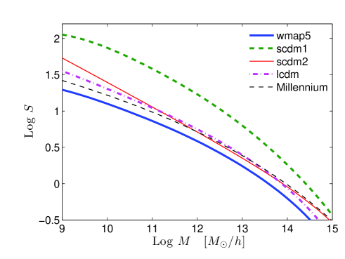
According to the Extended Press-Schechter formalism the statistical properties of merger trees are fixed by the density field at early times when perturbations grow linearly. All the statistical properties of this field are described by its variance, $S(M)=\sigma^{2}(M)$. Specifically, $S(M)$ is the variance of the density field, smoothed with a spherical top hat filter in space, and linearly extrapolated to $\emph{z}=0$ (for more details, see Lacey & Cole, 1993). In fig. 1 we plot $S(M)$ for all the simulations used in this work. This comparison shows the predicted similarity between merger trees of different simulations: we have two simulations with very similar $S(M)$ but different $\Omega_{\rm m}$ (lcdm & scdm2). One simulation has a low value of $\sigma_{8}$ (wmap5), and the scdm1 simulation has a very different shape of $S(M)$.

In order to avoid deviations of $S(M)$ due to the small box size and cosmic variance we measured it directly from the initial condition density field used for each simulation. The values of $\sigma_{8}$ given in table 1 are those obtained by this calibration method. For the scale free simulation (scdm2) the box size is important as it limits contributions from large scales to the field variance (see a detailed discussion in Smith et al., 2003). This effect bends $S(M)$ slightly at the high mass end, in agreement with the theoretical prediction.

3 Conditional Mass Function

This section is devoted to a comparison of the conditional mass function (CMF) as extracted from our suite of $N$-body simulations. The scaling laws of the CMF are important as they highly constrain the behaviour of the full statistics of merger trees. In Appendix A we show other statistical properties of trees, and demonstrate that they follow approximately the properties of the CMF found here.

According to the Extended Press-Schechter formalism (EPS, Bond et al., 1991; Bower, 1991; Lacey & Cole, 1993), the average number of progenitors in the mass interval $[M,M+{\rm d}M]$, which will merge into a descendant halo $M_{0}$ after a timestep $\Delta\omega$, is given by

$$\frac{{{\rm d}}N}{{{\rm d}}M}(M|M_{0},\Delta\omega){\rm d}M\,\;={M_{0}\over M}f(\Delta S,\Delta\omega)\left|\frac{{\rm d}S}{{\rm d}M}\right|{\rm d}M\;\,.$$ (1)

Here $\omega\equiv\delta_{c}(\emph{z})/D(\emph{z})$, where $\delta_{c}(\emph{z})\simeq 1.68$ with a weak dependence on z, and $D(\emph{z})$ is the cosmological linear growth rate. $\Delta\omega\equiv\omega-\omega_{0}$ where the progenitors are identified at $\omega(\emph{z})$ and the descendant halo at $\omega_{0}$. We refer the reader to the appendix of ND08a for a detailed summary on how to compute $\omega$, and a simple fitting function. The quantity $f\,{\rm d}S$ describes the fraction of mass of the descendant halo that is in progenitors of mass in the range $[S,S+{\rm d}S]$. According to EPS

$$f_{\rm ps}(\Delta S,\Delta\omega)=\frac{1}{\sqrt{2\pi}}\;{\Delta\omega\over(\Delta S)^{3/2}}\;{\rm exp}\left[-{(\Delta\omega)^{2}\over 2\Delta S}\right]\,,$$ (2)

where $\Delta S\equiv S(M)-S(M_{0})$, and $f_{\rm ps}$ is the specific solution of $f$ given by the EPS formalism. In what follows we will use the name ‘CMF’ to designate ${\rm d}N/{\rm d}M$ only.

In the language of the EPS formalism $f_{\rm ps}$ is ‘universal’ – it does not explicitly depend on the descendant halo mass $M_{0}$ or on the background cosmology. These parameters appear only in the transformation of $\Delta S$ and $\Delta\omega$ to mass and time (or redshift). The limited success of the EPS formalism in reproducing the $N$-body simulation merger trees indicates that the function $f_{\rm ps}$ is a limited approximation, but it is possible in principle that $f_{\rm ps}$ has universal properties. Both Sheth & Tormen (2002) and Cole et al. (2008) found that $f$ as derived from $N$-body simulations shows non-negligible deviations from universality. However, these studies did not explore in detail the breakdown of universality and did not test other models for $f$ against $N$-body simulations. For example, Cole et al. (2008) have studied $f$ only for descendant haloes identified at $\emph{z}=0$ and showed deviations of $\sim 50\%$ for various values of $\Delta\omega$ and halo masses.

The universality of $f_{\rm ps}$ is based on the two main theoretical elements of the EPS formalism, namely the dynamics of the spherical collapse model and the statistical properties of the initial density fluctuation field when smoothed with a top-hat filter in $k$-space. Variants of these elements have been attempted, including ellipsoidal collapse or smoothing filters of different shapes (Bond et al., 1991; Sheth & Tormen, 2002; Zentner, 2007; Desjacques, 2008). In these models $f$ may in principle depend on the descendant halo mass and thus become non-universal, but this is not necessarily so. For example, Moreno et al. (2008) showed that when ellipsoidal collapse is assumed, $f$ remains universal if the variables $S(M)$ and $\Delta\omega$ are normalized by $S(M_{0})$ and $\sqrt{S(M_{0})}$ respectively. In its most general form, $f$ may depend on $S_{0}\equiv S(M_{0})$, $\omega_{0}$ and the specific cosmology used. We will show below that neglecting the dependence on $\omega_{0}$ and on cosmology may not be too harmful, but the dependence on $S_{0}$ must be properly taken into account for an accurate description of the CMF.

3.1 Self-similarity in time

According to eq. 1, the CMF as predicted by EPS depends only on $\Delta\omega$ and not on the redshift $\emph{z}_{0}$ where the descendant halo is defined. This self-similarity implies that merger trees extracted at different redshifts are self-similar when using $\omega$ as the time variable. Indeed, ND08a and Genel et al. (2008) have verified this behaviour using merger trees extracted from the large Millennium simulation (Springel et al., 2005). It was shown to work well for main-progenitor histories and merger rates, with scatter of a few percent up to $\emph{z}\sim 5$ (see also Fakhouri & Ma, 2008, who found deviations from this symmetry using a different definition of the halo mass).

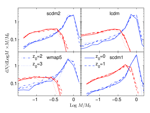
In fig. 2 we show the level of self-similarity in time in our four $N$-body simulations. The scdm1 and scdm2 simulations show small variations in the CMF between different values of $\emph{z}_{0}$, consistent with the sampling noise. The wmap5 and lcdm cosmologies show larger deviations, up to a factor of two for small progenitors and for the time-step $\Delta\omega=0.5$. However, the data do not show a monotonic trend with $\emph{z}_{0}$, hinting that our small-number statistics may contribute to the scatter. For example, the number of descendant haloes within a mass range $10^{12}\leq M_{0}\leq 10^{13}\,\,h^{-1}{M_{\odot}}$ in the wmap5 cosmology is roughly (500,400,100,100) for $\emph{z}_{0}=(0,1,2,3)$ respectively. It is encouraging that better results were obtained for the Millennium simulation (as described above) and for large time-steps. Nonetheless, part of the deviation from self-symmetry may be related to the way haloes are defined using fof linking length and the variation with redshift implied by this definition. As explained in section 2, we try to correct the merger trees for ’backsplash’ haloes. This correction may introduce some additional asymmetry between $\emph{z}_{0}=0$ and higher redshifts.

Figure 2: Self-similarity in time of the progenitor conditional mass function (CMF). Each panel shows the CMF as measured from a different $N$-body simulation as indicated. The descendant halo is identified at different times corresponding to redshifts $\emph{z}_{0}=0,1,2,3$ (solid, dashed, dotted-dashed, and dotted lines respectively). The progenitors are identified at two lookback times corresponding to $\Delta\omega=0.5,3$ (blue and red lines respectively). The distribution of descendant masses is selected in the range $10^{12}\leq M_{0}\leq 10^{13}\,\,h^{-1}{M_{\odot}}$ such that it produces the same distribution of $M_{0}$ in the different cases of $\emph{z}_{0}$. In each case, the four curves show only a weak dependence on the descendant time $\emph{z}_{0}$.

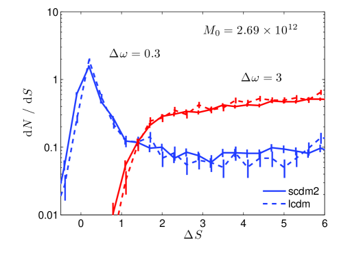
The fact that merger trees remain similar when the descendant time is varied from $\emph{z}=0$ to $\emph{z}=3$ is a non-trivial result. The different values of the cosmological parameters $\Omega_{\rm m}$ and $\Omega_{\Lambda}$ at high redshift imply that the merger trees for a higher $\emph{z}_{0}$ evolve in a different cosmological background. Thus, the dependence of merger trees on the cosmological parameters $\Omega_{\rm m}$ and $\Omega_{\Lambda}$ should be all folded into the time variable $\omega=\delta_{c}/D$. In fig. 3 we test this hypothesis explicitly by comparing the CMF from the scdm2 and lcdm simulations. These simulations have a similar shape of $S(M)$ (see fig. 1) but very different $\Omega_{\rm m}$ values. The agreement is within the Poisson sampling error-bars, demonstrating that $\omega$ can scale properly different expansion histories of the Universe.

Figure 3: Self-similarity of the CMF with respect to the cosmological expansion history. The two sets of CMF are computed for $\emph{z}_{0}=0$, for descendant mass in the range $10^{12}\leq M_{0}\leq 10^{13}\,\,h^{-1}{M_{\odot}}$, and for $\Delta\omega=0.3,3$ (blue and red lines respectively). The solid and dashed lines refer to the scdm2 and lcdm simulations respectively. The distribution of descendant masses at $\emph{z}_{0}$ is matched in order to produce the same distribution of $S(M_{0})$ values, and the average descendant halo mass is indicated in units of $\,h^{-1}{M_{\odot}}$. Note that we plot the number of progenitors per unit of $S$, which is given by eq. 1 times $|{\rm d}M/{\rm d}S|$. The CMF shows only a weak dependence on cosmology.

3.2 Different power-spectrum

Following the EPS formalism (eq. 2) the fraction of mass inside progenitors, $f_{\rm ps}(\Delta S,\Delta\omega)$, depends only on $\Delta\omega$ and $\Delta S$. As mentioned above, one could assume less universal form, $f(\Delta S,\Delta\omega|S_{0})$ that will enable accurate description of the CMF for various cosmological models. In order to test this we plot $f$ in fig. 4 for two sets of power-spectra. The results of the first comparison (left panels) between lcdm and wmap5 simulations is very good, showing no significant deviation in $f$ between these models. This is obtained when the same values of $M_{0}$ are selected in each cosmology, or the same $S_{0}=S(M_{0})$. The difference between these two selection criteria is negligible, so we actually sample $f(\Delta S,\Delta\omega|S_{0})$ for a small range in $S_{0}$.

The second comparison (right panels) shown in fig. 4 is for wmap5 and scdm1 cosmologies. As seen in fig. 1 both $S(M)$ and its derivative ${\rm d}S/{\rm d}M$ vary significantly between these two simulations. This is being translated into a large discrepancy in $f$ when the same values of $M_{0}$ are chosen from both simulations. However, selecting a sample with the same $S_{0}$ values leaves $f$ invariant, proving that $f=f(\Delta S,\Delta\omega|S_{0})$ (at least for our limited set of data). For a given $S_{0}$ the values of $M_{0}$ in both simulations differ by a factor of $\sim$10, limiting the dynamical range for which we can check this $f$ scaling.

Figure 4: Fraction of mass in progenitors for different power spectra and cosmologies. The lines of two types in each panel compare results from two different simulations as indicated. The time steps are $\Delta\omega=0.3,2$ and the descendant haloes are selected at $\emph{z}_{0}=0$. In the left and right panels the descendant halo masses in wmap5 were selected in the range $10^{13}\leq M_{0}\leq 10^{14}\,\,h^{-1}{M_{\odot}}$ and $10^{12}\leq M_{0}\leq 10^{13}\,\,h^{-1}{M_{\odot}}$ respectively. In lcdm and scdm1 the descendant haloes were chosen to match the distribution of $M_{0}$ or $S_{0}$ in wmap5, as indicated in each panel.

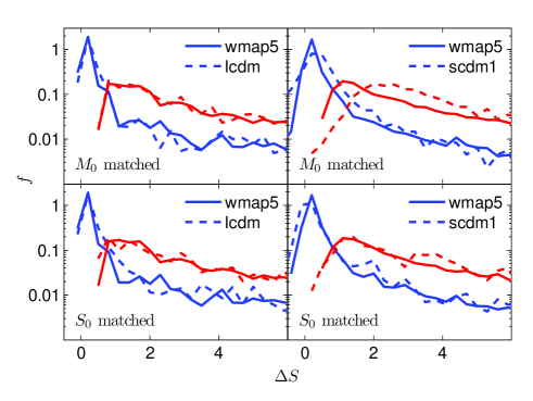
The dependence of $f$ on $S_{0}$ deserves a more careful test, probably with a larger set of $N$-body simulations, spanning a larger range of power-spectra. It is important to verify that such a dependence is not related to the shape of $S(M)$, as was found here. If this is true, it implies that a modification to the normalization of the power-spectrum ($\sigma_{8}$) which changes $S_{0}$, will induce a non-trivial change to the CMF. Such a dependence on $\sigma_{8}$ is different from the simple scaling of the shape $\Delta\omega/\sqrt{\Delta S}$ that is used by EPS (see below).

3.3 Global fitting function

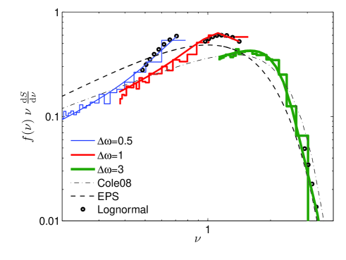
The EPS formalism suggests that the mass ($\Delta S$) and time ($\Delta\omega$) variables can be scaled into a new variable $\nu\equiv\Delta\omega/\sqrt{\Delta S}$. In terms of $\nu$, the function $f(\nu)\,\nu\,{\rm d}S/{\rm d}\nu$ should be universal. As shown above some dependence on $S_{0}$ is required, so we can try to use a function of the shape $f(\nu|S_{0})$. This is tested in fig. 5 where we plot $f(\nu|S_{0})$ for a fixed value of $S_{0}$ and for various $\Delta\omega$. The clear deviations from a unique line show that such a formulation is too simple and incompatible with the results of $N$-body simulations. This figure is very similar to the one given in Sheth & Tormen (2002) and Cole et al. (2008), and agrees with these previous results. Thus, we are forced to use a more general form $f=f(\Delta S,\Delta\omega|S_{0})$.

Figure 5: The limitation of using a fitting function of the form $f(\nu|S_{0})$. The results form the scdm2 simulation are plotted as histograms. They are extracted at $\emph{z}_{0}=0$ with three different time steps $\Delta\omega=0.5,\,1,\,3$ and for an average halo mass of $3\times 10^{12}\,\,h^{-1}{M_{\odot}}$. The global fit of eq. 3.3 for the three time steps is shown as smoothed solid curves. The EPS prediction is plotted as a thin dashed line and the fit of Cole et al. (2008) is shown as a dotted-dashed line. Like any other function of the type $f(\nu)$, they both fail to reproduce the simulation results. The lognormal global fit to $P_{1}$ (eqs. 5 & 6) is plotted as small circles (only for $M>M_{0}/2$, where it should be identical to the CMF, see section 4).

We found that the fitting function below can fit the CMF from our set of $N$-body simulations for all time-steps larger than $\Delta\omega\sim 0.5$ and all $S_{0}$ values. We have looked for the simplest possible function that can fit the data, which is still similar to the EPS original function. The function we adopt is:

$$f(\Delta S,\Delta\omega|S_{0})=a\frac{\Delta\omega}{\Delta S^{1.5}}\exp\left[-b\frac{\Delta\omega^{2}}{\Delta S}\right]+$$

$$c\frac{\Delta\omega^{2}}{\Delta S^{3}}\exp\left[-d\frac{\Delta\omega^{2.5}}{\Delta S^{2+\alpha}}\right]\,,$$

where the parameters explicitly depend on $S_{0}$ in the following way:

$$a = 0.215+0.0037\,S_{0}$$

$$b = 0.414+0.0013\,S_{0}^{2}$$

$$c = 0.0746+0.0382\,S_{0}$$ (4)

$$d = 0.257+0.0568\,S_{0}$$

$$\alpha = -0.0141\,S_{0}+0.0056\,S_{0}^{2}$$

The added term is not a natural feature of the standard EPS formalism, and it emphasizes the need for additional physics, beyond the Sheth-Tormen generalization from spherical to ellipsoidal collapse model. The failure of functions that depend solely on $\nu$ in reproducing the detailed evolution of $N$-body simulations may have interesting theoretical implications. We also note that our fitting function is not necessarily unique — there may exist other fitting functions of comparable quality. However, it is likely to be sufficient for most applications related to galaxy formation, based on the tests performed here over wide ranges of halo masses, redshifts and cosmological models.

Figure 6: A global fit to $f(\Delta S,\Delta\omega|S_{0})$ as defined in eqs. 3.3 and 3.3. Each panel refers to a given set of $S_{0}$ and $\Delta\omega$ values as indicated. The simulation data (histograms) were extracted and averaged from all the different simulations used here at $\emph{z}_{0}=0$ and at $\emph{z}_{0}=1$. The descendant masses were selected in log bins of size half dex. Our global fit, the EPS prediction, the fit of Cole et al. (2008), and the fit of Sheth & Tormen (2002) are shown as solid, dashed, dashed-dotted and dotted lines respectively. Note that both the EPS prediction and the fit of Cole et al. (2008) are independent of $S_{0}$.

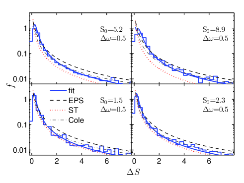
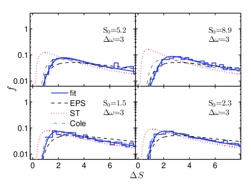
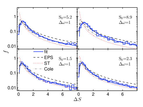
In fig. 6 we compare our fitting function to the simulation data, showing that it accurately reproduces the trends found. The agreement between the fit and data is at the level of the statistical noise. The dependence on $S_{0}$ is mainly seen at low $\Delta S$ (corresponding to massive progenitors). We also show the EPS prediction and the fit derived by Cole et al. (2008), both independent on $S_{0}$. Evidently, our fit agrees well with Cole et al. (2008) for intermediate and massive haloes (although deviations for massive progenitors are highlighted in fig. 5). This is encouraging because the fits are based on different simulations and different merger-tree construction schemes. However, our fit breaks the symmetry of using only $\nu$ as was done by Cole et al. (2008), in this way it can capture the behaviour of the data for low mass haloes, and across various time-steps. The accuracy for different $\Delta\omega$ can be specifically seen in fig. 5.

The integral of $f$ can be computed analytically only for $\alpha=2$ ($S_{0}\sim 2.5$), for the whole halo mass range we computed the integral numerically, yielding 0.75 up to 0.9, depending on the descendant mass and on the time-step. This predicts that a substantial fraction of the mass is not included in any progenitors but rather accreted from a ‘smooth’ component.

Throughout this work we mainly discuss the EPS formalism in its standard version. However, as mentioned in the introduction, versions of this formalism which use the ellipsoidal collapse model are presumably more accurate, as is indicated by their ability to predict accurate halo mass functions. We examine two such studies, the pioneer work of Sheth & Tormen (2002) and a more recent work by Moreno et al. (2008). Our interpretation of both studies is that the CMF as predicted by the spherical model is comparable in its accuracy to the one predicted by ellipsoidal collapse. This can be seen in figs. 7 & 8 of Sheth & Tormen (2002). More evidently, figs. 3-5 of Moreno et al. (2008) show that the spherical model gives better results for low mass descendant haloes, but this trend changes for massive haloes, where the ellipsoidal collapse is more accurate. We also show in fig. 6 the CMF proposed by Sheth & Tormen (2002) . It is clear that this model predicts CMFs which are significantly higher from the simulation results in the regime of massive progenitors and large time-steps. Note that plotting $f(\Delta S,\Delta\omega|S_{0})$ shows more clearly this effect than the usual plot as a function of mass ratio (e.g. Moreno et al., 2008). In Appendix A.3 we provide more results in the form of fig. 6

4 Main-Progenitor Histories

The “main-progenitor” history of a given merger-tree is constructed by following backward in time the most massive progenitor in each merger event. This is a useful definition as it allows us to follow a well defined branch of the tree. In addition, a quantitative description of the main-progenitor history highly constrains the full statistics of trees. Properties of main-progenitor histories were studied extensively, both analytically and using $N$-body simulations (Lacey & Cole, 1993; Nusser & Sheth, 1999; Firmani & Avila-Reese, 2000; Wechsler et al., 2002; van den Bosch, 2002; Neistein et al., 2006; Li et al., 2007; Neistein & Dekel, 2008a; Zhao et al., 2008). Let us also mention that the main-progenitor is not always the most massive progenitor at a given time.

We define $P_{1}$ as the probability density to find a main-progenitor of mass $S(M_{1})$ for a given descendant halo mass $M_{0}$, and a time-step $\Delta\omega$. As was found by ND08a, $P_{1}$ can be well fitted by a lognormal distribution,

$$P_{1}(\Delta S_{1}|S_{0},\Delta\omega)=\frac{1}{\sigma_{p}\Delta S_{1}\sqrt{2\pi}}\exp\left[-\frac{(\ln\Delta S_{1}-\mu_{p})^{2}}{2\sigma_{p}^{2}}\right]\,.$$ (5)

Here $\Delta S_{1}=S(M_{1})-S(M_{0})$, the parameters $(\sigma_{p},\mu_{p})$ depend on $S_{0}$ and $\Delta\omega$, and as usual $S_{0}\equiv S(M_{0})$. By definition, the integral over $P_{1}(\Delta S_{1})$ equals unity for any $S_{0}$ and $\Delta\omega$.

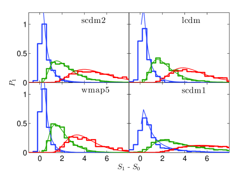
Main-progenitor histories were constructed for all the simulations used in this work. Following ND08a, we confirm that the lognormal distribution fits accurately the simulation results. This was tested for all possible ranges of halo masses, redshift, and time-steps. As was mentioned by ND08a the fit becomes inaccurate for small time steps, typically for $\Delta\omega\lesssim 0.5$. Such a behaviour is found here as well. One exception to the above, where the lognormal fit is somewhat innacurate, is for the scdm1 simulation at $\emph{z}_{0}=0$. This may be due to the high sensitivity of $\Delta S$ in this cosmological model (${\rm d}S/{\rm d}M$ is typically 7 times larger than other cases). The fact that the fit works well for $\emph{z}\gtrsim 1$ data using the same cosmological simulation is encouraging. In fig. 7 we plot main-progenitor distributions for few cases of halo mass, $\emph{z}_{0}$ and $\Delta\omega$, more examples can be found in Appendix B. The accuracy of the lognormal fit as plotted here is typical for the rest of the cases.

Figure 7: The distribution of main progenitor masses in different cosmological models. Results are shown for descendant haloes defined at $\emph{z}_{0}=1$ and for main progenitors at two different time steps, $\Delta\omega=0.5,\,3$. The descendant halo mass is in the range $10^{12}\leq M_{0}\leq 4\times 10^{12}\,\,h^{-1}{M_{\odot}}$ for the wmap5 cosmology, and $M_{0}$ in the other cosmologies were selected to match the same distribution of $S(M_{0})$. Thin solid lines show the lognormal global fit, eq. 6, as computed for the lcdm and scdm1 cases.

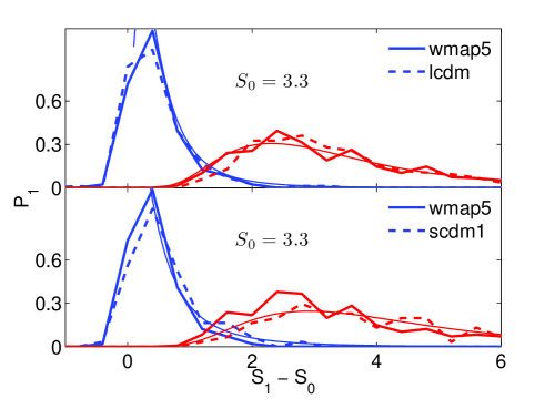
For each cosmology we are able to use a global fit, similar to the one suggested by ND08a. The fit approximates the standard deviation and average of $\ln\Delta S_{1}$ by

$$\sigma_{p} = (a_{1}\log S_{0}+a_{2})\log\Delta\omega+a_{3}\log S_{0}+a_{4}$$ (6)

$$\mu_{p} = (b_{1}\log S_{0}+b_{2})\log\Delta\omega+b_{3}\log S_{0}+b_{4}\,.$$

We provide numerical details for the values of these parameters in Appendix B. For a given $S_{0}$, the evolution with time of $\sigma_{p}$ and $\mu_{p}$ is simply linear in $\log\Delta\omega$. In fig. 5 we show that this evolution gives a very accurate fit to the relevant part of the CMF (the CMF and main-progenitor distribution are identical for $M>M_{0}/2$). We recall that such time-evolution was obtained for the CMF using much more complicated $\Delta\omega$ dependence (see eq. 3.3). Although both approaches discuss only the fitting possibilities, it seems that the main-progenitor gives a much simpler way to describe the merger history in an accurate way.

The simple behaviour of $P_{1}$ for each cosmology as seen in eq. 6 and in fig. 5 calls for a more global fit, which predicts the parameters of $P_{1}$ in other cosmological models. We compared $P_{1}$ for our set of simulations and found a high level of self-similarity, with the exception of the scdm1 case. Unfortunately we could not find a general law able to combine scdm1 with the other cosmological models. For example, choosing haloes with the same values of $S_{0}$ from scdm1 and other simulations does not yield the same results. To summarize, our study indicates that the main-progenitor distribution as extracted from $N$-body simulations has a universal lognormal shape. However, the dependence of the lognormal parameters on cosmology is not clear, and there is no theoretical explanation to this phenomena yet.

Recently, Zhao et al. (2008) studied the behaviour of main-progenitor histories for different cosmological models. They provide a fitting procedure for estimating median main-progenitor histories in any cosmological model. However, we find it hard to estimate the full distribution $P_{1}(\Delta S)$ out of their algorithm.

5 Applications

An accurate fitting function for the CMF includes substantial information on halo growth, and it has various interesting applications: it can shed more light on the evolution of the halo mass function with redshift and cosmology (e.g. Tinker et al., 2008), it can constrain dark energy models, it is useful for generating Monte-Carlo merger trees, and for predicting mass-accretion histories of the main-progenitor. Here we focus on a new methodology for re-scaling a given set of merger trees between different cosmological models. We also discuss briefly the possibility of generating Monte-Carlo trees.

Figure 8: The conditional mass function (CMF), ${\rm d}N/{\rm d}M$, computed for different cosmological models using a transformation of the time-step $\Delta\omega$. In each panel we compare results from two different simulations and for the same descendant halo mass as indicated (in units of $\,h^{-1}{M_{\odot}}$). The time steps used for the lcdm cosmology are $\Delta\omega=0.5,\,2$. For the wmap5 and scdm1 simulations they are different by a factor of 0.86 and 1.8 respectively. We learn that the time transformation allows a reasonable scaling of the merger trees, albeit with certain deviations in some cases.

5.1 Re-scaling a given merger tree

There are many existing resources of $N$-body simulations and related merger trees which are publicly available. The most useful one being the Millennium simulation (Springel et al., 2005) with its web-based database (Lemson et al., 2006). However, recent changes in the observed values of cosmological parameters (especially $\sigma_{8}$) make these simulations inaccurate for predicting observable quantities in our Universe. Here we suggest a new methodology to transform merger trees into a different cosmological model, halo mass, and redshift. Such transformation can also be useful for enhancing the mass resolution of merger trees. There are few benefits for this approach over the standard method of generating Monte-Carlo trees: (a) it can preserve the non-Markov behaviour of trees (see e.g. ND08a) (b) it might be easily extended to handle substructures (c) it might be extended to accurate transformation of halo spatial locations.

We define the case $r$ as our reference data from a given merger-tree,

$$\{M_{i}\,|M_{0},\Delta\omega,C\}_{r}\,$$ (7)

The data is defined as a set of progenitors $M_{i}$ for a given descendant halo mass $M_{0}$, time-step $\Delta\omega$ and a cosmological model $C$. Our target case is defined as a different cosmology $\widetilde{C}$ and descendant mass $\widetilde{M}_{0}$

$$\{\widetilde{M}_{i}\,|\widetilde{M}_{0},\widetilde{\Delta\omega},\widetilde{C}\}_{t}\ .$$ (8)

We are looking for a transformation of the kind

$$M_{i}\rightarrow\widetilde{M}_{i}\;\;\;\;,\;\;\;\;\Delta\omega\rightarrow\widetilde{\Delta\omega}$$ (9)

that will yield a different set of progenitors, possibly for a different time-step, which will be consistent with the target case. Such a consistency is achieved when the transformed progenitors will yield the proper CMF. Note that our global fit was done for $f(\Delta S,\Delta\omega|S_{0})$, as seen from eq. 1 the CMF includes two other components, the mass ratio $M_{0}/M$ and the derivative ${\rm d}S/{\rm d}M$. As a result, transformations that will yield the appropriate CMF cannot be done using the information imprinted in $f$ alone, and the functional dependence of $S$ on $M$ should be important.

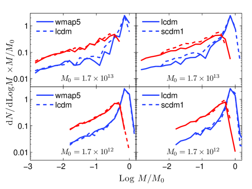
We start by searching for the most accurate transformation in $\Delta\omega$ which can compensate for the change in cosmology $C$, or descendant halo mass $M_{0}$. This means that we only change $\Delta\omega$ into $\widetilde{\Delta\omega}$ while keeping the masses of the descendant and progenitor haloes fixed. In the general case, such a simple transformation might not allow us to accurately transform the trees. In practice, it might be a good starting point for many relevant cases. Our methodology to find time-transformation is as follows: for a given reference case we use eq. 3.3 to compute the reference CMF. We then compute the CMF for the target case using various time-steps $\widetilde{\Delta\omega}_{i}$. The value of $\widetilde{\Delta\omega}$ is chosen from the set of $\widetilde{\Delta\omega}_{i}$ in order to give the best match between the reference and the target CMF’s.

In fig. 8 we plot the CMF for two sets of cosmologies where time transformation is being used. This transformation is relatively accurate, although it can introduce a large transformation in time (almost a factor of 2 in $\Delta\omega$ for one of the cases tested here). The original differences between the simulations can be seen in fig. 2 for reference. Nonetheless, it seems that the transformation in $\Delta\omega$ do not provide a uniform accuracy for all descendant masses. In fig. 9 we show how changing $\Delta\omega$ can compensate for different descendant halo masses. This indicates that enhancement of mass resolution can be easily obtained.

Time transformations are limited in accuracy, and can lower the time resolution of a merger-tree significantly. In addition, such transformations might stretch the non-markov correlations between consecutive time-steps in a way that might be different from the behaviour of the simulations. Our statistical sample does not allow us to explore the last effect in detail.

Figure 9: The conditional mass function (CMF) for different descendant halo masses and at at different time-steps as indicated. The figure demonstrates that the transformation $\widetilde{\Delta\omega}=1.3\times\Delta\omega$ properly compensates for the change in descendant mass $M_{0}$.

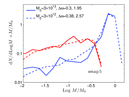
A less trivial transformation is needed when the time scaling cannot provide an accurate enough solution. In this case we can transform the mass of the progenitor haloes in order to yield the same CMF. For any progenitor mass $M$ we define $\widetilde{M}$ such that the integral over the number of progenitors will be invariant,

$$\widetilde{M}:\;\;\;\int_{\widetilde{M}}^{\widetilde{M}_{0}}\left[\frac{{\rm d}N}{{\rm d}M}\right]_{t}{\rm d}M=\int_{M}^{M_{0}}\left[\frac{{\rm d}N}{{\rm d}M}\right]_{r}{\rm d}M\,.$$ (10)

This equation can be used to find the transformation $M\rightarrow\widetilde{M}$ numerically using the global fitting function of eq. 3.3. In fig. 10 we show that this transformation can yield perfect matching between very different CMF’s. The only limitation in the accuracy is the goodness of our global fit, which is used to find the mass transformation above. As shown in fig. 10 the same mass transformation is suitable for a large range of time-steps, so the deviations of the CMF fit at small time-steps do not degrade the accuracy of the mass transformation.

Figure 10: Scaling the mass in order to compensate for the change in ${\rm d}N/{\rm d}M$. We use eq. 10 to transform the mass of progenitors from the wmap5 simulation (solid blue lines) into the scdm1 model (dashed red), both at the same time $\Delta\omega$. The mass transformation $M_{i}\rightarrow\widetilde{M}_{i}$ derives from the global fit at a specific time-step, $\Delta\omega=1$. The same transformation is used to transform the actual progenitor masses for all the time steps used here. The dashed-dotted lines show the resulting CMF values, which are similar to the target case. The descendant halo mass is $10^{12}\,\,h^{-1}{M_{\odot}}$.

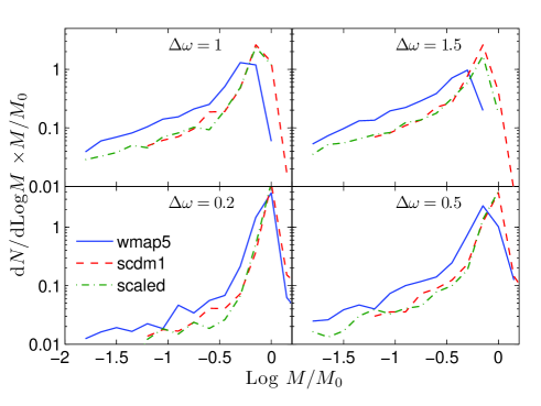
In general, one might use transformation of $\Delta\omega$ and mass according to the specific case needed. Time transformation are much more easy to perform, and should be preferred for cases where the resulting time resolution is not problematic. Mass transformation can be done as a second step, to increase the accuracy of the statistics by small variations in mass. For example, as tested above, using the results of the Millennium simulation (Springel et al., 2005) with a transformation $\widetilde{\Delta\omega}=0.86\Delta\omega$ should give merger trees which are consistent with the cosmological model WMAP5 for a large range of halo masses. For this simple case, the time transformation is consistent with the naive EPS prediction and scales like $\sigma_{8}$.

5.2 Generating Monte-Carlo trees

Constructing Monte-Carlo merger trees is doable once an accurate knowledge of the CMF is given for all time-steps. There are various algorithms that were applied to the EPS CMF, and can be easily generalized for other CMF’s (Kauffmann & White, 1993; Neistein & Dekel, 2008b; Zhang et al., 2008). In this sense our fitting function for the CMF might be very useful for constructing Monte-Carlo trees that fit the results of $N$-body simulations. However, there are some limitations to this approach which we will emphasize here below.

As stated in the previous section, the quality of our global fit is poor for small time steps ($\Delta\omega<0.5$). On the other hand, the time-step which is convenient for constructing Monte-Carlo trees is much smaller, around $\Delta\omega=0.1$. Larger time-steps yield many progenitors in each merger event, and a large uncertainty in the predicted merging time of the haloes. As a result, we do not have an accurate fitting function for the CMF, which is appropriate for generating Monte-Carlo trees. More than that, an accurate fit for the CMF at small $\Delta\omega$ will not provide a solution, because the behaviour of merger trees is highly non-markov at such small time-steps. This means that applying the CMF in consecutive time-steps without proper correlation between steps will generate large deviations in the merger histories (ND08a).

A possible solution to these problems is to look for a new CMF at small time-steps that will reproduce the CMF from $N$-body simulations at big time-steps. The CMF at small $\Delta\omega$ does not have to match $N$-body simulations, it can only be tested by applying it on few consecutive time-steps. Such a methodology was introduced by ND08a and found to produce good results. However, the resulting trees are fully markov, differing from $N$-body simulations. As a result of the above complications we think that this problem deserve more room than what is left here, and we postpone it to a future work.

6 Summary and Discussion

We provide an improved description of the merger histories of dark-matter haloes as measured from $N$-body simulations. Using a suite of cosmological simulations, and a range of descendant halo masses at different redshifts, we provide a robust fitting function for the conditional mass function of progenitors, the CMF. This fit emphasizes the self-similar and universal nature of the merger trees and it is more accurate than earlier attempts (Lacey & Cole, 1993; Sheth & Tormen, 2002; Moreno et al., 2008; Cole et al., 2008). The improved fit is owing to the functional form used, which generalizes the EPS formula with a term that breaks the symmetry between the natural time and mass variables. An improved accuracy is achieved by allowing the best-fit parameters to explicitly depend on the descendant halo mass. We note that it might be that other fitting functions will describe the data in a similar accuracy, and that our formula will deviate from the simulation results at different halo mass ranges. However, the range in halo mass probed in this work dominates the contribution to galaxy formation processes.

The accurate fitting function for the CMF can serve as a basis for comparing different simulations, or different algorithms for construction merger trees. It can also be used for testing new modifications to the theory (e.g. Maggiore & Riotto, 2009) and for constraining the time evolution of the halo mass function (Tinker et al., 2008). We discuss a specific application of our fitting function, that is to scale merger trees that are extracted from a given $N$-body simulation into a different cosmological model, or different ranges of mass or redshift. We demonstrate that these scalings provide more accurate merger trees than other methods that utilize Monte-Carlo realizations. The scaling method conserves the correlation of the progenitor masses between time-steps, a non-Markovian effect that is hard to mimic in Monte-Carlo generated trees. It would be worthwhile to study the scaling of substructures along similar lines. Substructures should be affected mostly by the mass ratio of the subhalo to its host halo, and by the dynamical time-scale within the host. Once these quantities are conserved, substructures might be easily scaled as well. Such an analysis of substructures requires simulations of higher resolution than those used here.

While most predictions of the EPS approximation are inaccurate, we find that the self-similarity in time proposed by EPS is valid to an accuracy of a few percents. We show explictly that merger histories are self-similar when using the time variable $\omega=\delta_{c}/D(t)$, with $\delta_{c}\simeq 1.68$ and $D(t)$ the cosmological linear growth rate. This self-similarity, which has been noticed by Neistein & Dekel (2008a) and Genel et al. (2008) in the Millennium simulation (Springel et al., 2005), is verified here for different cosmological models. We show that this self-similarity implies that $\omega$ can be used for relating merger trees from different cosmologies.

In this work we used as default a standard halo definition based the fof algorithm with a linking length corresponding to 20% of the mean interparticle separation. We tested in comparison merger trees for haloes defined using a spherical overdensity (SO) method (for more details on how these trees are defined see Macciò et al., 2008), and found that they are less self-similar in time, and are thus not as suitable for obtaining a universal fitting function. Indeed, the fof haloes are known to provide a better match to the theory (Lacey & Cole, 1994), and they are therefore more commonly used in the relevant literature (e.g. Sheth & Tormen 2002, Cole et al., 2008).

The construction of a merger tree by linking haloes from different simulation snapshots can be done in different ways, and the results may depend on the method adopted. A comparison of our results and other results from the literature indicates that this is not an issue of major concern. For example, Cole et al. (2008) does not report a noticable difference between their CMF results and those of Bower et al. (2006), which use different algorithms for constructing merger trees. On the other hand, our progenitor definition is very similar to the one used by Sheth & Tormen (2002), so the improvement in the fitting quality is not likely to be due to deviations in the simulation results. Finally, merger trees that were constructed by different methods may differ at small time steps, but these differences tend to diminish when large time steps are considered, e.g. the $\Delta z>0.5$ steps used in our analysis (see e.g. Genel et al., 2008, and their figure 8b).

Our current analysis of a suite of cosmological simulations confirms the lognormal nature of the main-progenitor distribution as a function of the natural mass variable $\sigma^{2}(M)$, as reported by Neistein & Dekel (2008a) from the Millenium simulation. The linear dependence of the parameters of the lognormal distribution on the natural time variable $\log\Delta\omega$ is much simpler than the time dependence of the CMF fit described in the first part of our paper. This motivates a theoretical search for the origin of the lognormal distribution of main progenitors. Both methods used here to quantify merger-trees as measured from $N$-body simulations emphasize the limits of current theories in capturing the details of dark-matter evolution.

Appendix A Additional Statistics

A.1 Self-similarity in time

In this section we provide more details on the accuracy of the self-similarity in time, as discussed in section 3.1. In fig. 11 we plot average main-progenitor histories for our set of simulations. The histories are plotted for descendant haloes identified at $\emph{z}_{0}=0,1,2$. Comparing histories for different $\emph{z}_{0}$ we see small deviations with $\emph{z}_{0}$, reaching $\sim 20\%$ at $\Delta\omega=5$ (for the scdm1 & lcdm simulations). It should be kept in mind that cosmic variance is non-negligible in this plot. We also plot the EPS prediction for the main-progenitor histories, as given by Neistein et al. (2006). The difference between the analytical EPS prediction and the results of $N$-body simulations seem to change slightly with halo mass. These results are sometimes different from the study of Zhao et al. (2008). We note that these authors compared median values from simulations against average values from the EPS formalism, as estimated by van den Bosch (2002). This makes their comparison less accurate than what is done here.

Figure 11: Average main-progenitor histories at different times. Smooth lines show main-progenitor histories for descendant halo $M_{0}$ identified at $\emph{z}_{0}=0,\,1,\,2$ ($\emph{z}_{0}=2$ was omitted for the high-mass bin due to a small statistical sample). Symbols and error-bars are the predictions of the EPS formalism following the formula of Neistein et al. (2006), and are independent on $\emph{z}_{0}$. The symbols shapes are diamonds, squares, triangles, circles and pluses for the scdm1, scdm2, lcdm, wmap5, and Millennium simulations respectively. It is evident that self-similarity in time is valid for all the simulations. The deviations of the EPS formalism with respect to $N$-body simulations are similar in all cases, although slight trends with cosmology and halo mass can be seen.

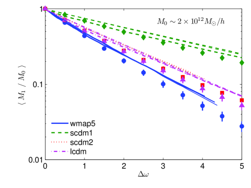
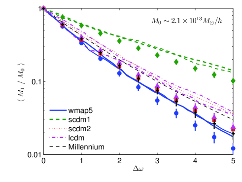
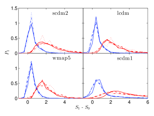
The full distribution of the main-progenitor, $P_{1}(\Delta S|S_{0},\Delta\omega)$, is plotted in fig. 12 for descendant haloes selected at different $\emph{z}_{0}$. Here as well, self-similarity in time is shown to be accurate with the exception of the scdm1 simulation at $\emph{z}_{0}=0$.

Figure 12: The full distribution of the main-progenitor mass at different times. In each panel we plot the results from one simulation as indicated, where the descendant halo mass $M_{0}$ is between $10^{12}$ and $10^{13}\,\,h^{-1}{M_{\odot}}$, and it is selected at $\emph{z}_{0}=0,1,2,3$ (solid, dashed, dashed-dotted, dotted lines respectively). Main-progenitors are followed backwards in time until $\Delta\omega=0.5\,\&\,2$ (blue and red curves respectively).

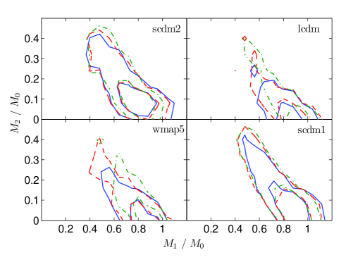
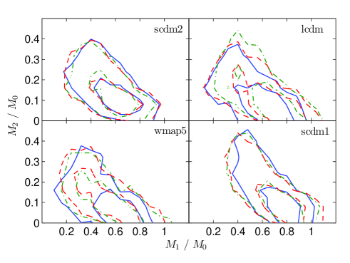
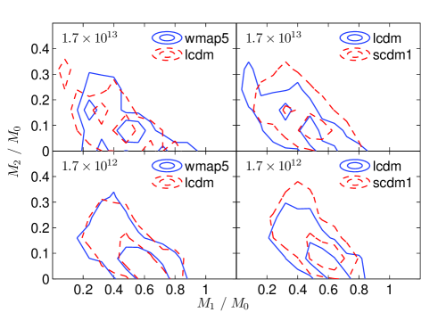
In figs. 13 & 14 we plot the mutual distribution of the two most massive progenitors. We show two dimensional histograms for descendant haloes selected at $\emph{z}_{0}=0,1,2$. The results for scdm1 & scdm2 simulations show accurate similarity for different $\emph{z}_{0}$. However, the lcdm and wmap5 show deviations a the level of 10-20% in mass. These deviations decrease at larger time steps, so they might be connected to non-markov effects at small time-steps, and their variation with redshift. In addition, our treatment of ‘blacksplash’ haloes may affect the results (see the discussion in section 3.1).

Figure 13: The mutual distribution of the two most massive progenitors ($M_{1},\,M_{2}$). Each panel shows results from one simulation as indicated. The descendant halo $M_{0}$ is identified at $\emph{z}_{0}=0,1,2$ (plotted as solid, dashed, dashed-dotted lines respectively). The contour lines are plotted for 7 & 30% of the maximum histogram values. Descendant mass is between $10^{12}$ and $10^{13}$ $\,h^{-1}{M_{\odot}}$, and $\Delta\omega=0.3$ in all cases.

Figure 14: Same as fig. 13 but with $\Delta\omega=0.8$.

A.2 Scaling merger trees

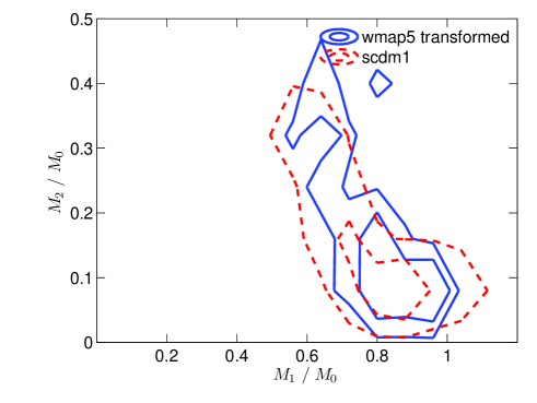
In this section we further examine the scaling of merger trees as it was applied in section A.2. We only show mutual distributions of the two most massive progenitors, $(M_{1},M_{2})$, as the main-progenitor distribution is highly constrained by the CMF (see e.g. Neistein et al., 2006). In fig. 15 we examine the time-transformation which was used to generate fig. 8. The results of the mass scaling as applied in fig. 10 are shown here in fig. 16.

Figure 15: The mutual distribution of the two most massive progenitors ($M_{1},\,M_{2}$), for $\Delta\omega$ matching. The same $\Delta\omega$ transformation is done as in fig. 8. The contour lines are plotted for 13 & 50% of the maximum histogram values. Descendant mass is indicated in units of $\,h^{-1}{M_{\odot}}$, $\Delta\omega=1$.

Figure 16: The mutual distribution of the two most massive progenitors ($M_{1},\,M_{2}$), for mass matching. Mass transformation for wmap5 was done in the same way as in fig. 10. $\Delta\omega=0.3$, $M_{0}=10^{12}\,\,h^{-1}{M_{\odot}}$.

A.3 A global fit to the CMF

In fig. 17 we provide more tests to our global fit, in a similar way to fig. 6.

Figure 17: Similar to fig. 6, but for different time-steps as indicated.

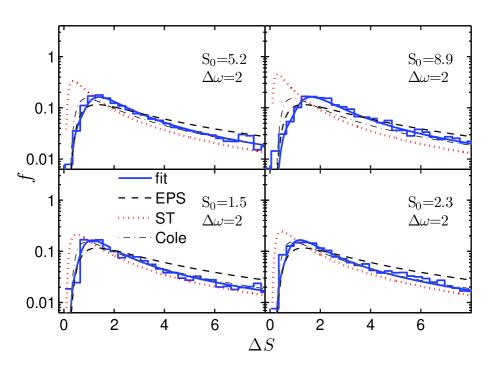
Appendix B A global fit to the main-progenitor distribution

In section 4 we claim that the lognormal distribution can be easily described for all time-steps and descendant masses using eqs. 5 & 6. This is shown in fig. 18, where full distributions of the main-progenitor mass are plotted. In tables 2 & 3 we summarize the parameters of the fits.

Table 2: The coefficients used for the global lognormal fit, eqs. 5 & 6. The standard deviation of $\ln\Delta S$ obeys the equation $\sigma_{p}=(a_{1}\log S_{0}+a_{2})\log\Delta\omega+a_{3}\log S_{0}+a_{4}$, where $a_{i}$ are given below for each cosmology. For the Millennium simulation (MS) we used the fit given by ND08a, and transformed it to depend on $S_{0}$.

Simulation	$a_{1}$	$a_{2}$	$a_{3}$	$a_{4}$
wmap5	-0.333	-0.321	0.0807	0.622
scdm1	-0.0344	-0.608	0.185	0.697
scdm2	0.760	-1.085	0.184	0.668
lcdm	-1.209	0.205	0.245	0.571
MS	0.0135	-0.404	0.102	0.561

Table 3: The coefficients used for the global lognormal fit, eqs. 5 & 6. The mean of $\ln\Delta S$ obeys the equation $\mu_{p}=(b_{1}\log S_{0}+b_{2})\log\Delta\omega+b_{3}\log S_{0}+b_{4}$, where $b_{i}$ are given below for each cosmology. For the Millennium simulation (MS) we used the fit given by ND08a, and transformed it to depend on $S_{0}$.

Simulation	$b_{1}$	$b_{2}$	$b_{3}$	$b_{4}$
wmap5	0.132	2.404	0.585	-0.436
scdm1	-0.8105	3.179	0.988	-0.513
scdm2	0.418	2.366	0.999	-0.647
lcdm	0.0788	2.418	0.671	-0.434
MS	-0.217	2.575	0.662	-0.5627

Figure 18: The full distribution of the main-progenitor for different cosmologies and time-steps. Descendant haloes are selected at $\emph{z}_{0}=1$ with mass between $10^{12}$ and $10^{13}\,\,h^{-1}{M_{\odot}}$. Main-progenitor mass is followed backward in time until $\Delta\omega=0.5,\,2,\,4$. Histograms show the simulation data, smooth lines are generated using our global fit.

References

- Bertschinger (2001) Bertschinger E., 2001, ApJS, 137, 1
- Bond et al. (1991) Bond J. R., Cole S., Efstathiou G., Kaiser N., 1991, ApJ, 379, 440
- Bower (1991) Bower R. G., 1991, MNRAS, 248, 332
- Bower et al. (2006) Bower R. G., Benson A. J., Malbon R., Helly J. C., Frenk C. S., Baugh C. M., Cole S., Lacey C. G., 2006, MNRAS, 370, 645
- Cole et al. (2008) Cole S., Helly J., Frenk C. S., Parkinson H., 2008, MNRAS, 383, 546
- Davis et al. (1985) Davis M., Efstathiou G., Frenk C. S., White S. D. M., 1985, ApJ, 292, 371
- Desjacques (2008) Desjacques V., 2008, MNRAS, 388, 638
- Fakhouri & Ma (2008) Fakhouri O., Ma C.-P., 2008, MNRAS, 386, 577
- Firmani & Avila-Reese (2000) Firmani C., Avila-Reese V., 2000, MNRAS, 315, 457
- Genel et al. (2008) Genel S., Genzel R., Bouché N., Naab T., Sternberg A., 2008, ArXiv e-print 0812.3154
- Jenkins et al. (2001) Jenkins A., Frenk C. S., White S. D. M., Colberg J. M., Cole S., Evrard A. E., Couchman H. M. P., Yoshida N., 2001, MNRAS, 321, 372
- Kauffmann et al. (1999) Kauffmann G., Colberg J. M., Diaferio A., White S. D. M., 1999, MNRAS, 303, 188
- Kauffmann & White (1993) Kauffmann G., White S. D. M., 1993, MNRAS, 261, 921
- Knebe et al. (2008) Knebe A., Arnold B., Power C., Gibson B. K., 2008, MNRAS, 386, 1029
- Komatsu et al. (2009) Komatsu E., et al., 2009, ApJS, 180, 330
- Lacey & Cole (1993) Lacey C., Cole S., 1993, MNRAS, 262, 627
- Lacey & Cole (1994) Lacey C., Cole S., 1994, MNRAS, 271, 676
- Lemson et al. (2006) Lemson G., et al., 2006, ArXiv Astrophysics e-prints, astro-ph/0608019
- Li et al. (2007) Li Y., Mo H. J., van den Bosch F. C., Lin W. P., 2007, MNRAS, 379, 689
- Macciò et al. (2008) Macciò A. V., Dutton A. A., van den Bosch F. C., 2008, MNRAS, 391, 1940
- Maggiore & Riotto (2009) Maggiore M., Riotto A., 2009, ArXiv e-prints/0903.1250
- Moreno et al. (2008) Moreno J., Giocoli C., Sheth R. K., 2008, MNRAS, 391, 1729
- Neistein & Dekel (2008a) Neistein E., Dekel A., 2008a, MNRAS, 383, 615 (ND08a)
- Neistein & Dekel (2008b) Neistein E., Dekel A., 2008b, MNRAS, 388, 1792
- Neistein et al. (2006) Neistein E., van den Bosch F. C., Dekel A., 2006, MNRAS, 372, 933
- Nusser & Sheth (1999) Nusser A., Sheth R. K., 1999, MNRAS, 303, 685
- Press & Schechter (1974) Press W. H., Schechter P., 1974, ApJ, 187, 425
- Reed et al. (2007) Reed D. S., Bower R., Frenk C. S., Jenkins A., Theuns T., 2007, MNRAS, 374, 2
- Sheth & Tormen (1999) Sheth R. K., Tormen G., 1999, MNRAS, 308, 119
- Sheth & Tormen (2002) Sheth R. K., Tormen G., 2002, MNRAS, 329, 61
- Sheth & Tormen (2004) Sheth R. K., Tormen G., 2004, MNRAS, 350, 1385
- Smith et al. (2003) Smith R. E., Peacock J. A., Jenkins A., White S. D. M., Frenk C. S., Pearce F. R., Thomas P. A., Efstathiou G., Couchman H. M. P., 2003, MNRAS, 341, 1311
- Springel et al. (2005) Springel V., White S. D. M., Jenkins A., Frenk C. S., Yoshida N., Gao L., Navarro J., Thacker R., Croton D., Helly J., Peacock J. A., Cole S., Thomas P., Couchman H., Evrard A., Colberg J., Pearce F., 2005, Nature, 435, 629
- Stadel (2001) Stadel J. G., 2001, PhD thesis, AA(UNIVERSITY OF WASHINGTON)
- Tinker et al. (2008) Tinker J., Kravtsov A. V., Klypin A., Abazajian K., Warren M., Yepes G., Gottlöber S., Holz D. E., 2008, ApJ, 688, 709
- van den Bosch (2002) van den Bosch F. C., 2002, MNRAS, 331, 98
- Warren et al. (2006) Warren M. S., Abazajian K., Holz D. E., Teodoro L., 2006, ApJ, 646, 881
- Wechsler et al. (2002) Wechsler R. H., Bullock J. S., Primack J. R., Kravtsov A. V., Dekel A., 2002, ApJ, 568, 52
- Zentner (2007) Zentner A. R., 2007, International Journal of Modern Physics D, 16, 763
- Zhang et al. (2008) Zhang J., Fakhouri O., Ma C.-P., 2008, MNRAS, 389, 1521
- Zhang et al. (2008) Zhang J., Ma C.-P., Fakhouri O., 2008, astro-ph/0801.3459
- Zhao et al. (2008) Zhao D. H., Jing Y. P., Mo H. J., Boerner G., 2008, ArXiv e-print 0811.0828