New Rare Earth Element Abundance Distributions for the Sun and Five $r$-Process-Rich Very Metal-Poor Stars

Abstract

We have derived new abundances of the rare-earth elements Pr, Dy, Tm, Yb, and Lu for the solar photosphere and for five very metal-poor, neutron-capture $r$-process-rich giant stars. The photospheric values for all five elements are in good agreement with meteoritic abundances. For the low metallicity sample, these abundances have been combined with new Ce abundances from a companion paper, and reconsideration of a few other elements in individual stars, to produce internally-consistent Ba, rare-earth, and Hf (56 $\leq$ Z $\leq$ 72) element distributions. These have been used in a critical comparison between stellar and solar $r$-process abundance mixes.

1 INTRODUCTION

Early Galactic nucleosynthesis studies have been invigorated over the last decade by the discovery of many low metallicity halo stars with abundance distributions that depart significantly from that of our Solar System. The neutron-capture elements (Z $>$ 30, hereafter $n$-capture) as a group exhibit particularly large star-to-star abundance variations with respect to Fe-peak elements. For example, data from a number of surveys collected in Sneden, Cowan, & Gallino (2008) show an abundance range in the rare-earth element Eu of at least $-$0.5 $\lesssim$ [Eu/Fe] $\lesssim$ +2.0 at metallicities [Fe/H] $\lesssim$ $-$2.5; see their Figure 14.

The $n$-capture abundances in the solar system and in most metal-rich Galactic disk stars arise from the combined effects of prior rapid and slow $n$-capture synthesis events (the “$r$-process” and “$s$-process”, respectively). The $n$-capture abundance patterns in low metallicity stars, however, vary widely. Examples have been found with element distributions that are consistent with the $r$-process, the $s$-process, and a variety of mixes in between these two extremes. These stars are thus natural test cases for $n$-capture nucleosynthesis predictions.

Rigorous tests of $r$-process and $s$-process theories require very accurate $n$-capture abundances in metal-poor stars. Good abundance determinations result from effort on all fronts: acquisition of very high resolution, low noise spectra of the stars; construction of realistic model stellar atmospheres; analysis of the spectra with few limiting simplifications; and improvement in basic atomic and molecular data. We have taken up the last consideration in the present series of papers: Lawler, Bonvallet, & Sneden (2001a), Lawler et al. (2001b), Lawler et al. (2001c), Den Hartog et al. (2003), Lawler, Sneden, & Cowan (2004), Den Hartog et al. (2005), Lawler et al. (2006), Den Hartog et al. (2006), Lawler et al. (2007), Sobeck, Lawler, & Sneden (2007), Lawler et al. (2008b), and Lawler et al. (2009). We have concentrated most of our efforts on: (a) improving the basic laboratory data for (mostly) rare-earth ionized species that are detectable in metal-poor stars; (b) applying these data to derive new solar spectroscopic abundances and comparing these photospheric values to solar-system meteoritic data (Lodders 2003); and (c) extending the abundance analyses to a few well-studied low metallicity giants that are enriched in the products of the $r$-process. Our most recent study (Lawler et al. 2009) reports improved transition probabilities for 921 lines of Ce II. The present paper culminates this series with new solar and stellar analyses of Pr, Dy, Tm, Yb, and Lu. These elements all have good laboratory studies of their first ions in the literature, but have not been systematically subjected to solar/stellar analyses in the same manner as have other rare earths.

In this paper we expand the standard definition of the rare-earth elements from the lanthanides (57 $\leq$ Z $\leq$ 71) to include two adjacent elements Ba (Z = 56) and Hf (Z = 72), and adopt the collective shorthand notation “RE” for them. This broad definition covers a contiguous set of elements that have similar properties for stellar spectroscopy. In particular, these elements have relatively low first ionization potentials, 5.2 eV $\leq$ $IP$ $\leq$ 6.8 eV, and thus are almost completely ionized in the solar photosphere and in the atmospheres of low-metallicity giant stars. Their only detectable spectral features arise from their first ionized species. Element groups in the Periodic Table immediately preceding the REs (e.g., I, Xe, Cs) and following them (e.g., Ta, W, Re) have very different atomic properties. For various reasons traceable to very low abundances, Saha/Boltzmann energy level population effects, and/or lack of accessible transition wavelengths, these elements just outside the RE group are inaccessible to most stellar spectroscopic detection efforts.

In §2 we review the solar and stellar spectroscopic data and outline the abundance derivation methods. Results for individual elements are given in §3. We summarize the total RE abundance sets for the solar photosphere and $r$-process-rich metal-poor giant stars in §4. Finally, in §5 we use the stellar RE abundance distributions in a critical examination of $r$-process predictions.

2 SPECTROSCOPIC OBSERVATIONS, REDUCTIONS AND ANALYSES

For most of our stars, we analyzed the same high-resolution spectra that have been used in previous papers of this series. Additional descriptions of these stellar spectra can be found in their original studies: BD+17 3248, Cowan et al. (2002); CS 22892-052, Sneden et al. (2003); HD 115444, Westin et al. (2000); HD 221170, Ivans et al. (2006); see also Cowan et al. (2005). The spectroscopic data sets employed in our analysis are summarized in Table 1. For each of the instrumental setups listed, we report the useful wavelength range, and wavelength-dependent values of the signal-to-noise $S/N$, resolving power $R$, and quality factor per resolution element $F$ (sometimes also referred to as figure-of-merit), at selected wavelengths $\lambda_{app}$.

Data reduction for the Keck and McDonald data have been detailed in previous papers of this series and have largely relied on IRAF and FIGARO. For the recently acquired Magellan/MIKE data, we employed the MIKE Pipeline software (Kelson et al. 2000, Kelson 2003). All of the data received final processing including continuum normalization and telluric feature removal using SPECTRE (Fitzpatrick & Sneden, 1987). Finally, for the solar analyses we employed the very high resolution ($R$ = $\geq$ 300,000), very high signal-to-noise (S/N $\geq$ 1000) center-of-disk photospheric spectrum of Delbouille, Roland, and Neven (1973).

The abundance analyses used the same methods that have been described at length in previous papers of this series. Here we summarize the main points; the reader should consult Lawler et al. (2009) and references therein for details.

For each species, we begin with computations of relative strengths of all lines, in order to trim the often extensive laboratory line lists to a set that might produce detectable absorption in the solar photosphere and in our program stars. Line absorption coefficients are proportional to products of oscillator strengths and absorber number densities. In a standard LTE analysis, Boltzmann/Saha statistics describe the populations of atoms in various ionization stages and electronic levels. As discussed in §1, the REs have low ionization potentials, and thus exist almost completely as singly ionized species. Saha corrections for other ionization states can be neglected. Therefore the relative strength factors for ionized-species RE elements can be approximated by $\log(\epsilon gf)-\theta\chi$, where $\epsilon$ is the elemental abundance, $gf$ is the transition probability, $\theta$ = 5040/T is the reciprocal temperature, and $\chi$ is the excitation energy.

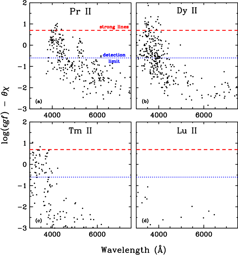
Figure 1: Relative strength plots for Pr II, Dy II, Tm II, and Lu II lines. Dashed lines in each box denote the approximate lower strength limit for strong lines, and dotted lines denote the lower limit for detectable lines, as defined in the text. For these plots the wavelength range has been restricted to $\lambda$ $>$ 3000 Å (the cutoff for ground-based spectra) and $\lambda$ $>$ 7500 Å (for lack of detectable lines of these species).

Almost all easily detectable RE lines are of low excitation, $\chi$ $\lesssim$ 1 eV, so the relative line strengths are not very sensitive to temperature. Choosing $\theta$ = 1.0 as a rough mean of the solar and stellar reciprocal temperatures, and adopting approximate solar abundance values for each element under consideration, we computed relative strength factors for Pr II, Dy II, Tm II, and Lu II lines, using the laboratory data that will be discussed in the appropriate subsections of §3. We did not perform such computations for Yb II, as it has only two very strong lines of interest for abundance analyses (see §3.4). The results of this exercise are displayed in Figure 1. With horizontal lines we mark the approximate minimum relative strength value for lines that can be considered “strong”. Such lines are those with evident saturation in their equivalent widths (EWs), which for the Sun empirically is log($EW/\lambda$) $\sim$ $-$5.3. We similarly mark the approximate strength value at which photospheric lines have log($EW/\lambda$) $\sim$ $-$6.5, too weak to be routinely used in abundance solar abundance analyses.

Figure 1 can be compared to similar plots for other RE elements in some of the previous papers of this series. Some general remarks apply to all RE ions. Most REs have complex energy structures, leading to large numbers of transitions. Their relative strength factors increase with decreasing wavelength; these usually are transitions from the lowest energy levels with the largest $\log gf$ values. The most fertile regime for RE transitions is the near-UV domain, $\lambda$ $<$ 4000 Å. Unfortunately, the strong-line density of all species increases in this wavelength range, and many promising RE transitions are hopelessly blended with (usually) Fe-peak lines. Finally, as is evident in Figure 1, very few RE ions have detectable transitions in the yellow-red ($\lambda$ $>$ 5000 Å) spectral region of the solar spectrum. Comments on the line strengths of individual species will be given in §3. These same strength factors turn out to work reasonably well for the $r$-process-rich giant stars. Their combination of cooler temperatures, more extended atmospheres, metal poverty, and enhanced $n$-capture abundances yields line strengths that are similar to or somewhat larger than those for the Sun.

We eliminated lines with relative strength factors that fell below the probable detection limits, and searched solar and stellar spectra for the remaining lines. In this effort we employed the large Kurucz (1998) line list, the solar line identifications of Moore, Minnaert, & Houtgast (1966), and the observed spectra described above. With these resources we were able to discard many additional lines that proved to be too weak and/or too blended to be of use either for the Sun or for the $r$-process-rich stars.

We then constructed synthetic spectrum lists for small spectral regions (4–6 Å) surrounding each promising candidate line. These lists were built beginning with the Kurucz (1998) atomic line database. We updated the $n$-capture species transition probabilities with results from this series of papers, including the laboratory data cited below for Pr, Dy, Tm, Yb, and Lu. We also used recently published $\log gf$ values for Cr I (Sobeck, Lawler, & Sneden 2007) and Zr II (Malcheva et al. 2006). Lines missing from the Kurucz database but listed in the laboratory studies or in the Moore et al. (1966) solar line atlas were added in. In spectral regions where molecular absorption is important, we used the Kurucz data for OH, NH, MgH, and CN, and Plez (private communication) data for CH.

We iterated the transition probabilities through repeated trial spectrum syntheses of the solar photosphere (and sometimes one of the $r$-process-rich giant stars). For the Sun, as in previous papers of this series we adopted the Holweger & Müller (1974) empirical model photosphere, and computed the synthetic spectra with the current version of Sneden’s (1973) LTE, 1-dimensional (1D) line analysis code MOOG. In these trial syntheses, no alterations were made to the lines with good laboratory $\log gf$’s. On occasion, obvious absorptions without plausible lab or solar identifications were arbitrarily defined to be Fe I lines with excitation energies $\chi$ = 3.5 eV and $\log gf$ values to match the photospheric absorption. We discarded all candidate RE lines that proved to be seriously blended with unidentified contaminants.

Final solar abundances for each line were determined through matches between the Delbouille et al. (1973) photospheric center-of-disk spectra and the empirically-smoothed synthetic spectra. The same procedures were applied to the observed stellar spectra (Table 1) and synthetic spectra generated with the model atmospheres whose parameters and their sources are given in Table 2.

3 ABUNDANCES OF PR, DY, TM, YB, AND LU

In this section we discuss our abundance determinations of elements Pr, Dy, Tm, Yb, and Lu in the Sun and the $r$-process-rich stars. Tables New Rare Earth Element Abundance Distributions for the Sun and Five $r$-Process-Rich Very Metal-Poor Stars, 4, and New Rare Earth Element Abundance Distributions for the Sun and Five $r$-Process-Rich Very Metal-Poor Stars contain the mean abundances in the solar photosphere and in the $r$-process-rich low metallicity giants for these elements and for other REs that have been analyzed in previous papers of this series. The full suite of elements will be discussed in §4. Table New Rare Earth Element Abundance Distributions for the Sun and Five $r$-Process-Rich Very Metal-Poor Stars also gives estimates of $r$-process abundance components in solar-system meteoritic material. These data will be discussed in more detail in §5.

3.1 Praseodymium

Pr ($Z$ = 59) has one naturally-occurring isotope, ¹⁴¹Pr. The Pr II spectrum has been well studied in the laboratory, with transition probabilities reported by Ivarsson et al. (2001; hereafter Iv01), Biémont et al. (2003) and Li et al. (2007; hereafter Li07), as well as numerous publications on its wide hyperfine structure. We will consider the hfs data in more detail in the Appendix.

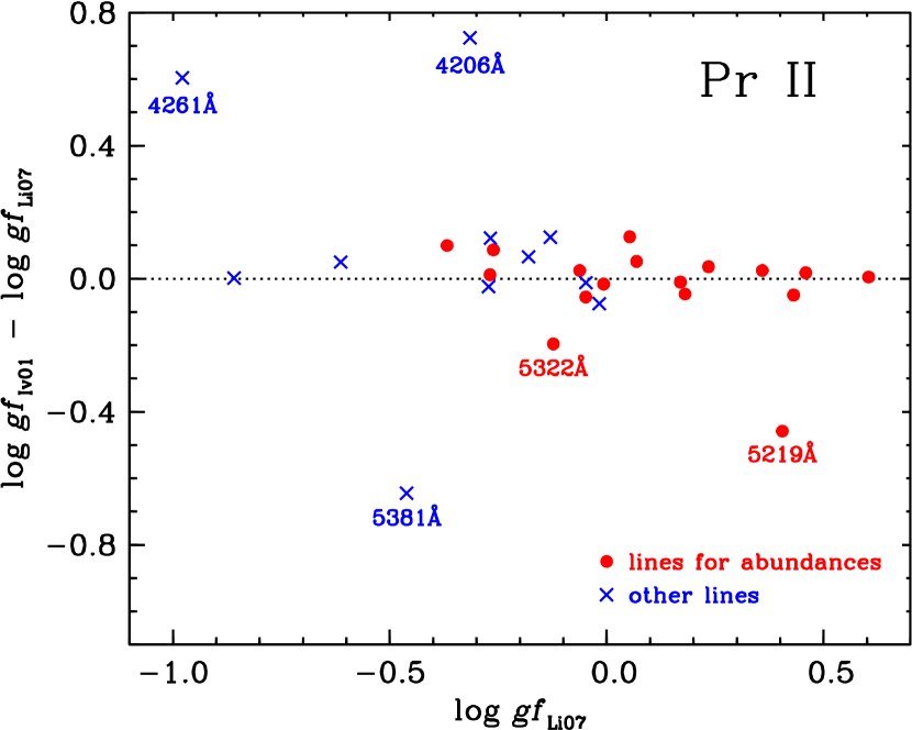
Figure 2: Differences between Ivarsson et al. (2001; Iv01) and Li et al. (2007; Li07) Pr II $\log gf$ values plotted as a function of wavelength. As indicated in the figure legend, red dots denote transitions employed in our solar/stellar analyses, and blue $\times$ symbols denote other lines in common between Iv01 and Li07.

We adopted Li07 as our primary transition probability source. This is the most recent and largest set, 260 lines, of purely experimental measurements (Li07 combined their own branching fractions with previously published lifetimes). Iv01 also conducted a smaller Pr II lab study, reporting $\log gf$values for 31 lines. However, their list includes four lines not published by Li07. Therefore we considered both Li07 and Iv01 data sets in our abundance determinations. In Figure 2 we plot the differences between individual Iv01 and Li07 $\log gf$ values, using different symbols to distinguish those lines employed in our abundance analyses from those that proved to be unsuitably weak or blended. There is generally good agreement: ignoring the five obviously discrepant lines that are labeled by wavelength in the figure, the mean difference is $<\mbox{$\log gf$}_{Iv01}-\mbox{$\log gf$}_{Li07}>$ = +0.03 $\pm$ 0.01 ($\sigma$ = 0.06, 23 lines). Comments on individual lines in common are given below. Biémont et al. (2003) also published $\log gf$’s for 150 Pr II lines. However, their values were determined by combining experimental Pr II lifetimes and theoretical branching fractions, which are very difficult to compute for the complex RE atomic structures (e.g., Lawler et al. (2008a).

Moore et al. (1966) give 21 Pr II identifications for the solar spectrum. However, most of them are very weak and/or blended. An early study by Biémont et al. (1979) has a good discussion of the benefits and disadvantages of many of these lines for photospheric abundance work. They used nine lines to derive log $\epsilon$(Pr)_⊙ = 0.71 $\pm$ 0.08, with individual lines contributing to the average with different weights. Only three of these lines were considered to be high-quality ones. More recently, Ivarsson, Wahlgren, & Ludwig (2003) employed synthetic/observed spectral matches to suggest log $\epsilon$(Pr)_⊙ = 0.4 $\pm$ 0.1, more than a factor of two smaller than the meteoritic value of log $\epsilon$(Pr)_met = 0.78 $\pm$ 0.03.

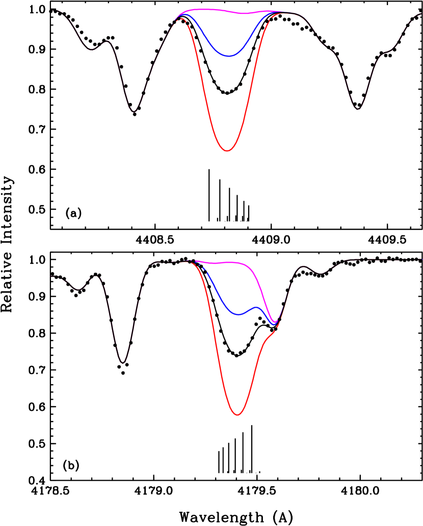
Figure 3: Observed and synthetic spectra in CS 31082-001 of two strong Pr II lines with wide hyperfine structure. In each panel, the points represent the observed spectrum. The magenta line is the spectrum computed with no contribution from Pr II; the black line is the best-fitting synthesis (with the Pr abundance given in Table 6; and the red and blue lines are the syntheses computed with Pr abundances altered by $\pm$0.3 dex from the best value. Vertical lines have been drawn at the bottom of each panel to indicate the wavelengths and relative strengths (arbitrary overall normalization) of the hyperfine components that comprise the Pr II transitions.

We searched for useful Pr II lines in the solar spectrum by first identifying them in CS 31082-001, which is the most extreme $r$-process-rich metal-poor star of our sample: [Fe/H] = –2.9, [Eu/Fe] = +1.6 (Hill et al. 2002). This star’s low metallicity and large [$n$-capture/Fe-peak] abundance ratios combine to yield many strong (and often essentially unblended) candidate transitions. Inspection of the CS 31082-001 spectrum yielded 43 lines from Li07 and an additional 3 lines from Iv01 that merited abundance consideration. Preliminary synthetic spectrum calculations suggested that 13 of these candidate lines were either too weak or too blended in both CS 31082-001 and the Sun. The wide hyperfine structure of all prominent Pr II lines made this exercise much easier than it would be in searches for lines with no hfs. In Figure 3 we illustrate this point with synthetic and observed spectra of the strong 4408.8 and 4179.4 Å transitions. Visual inspection of the Pr II profiles suggests that their full-width-half-maxima are FWHM $\simeq$ 0.4 Å, while observed and synthetic profiles of single lines (e.g., 4178.86 Å Fe II and 4179.59 Å Nd II) have FWHM $\simeq$ 0.25 Å

Wavelengths of the remaining useful Pr II lines are given in Table 6, along with their excitation energies and the Li07 and Iv01 transition probabilities. In Figure 2 one sees five lines with large $\log gf$ discrepancies between these studies. Three of the lines were not involved for our abundance studies and so we cannot comment further on them. Li07 caution that 5219.1 Å is blended on their spectra. We adopted the Iv01 value for this line. Finally, the difference between Iv01 and Li07 for 5322.8 Å is 0.2 dex, but abundances derived with the Li07 $\log gf$ proved to be consistent with those from other Pr lines.

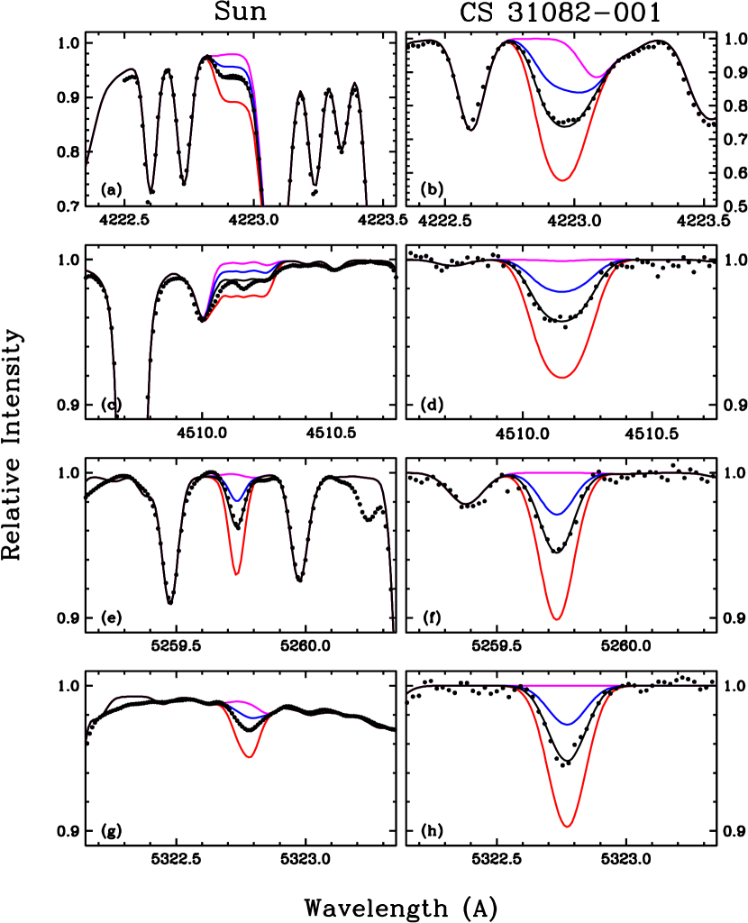
Figure 4: Observed and synthetic spectra of the Sun (left-hand panels (a), (c), (e), (g)) and CS 31082-001 (right-hand panels (b), (d), (f), (h)) for the four Pr II lines that contribute to the solar abundance estimate. In each panel, the points represent the observed spectrum. The magenta line is the spectrum computed with no contribution from Pr II; the black line is the best-fitting synthesis (with the Pr abundance given in Table 6); and the red and blue lines are the syntheses computed with Pr abundances altered by $\pm$0.3 dex from the best value. The solar spectrum is that of Delbouille et al. (1973), but sampled at a wavelength step size of 0.01 Å for display purposes.

We calculated solar photospheric synthetic spectra for all the Pr II lines of Table 6. We found, as have the previous studies cited above, that there are few useful solar Pr abundance indicators. Our final value was based on five lines (Table 6). We show the synthetic/observed photospheric spectrum matches for four of these lines in left-hand panels (a), (c), (e), and (g) of Figure 4, contrasting their appearance in right-hand panels (b), (d), (f), and (h) for CS 31082-001. We do not include the 5219.1 Å line in Figure 4 because it was too weak in the spectrum of CS 31082-001 to analyze in that star. Note that Li07 transition probabilities were used for the 4222.9, 4510.1, and 5322.8 Å lines and Iv01 values for the 5219.1 and 5259.7 Å lines. However, consistent abundances from all five lines were derived: the mean value (Table New Rare Earth Element Abundance Distributions for the Sun and Five $r$-Process-Rich Very Metal-Poor Stars) is log $\epsilon$(Pr)_⊙ = 0.76 $\pm$ 0.02 (sigma = 0.04). Our new photospheric abundance is in good agreement with the meteoritic and the Biémont et al. (1979) photospheric abundances that were quoted above.

For the $r$-process-rich low metallicity stars we derived abundances from 10–27 Pr II lines (Table 6). We plot the individual line abundances for these stars and the Sun as functions of wavelength in Figure 5, with their summary abundance statistics in the panel legends. In each case the line-to-line scatter was small, $\sigma$ $\simeq$ 0.06, and we found no significant abundance trends with wavelength, excitation energy (the range in this quantity is only $\simeq$1 dex), or $\log gf$.

3.2 Dysprosium

Dy ($Z$ = 66) has seven naturally-occurring isotopes, five of which contribute substantially to its solar-system abundance: ^156,158Dy, $\ll$1%, ¹⁶⁰Dy, 2.34%; ¹⁶¹Dy, 18.91%; ¹⁶²Dy, 25.51%; ¹⁶³Dy, 24.9%; and ¹⁶⁴Dy, 28.19% (Lodders 2003). The atomic structure of Dy II is complex, leading to a rich spectrum of transitions arising from low-excitation energy levels. This species has been well-studied in the laboratory recently, with published transition probabilities by Kusz (1992), Biémont & Lowe (1993), and Wickliffe, Lawler, and Nave (2000). The Wickliffe et al. study contains a detailed comparison of their transition probabilities with those of Kusz and Biémont & Lowe (as well as earlier investigations), and will not be repeated here.

We adopted the Wickliffe et al. (2000) $\log gf$ values, as in our earlier analyses of the $r$-process-rich stars. Those studies (e.g., Ivans et al. 2006 for HD 221170, and Sneden et al. 2003 for CS 22892-052) performed extensive searches for promising Dy II lines. However, the Dy abundances reported in those papers were derived from both EW matches and synthetic spectrum calculations. Therefore, to be internally consistent in our new analyses, we began afresh with new solar Dy II identifications and new synthesis line lists for each chosen feature. In principle Dy II lines should have both isotopic wavelength splitting and (for ^161,163Dy) hyperfine substructure. We inspected the profiles of many of the strongest lines appearing in National Solar Observatory (NSO) Fourier Transform Spectrometer (FTS) laboratory Dy II spectra. Some line substructure is present in each line. However, the components that are shifted away from the line centers are always very weak ($\lesssim$10% of central intensities), and the full widths near profile baselines are $\sim$0.05 Å. For all lines, FWHM $\sim$ 0.02 Å in the lab spectra. These widths are substantially smaller than the measured solar and stellar spectrum line widths. Therefore we treated all Dy II lines as single features.

There are many candidate lines, as indicated by their relative strength values shown in panel (b) of Figure 1. Solar Dy abundances could be determined from 13 of these transitions. The resulting mean photospheric abundance (Table New Rare Earth Element Abundance Distributions for the Sun and Five $r$-Process-Rich Very Metal-Poor Stars) is log $\epsilon$(Dy)_⊙ = +1.13 $\pm$ 0.02 ($\sigma$ = 0.06). This value is in excellent agreement with the meteoritic abundance, log $\epsilon$(Dy)_met = +1.13 $\pm$ 0.04 and with the Kusz (1992) photospheric abundance, log $\epsilon$(Dy)_⊙ = +1.14 $\pm$ 0.08. It is also in reasonable accord with the Biémont & Lowe (1993) value, log $\epsilon$(Dy)_⊙ = +1.20 $\pm$ 0.06.

Synthetic spectra of 24–35 lines were used in the Dy abundance derivations for the $r$-process-rich low-metallicity giants (Table 7). The analyses were straightforward, as many Dy II lines in each star’s spectrum were strong and unblended. This led to very well-determined mean abundances (Tables 4 and New Rare Earth Element Abundance Distributions for the Sun and Five $r$-Process-Rich Very Metal-Poor Stars).

3.3 Thulium

Tm ($Z$ = 69) has one naturally-occurring isotope, ¹⁶⁹Tm. This element is one of the least abundant of the REs: log $\epsilon$(Tm)_met = 0.11 $\pm$ 0.06 (Lodders 2003). Therefore Tm II transitions in solar and stellar spectra are weak, and relatively few can be employed in abundance analyses. Moore et al. (1966) list only 10 Tm II identifications in their solar line compendium; all of these lie at wavelengths $\lambda$ $<$ 4300 Å.

We considered the 146 Tm II lines investigated by Wickliffe & Lawler (1997). That study reported laboratory experimental transition probabilities derived from their branching fractions and the radiative lifetimes of Anderson, Den Hartog, and Lawler (1996). The relative strengths of these lines are displayed in panel (c) of Figure 1. Inspection of this plot suggests that few detectable Tm II lines will be found redward of 4000 Å, in accord with the Moore et al. (1966) identifications.

As in the case of Pr (§3.1), we began our search for suitable Tm II transitions with CS 31082-001, since they should stand out most clearly among the weaker Fe-peak contaminants in this star’s spectrum. Only nine lines were sufficiently strong and unblended to warrant further investigation. We computed synthetic spectra for each of these candidate features. Although Tm is an odd-$Z$, odd-$A$ atom with a non-zero nuclear spin ($I$ = $\frac{1}{2}$), inspection of the chosen Tm II lines in very high-resolution NSO FTS spectra showed that hyperfine splitting is very small, and could be safely ignored in the calculations.

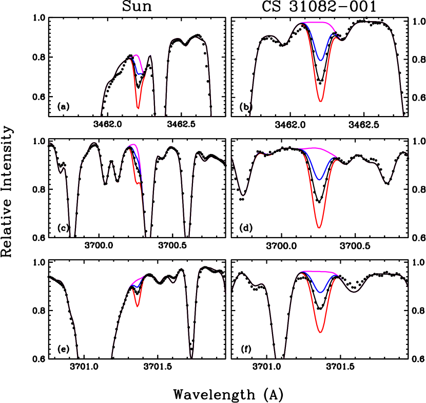
Figure 6: Observed and synthetic spectra of the Sun (left-hand panels (a), (c), (e)) and CS 31082-001 (right-hand panels (b), (d), (f)) for the three Tm II lines that contribute to the solar abundance estimate. In each panel, the points represent the observed spectrum. The magenta line is the spectrum computed with no contribution from Tm II; the black line is the best-fitting synthesis (with the Tm abundance given in Table 8); and the red and blue lines are the syntheses computed with Tm abundances altered by $\pm$0.3 dex from the best value. The solar spectrum is that of Delbouille et al. (1973), but sampled at a wavelength step size of 0.01 Å for display purposes.

Our synthetic spectra of Tm II lines for the solar photosphere showed that only three of them could be used for abundance analysis. The synthetic/observed spectrum matches for these lines in the solar photosphere are displayed in Figure 6, along with those for CS 31082-001. It is clear that each of these lines is weak and blended in the photospheric spectrum, while being much stronger and cleaner in the $r$-process-rich low metallicity giant star.

These lines and their photospheric abundances are listed in Table 8. We derive a formal mean abundance (Table New Rare Earth Element Abundance Distributions for the Sun and Five $r$-Process-Rich Very Metal-Poor Stars) of log $\epsilon$(Tm)_⊙ = +0.14 $\pm$ 0.02 ($\sigma$ = 0.04). Caution obviously is warranted here. Probably the $\sigma$ value is a truer estimate of the abundance uncertainty than the standard deviation of the mean. However, this photospheric abundance is in reasonable agreement with the meteoritic value, log $\epsilon$(Tm)_met = +0.11 $\pm$ 0.06.

More Tm II features could be employed in the abundance determinations for the $r$-process-rich low-metallicity giants (Table 8). Their mean values (Tables 4 and New Rare Earth Element Abundance Distributions for the Sun and Five $r$-Process-Rich Very Metal-Poor Stars) were based on 5–7 lines per star. For stars analyzed previously by our group, the new Tm abundances agree with the published values to within the uncertainty estimates. The Tm abundance for CS 31082-001will be discussed along with this star’s other REs in §4.2.

3.4 Ytterbium

Yb ($Z$ = 70) has seven naturally-occurring isotopes, six of which are major components of its solar-system abundance: ¹⁶⁸Yb, $\ll$1%; ¹⁷⁰Yb, 3.04%; ¹⁷¹Yb, 14.28%; ¹⁷²Yb, 21.83%; ¹⁷³Yb, 16.13%; ¹⁷⁴Yb, 31.83%; and ¹⁷⁶Yb, 12.76% (Lodders 2003). The atomic structure of Yb II is similar to that of Ba II, with a ²S ground state and first excited state more than 2.5 eV above the ground state. Therefore this species has very strong resonance lines at 3289.4 and 3694.2 Å as the only obvious spectral signatures of this element. All other Yb II lines are expected to be extremely weak.

The Yb II resonance lines have complex hyperfine and isotopic substructures that broaden their absorption profiles by 0.06 Å and must be included in synthetic spectrum computations. In the Appendix we discuss the literature sources for the resonance lines and tabulate their substructures in a form useful for stellar spectroscopists. Moore et al. (1966) identified major Fe I, Fe II, and V II contaminants to the 3289.4 Å line, and our synthetic spectra confirmed that Yb II is a small contributor to the total feature. From our synthetic spectra of the 3694.2 Å line we derived log $\epsilon$(Yb)_⊙ = +0.86 $\pm$ 0.10 (Table New Rare Earth Element Abundance Distributions for the Sun and Five $r$-Process-Rich Very Metal-Poor Stars), in reasonable agreement with log $\epsilon$(Yb)_met = +0.94 $\pm$ 0.03. The large uncertainty attached to our photospheric abundance arises from a variety of sources: (a) reliance on a single Yb II line; (b) its large absorption strength, which increases the dependence on adopted microturbulent velocity; (c) the contaminating presence of the strong Fe I 3694.0 Å line; and (b) closeness of this spectral region to the Balmer discontinuity.

We then synthesized the 3289 and 3694 Å lines in the stellar spectra. However, these are $r$-process-rich stars, and the isotopic mix in a pure $r$-process nucleosynthetic mix is different than that of the solar system ($r$-process and $s$-process) combination. For our computations we adopted (see Sneden et al. 2008): ^168,170Yb, 0.0%; ¹⁷¹Yb, 17.8%; ¹⁷²Yb, 22.1%; ¹⁷³Yb, 19.0%; ¹⁷⁴Yb, 22.7%; and ¹⁷⁶Yb, 18.4%.

The Yb contribution to the 3289 Å feature is very large in the $r$-process-rich stars. In the most favorable case, CS 31082-001, Yb accounts for roughly 75% of the total blend. Unfortunately, the contributions of the contaminants (mostly V II) cannot be assessed accurately enough for this line to be a reliable Yb abundance indicator. The synthetic/observed spectral matches of the 3694 Å line provide the new Yb abundances listed in Tables 4 and New Rare Earth Element Abundance Distributions for the Sun and Five $r$-Process-Rich Very Metal-Poor Stars. These values are consistent with the ones reported in the original papers on these stars. However, while the Yb II absorption dominates that of the possible metal-line contaminants, the Balmer lines in this spectral region are substantially stronger in these low-pressure giant stars than they are in the solar photospheric spectrum. In particular, H I lines at 3691.6 and 3697.2 Å significantly depress the local continuum at the Yb II wavelength. Caution is warranted in the interpretation of these Yb abundances.

3.5 Lutetium

Lu ($Z$ = 71), has two naturally-occurring isotopes: ¹⁷⁵Lu, 97.416%; and ¹⁷⁶Lu, 2.584% (Lodders 2003). It is the least abundant RE: log $\epsilon$(Lu)_met = 0.09 $\pm$ 0.06 (Lodders). Lu II has a relatively simple structure, with a ¹S ground state. It has no other very low-energy states; the first excited level lies 1.5 eV above the ground state. This ion with only two valence electrons has relatively few strong lines in the visible and near UV connected to low E.P. levels, although most of the prominent lines have well-determined experimental transition probabilities.

We considered only the Lu II transitions of Quinet et al. (1999), using their experimental branching fractions and lifetime measurements by Fedchak et al. (2000) to determine Lu II transition probabilities. These are are listed, along with wavelengths and excitation energies, in Table 12 of Lawler et al. (2009). The combination of a small solar-system Lu abundance and the (unfavorable) atomic parameters produces very small relative strength factors for these lines, as shown in panel (d) of Figure 1. No line even rises to our defined “weak-line” threshold of usefulness. Moore et al. (1966) lists only 3077.6, 3397.1, and 3472.5 Å Lu II identifications in their solar line compendium, and all of these lines appear to be blended.

We made a fresh search for detectable lines of Lu II, and succeeded mainly in confirming the results of a previous investigation by Bord, Cowley, & Mirijanian (1998). Those authors argued that all of the lines identified by Moore et al. (1966) are unsuitable for solar Lu abundance work. They quickly dismissed the 3077.6 and 3472.5 Å lines and performed an extended analysis of 3397.1 Å. Synthetic spectrum computations around this feature (see their Figures 2 and 3) convinced them that molecular NH dominates the absorption at the Lu II wavelength. Our own trials produced the same outcome.

Bord et al. (1998) detected Lu II 6221.9 Å in the Delbouille et al. (1973) photospheric spectrum. This line is extremely weak, EW $\sim$ 1 mÅ, and its hyperfine substructure spreads the absorption over $\sim$0.5 Å. The complex absorption profile of this line (see their Figure 4) actually increases one’s confidence in its identification in the photospheric spectrum. Bord et al. reported log $\epsilon$(Lu)_⊙ = +0.06 with an estimated $\pm$0.10 uncertainty from this line.

We repeated their analysis, using the hyperfine substructure pattern given in Table 13 of Lawler et al. (2009), and derived log $\epsilon$(Lu)_⊙ = +0.12 $\pm$ 0.08 (Table New Rare Earth Element Abundance Distributions for the Sun and Five $r$-Process-Rich Very Metal-Poor Stars), where the error reflects uncertainties in matching synthetic and observed feature profiles. This photospheric abundance is consistent with the Bord et al. (1998) value and with the meteoritic abundance quoted above, given the uncertainties attached to each of these estimates. Our lack of success in identifying other Lu abundance indicators in the solar photospheric spectrum suggests that prospects are poor for reducing its error bar substantially in the future.

We also attempted to study the 3397 and 6621 Å lines in our sample of $r$-process-rich low metallicity giants. Absorption by Lu II at 3397.1 Å is certainly present in the spectra of at least CS 22892-052 and CS 31082-001. Unfortunately, the lower resolutions of our stellar spectra compared to that of the solar spectrum creates more severe blending of the Lu transition with neighboring lines, and NH contamination of the total feature still creates substantial abundance ambiguities. The 6221.9 Å line should be present, albeit very weak, in these stars. However, our spectra (when they extend to this wavelength range) lack the S/N to allow meaningful detections. We therefore cannot report Lu abundances for these $r$-process-rich stars.

4 RARE EARTH ABUNDANCE DISTRIBUTIONS IN THE SUN AND R-PROCESS-RICH STARS

4.1 The Sun and Solar System

With new analyses of Pr, Dy, Tm, Yb, and Lu we now have determined abundances for the entire suite of REs in the solar photosphere. In Table New Rare Earth Element Abundance Distributions for the Sun and Five $r$-Process-Rich Very Metal-Poor Stars we merge the results of this and our previous papers. Missing from the list is of course Pm (Z = 61), whose longest-lived isotope, ¹⁴⁵Pm, is only 17.7 years (Magill, Pfennig, and Galy 2006). We also chose not to include a photospheric value for Ba, whose few transitions are so strong that their solar absorptions cannot be reliably modeled in the sort of standard photospheric abundance analysis that we have performed.

The photospheric abundance uncertainties quoted in Table New Rare Earth Element Abundance Distributions for the Sun and Five $r$-Process-Rich Very Metal-Poor Stars are combinations of internal “scatter” factors (mainly continuum placement, observed/synthetic matching, and line blending problems) and external “scale” factors (predominantly solar model atmosphere choices). These issues are discussed Lawler et al. (2009) and in previous papers of this series. We remind the reader that our abundance computations have been performed with the traditional assumptions of LTE and 1D static atmosphere geometry. Very little has been done to date to explore the effects of these computational limitations for RE species in the solar atmosphere. Mashonkina & Gehren (2000) have performed non-LTE abundance analyses of Ba and Eu, but their photospheric abundances are not substantially different from LTE results. There have been efforts to model the solar spectrum with more realistic 3-dimensional (3D) hydrodynamic models; see the summary in Grevesse, Asplund, & Sauval (2007), and references therein. These studies so far have reported new solar abundances only for the lighter elements (CNO, Na$-$Ca, and Fe). Generally the 3D non-LTE line modeling efforts yield lower abundances: comparing the photospheric values in Grevesse et al. to those of the older standard compilation of Anders & Grevesse (1989), $<\delta$log $\epsilon>$ = $-$0.12 $\pm$ 0.03 ($\sigma$ = 0.09, for 11 elements that can be studied with photospheric spectra). We thus expect that any RE abundance shifts with 3D modeling would be similar from element to element, leaving their abundance ratios essentially unchanged. Future studies to explore these effects in detail will be welcome.

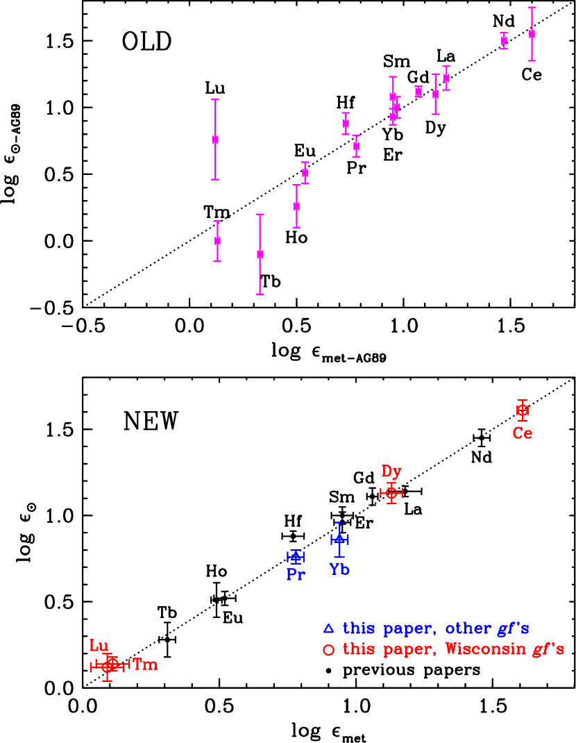
Figure 7: Comparisons of solar-system meteoritic and solar photospheric abundances of the RE elements. In the top panel, the “OLD” abundances are the recommended values from two decades ago (Anders & Grevesse 1989). In the bottom panel, the “NEW” meteoritic values are from (Lodders 2003), and the solar photospheric abundances are from in this study and previous papers of this series. We separate the new photospheric results into three groups, using red open circles to denote those elements whose abundances are based on transition probabilities published by the Wisconsin group, blue open triangles for those elements whose abundances are based on other sources for the transition probabilities, and black dots for abundances determined in earlier papers of this series.

In Figure 7 we compare RE photospheric abundances to their meteoritic values. In the top panel the “OLD” values are best estimates by Anders & Grevesse (1989). While the average agreement is good, significant discrepancies between individual abundances are evident, particularly at the low-abundance end. Formally, a simple mean is $<\log\epsilon_{\odot-AG89}-\log\epsilon_{met-AG89}>$ = 0.00 $\pm$ 0.06 ($\sigma$ = 0.22). In the bottom panel, the “NEW” meteoritic abundances (Lodders 2003) are correlated with our “NEW” photospheric ones (Table New Rare Earth Element Abundance Distributions for the Sun and Five $r$-Process-Rich Very Metal-Poor Stars). The data sources are denoted by different symbols in the figure: red open circles for photospheric abundances newly determined here and in Lawler et al. (2009) for which Wisconsin-group lab data have been used; black filled circles for abundances reported in our previous papers; and blue open triangles for two elements with transition probability data adopted from other literature sources. Clearly the agreement is excellent: for 15 elements the formal mean difference is $<\log\epsilon_{\odot}-\log\epsilon_{met}>$ = 0.01 $\pm$ 0.01 ($\sigma$ = 0.05). No trends are discernible with the source of atomic data, or the abundance levels (as shown in the figure), or the number of lines that contribute to the photospheric abundances (Table New Rare Earth Element Abundance Distributions for the Sun and Five $r$-Process-Rich Very Metal-Poor Stars). With the possible exception of Hf (discussed in Lawler et al. 2007 and in §5), and with repeated cautions about the photospheric abundances deduced from only one or two transitions, the two primary sources of primordial Solar-System abundances appear to be in complete accord.

4.2 The $r$-process-Rich Low Metallicity Giant Stars

Rare-earth abundances for the five $r$-process-rich stars from this and our previous papers are collected in Tables 4 and New Rare Earth Element Abundance Distributions for the Sun and Five $r$-Process-Rich Very Metal-Poor Stars. For all stars the Pr, Dy, Tm, and Yb abundances are, of course, newly determined in this paper. We chose also to redo all the Ba abundances via new synthetic spectrum calculations, to ensure that these were determined in a consistent manner. We also performed new analyses for selected elements in individual stars (e.g., Tb in HD 115444) when the original papers either did not report abundance values or did so with now-outdated atomic data.

Of particular interest is the very $n$-capture-enhanced star CS 31082-001, which is a recent addition to our $r$-process-rich star list. This star gained notoriety as the first $r$-process-rich star with a convincing detection of U, a long-lived radioactive element of great interest to cosmochronology (Cayrel et al. 2001). The first and most complete study of this star was published by Hill et al. (2002). The mean difference between our RE abundances for this star and theirs is $<\log\epsilon_{Hill}-\log\epsilon_{us}>$ = $-$0.05 $\pm$ 0.03 ($\sigma$ = 0.10, 12 elements in common). We also compared our CS 31082-001 abundances with those of Honda et al. (2004), with similar results: $<\log\epsilon_{Honda}-\log\epsilon_{us}>$ = +0.07 $\pm$ 0.03 ($\sigma$ = 0.09, 12 elements in common). The mean offsets are very small, and reflect minor differences in model atmospheres, observed spectra, analytical techniques, and atomic data choices. The element-to-element scatters are also reasonable, given the use of many more transitions in our study (a total of 342, Table 4) compared to 95 in Hill et al. and 49 in Honda et al. Note that some portion of the $\sigma$’s in these comparisons arises because the Tb abundance differences are offset by $\simeq$0.2 dex from the mean differences (we derive larger values). Investigation of this one anomaly is beyond the scope of this work.

The abundance standard deviations of samples ($\sigma$) and of means that are given in Tables 4 and New Rare Earth Element Abundance Distributions for the Sun and Five $r$-Process-Rich Very Metal-Poor Stars refer to internal (measurement scatter) errors only. To investigate scale uncertainties, we determined the abundance sensitivities of eight RE elements to changes in model parameters (T_eff, log g, [M/H], $\xi_{\rm t}$), to changes in the adopted model atmosphere grid, and to changes to line computations to better account for continuum scattering opacities. In Table 9 we summarize the results of these exercises. We began with a “baseline” model atmosphere from the Kurucz (1998) grid with parameters T_eff = 4750 K, log g = 1.5, [M/H] = –2.5, and $\xi_{\rm t}$ = 2.0. Such a model is similar to the ones adopted for the $r$-process-rich giants (Table 2). We derived abundances with this model for 1-4 typical transitions each of the elements for the program star CS 31082-001. Full account was taken of hyperfine and isotopic substructure for La, Pr, Eu, and Yb. We then repeated the abundance derivations for models with parameters varied as indicated in Table 9, including a trial using a model with baseline parameters taken from the new MARCS (Gustafsson et al. 2008) grid. The inclusion of scattering in computations of continuum source functions, a new feature in our analysis code, is described in Sobeck et al. (2008)

The Table 9 quantities are differences between abundances of the individual models and those of the baseline model. The uncertainties in stellar model parameters given in the original $r$-process-star papers are typically $\pm$150 K in T_eff, $\pm$0.3 in log g, $\pm$0.2 km s^-1 in $\xi_{\rm t}$, and $\pm$0.2 in [M/H] metallicity. Application of these uncertainties to the model parameter dependences of Table 9 suggests that [M/H] and $\xi_{\rm t}$ choices are not important abundance error factors. Temperature and gravity values obviously play larger roles. However, while the absolute abundances of individual elements change with different T_eff and log g choices, the relative abundances generally do not; in most cases, all RE abundances move in lock step. Assuming here that the atmosphere parameter uncertainties are uncorrelated, we estimate total abundance uncertainties for each RE element to be $\sim$0.15$-$0.20, but the abundance ratios have uncertainties of $\sim$0.01$-$0.05 (the exception is Yb, represented by only one very strong line in the UV spectral region; see §3.4). More detailed computations that consider departures from LTE among RE first ions in the atmospheres of very metal-poor giant stars should be undertaken in the future. Some first steps in this direction have been undertaken for Ba and Eu by Mashonkina et al. (2008), but such calculations will need to be repeated for many REs to understand the magnitude of corrections to the abundances reported here.

5 DISCUSSION

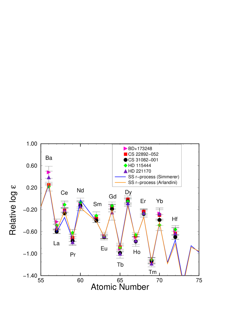
Figure 8: Comparison of the newly derived RE abundances in five r-rich halo stars with predictions for solar system r-process only abundances from Arlandini et al. (1999) and Simmerer et al. (2004). For each star the abundances have been normalized at Eu.

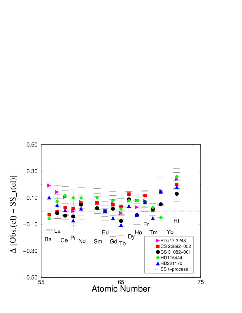
Figure 9: Comparison of the newly derived RE abundances in five r-rich halo stars to the solar system r-process only value from Arlandini et al. (1999). For each star the abundances have been normalized at Eu. The dotted line indicates a perfect agreement between the stellar and solar system r-only values. The error bars are the sigma values listed for each star in Tables 4 and New Rare Earth Element Abundance Distributions for the Sun and Five $r$-Process-Rich Very Metal-Poor Stars.

We illustrate the RE abundances for BD+17 3248, CS 22892-052, CS 31082-001, HD 115444 and HD 221170 in Figures 8 and 9. For each star the abundances have been normalized at Eu, a predominantly $r$-process element. In Figure 8 these relative abundances are shown in comparison to the Solar System $r$-process-only predictions from Arlandini et al. (1999) and Simmerer et al. (2004). We note first the excellent star-to-star (relative abundance) agreement. Early RE abundance distributions of $n$-capture-rich metal-poor stars indicated large star-to-star scatter for a number of individual elements (e.g., Luck & Bond 1985, Gilroy et al. 1988). The combination of substantially better S/N and resolution of the stellar spectra and the experimental initiatives of this series of papers has dramatically reduced that scatter – all the RE elements are now in very good (relative) agreement for these five halo stars.

Figure 8 also uses solid lines to illustrate the solar-system $r$-process-only meteoritic abundances determined by Simmerer et al. (2004) and Arlandini et al. (1999). In both cases, these values were computed by subtracting the $s$-process-only abundances from the total elemental abundances. The “classical” method (Simmerer et al.) matches smooth $\sigma$N_s curves to those isotopes of $n$-capture elements whose production is essentially all due to the $s$-process, and infers from those empirical curves the $s$-process amounts of elements that can be produced by both the $r$-process and $s$-process. The solar system $r$-process abundances are then just the residuals between total elemental and $s$-process amounts. The “stellar” method (Arlandini et al.) uses theoretical models of $s$-process nucleosynthesis instead of empirical $s$-process abundance curves, and again infers the $r$-process amounts by subtraction.

Our stellar abundances compare very well with the relative solar system $r$-process distributions. In the past we and other investigators have found overall agreement, but on a more approximate scale. The new abundance determinations shown in Figure 8 tighten the comparison, with deviations between the stellar and solar system r-process curves of typically less than 0.1 dex – probably the practical limit of what is currently possible. These abundance comparisons strongly support many other studies (see Sneden et al. 2008, and references therein) arguing that essentially the same process was responsible for the formation of all of the $r$-process contributions to these elements early in the history of the Galaxy in the element progenitor stars to the presently-observed $r$-process-rich halo stars.

Despite this general level of elemental abundance consistency, there are some interesting deviations. In particular, the two solar system $r$-process predictions differ by about 0.1 dex for the elements Ce and Nd (Table New Rare Earth Element Abundance Distributions for the Sun and Five $r$-Process-Rich Very Metal-Poor Stars). In both cases the stellar model predictions from Arlandini et al. (1999) give a better fit to the stellar abundance data than do the standard model predictions from Simmerer et al. (2004). This suggests that the Arlandini et al. $r$-process distribution might be superior for such abundance comparisons. This has been noted previously by others (e.g., Roederer et al. 2008) for isotopic studies.

There is also still some star-to-star scatter particularly at Ba, with several stellar elemental abundances appearing somewhat higher than the solar system r-process curves. This can be seen more clearly in Figure 9, where we illustrate the difference between the relative (scaled to Eu) stellar RE and the scaled solar system r-process abundances (Arlandini et al. 1999) in the five $r$-process-rich stars. While most of the individual elemental abundance data lie close to the dotted line (indicating perfect agreement with the solar $r$-process), Ba and Yb have significant star-to-star scatter. But both elements have inherent observational problems, as they are represented by only a few very strong transitions that have multiple isotopic components whose relative abundances are sensitive to the relative $r$-/$s$-process dominance (recall the Yb discussion in 3.4). Abundance determinations for Yb and Ba are less reliable than those of most other RE elements, and should be treated with caution.

We also note that for BD+17 3248 the RE abundances relative to Eu appear to be somewhat higher their values in the other stars, particularly for the predominantly $s$-process elements Ba and La. BD+17 3248 has a metallicity of [Fe/H] $\simeq$ –2.1 (Cowan et al. 2002), so this star might be showing the signs of the onset of Galactic $s$-processing, which occurs at approximately that metallicity (Burris et al. 2000). On the other hand HD 221170 with a similar metallicity (Ivans et al. 2006) does not seem to show the same deviations for the $s$-process elements, and thus the deviations for BD+17 3248 may be specific to that star.

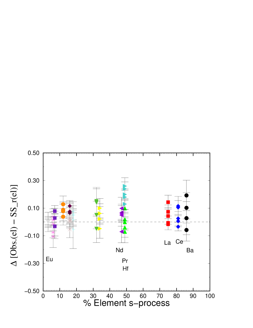
Figure 10: Comparison of the newly derived RE abundances in five r-rich halo stars to the solar system r-process only value from Arlandini et al. (1999) as a function of percentage of the solar system elemental s-process. The dashed line indicates a perfect agreement between the stellar and solar system r-only values. For clarity in this figure, a different color has been used for each element.

We examine whether there is any correlation between the deviation of the stellar abundances from the solar system r-process values and the $s$-process percentage of those elements in solar system material (from Simmerer et al. 2004) in Figure 10. It is clear that there is little if any secular trend with the abundance differences with increasing solar-system $s$-process abundance percentage. This lack of correlation was also found specifically for the element Ce by Lawler et al. (2009).

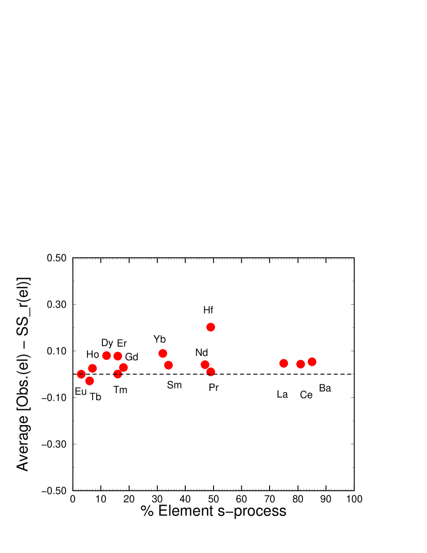
Figure 11: Averages of the stellar elemental abundance offsets of the five stars with respect to the solar system r-process only value from Arlandini et al. (1999) as a function of percentage of the solar system elemental s-process. For each star included in the average the abundance offsets have been normalized at Eu. The dotted line indicates a perfect agreement between the average stellar and solar system r-only values.

To get a clearer sense of the overall abundance agreement with the solar-system $r$-process abundances, we show in Figure 11 the arithmetic averages of the elemental abundance offsets (from Figure 10) for the five stars, again as a function of $s$-process percentage. Obviously these average offsets with respect to the solar-system $r$-process values are very small. Including all elements the mean of the average offsets is $\log\epsilon$ = 0.05 ($\sigma$ = 0.05). Previously Lawler et al. (2007) had found that the observed average stellar abundance ratio of Hf/Eu in a group of metal-poor halo stars is larger than previous estimates of the solar-system $r$-process-only value, suggesting a somewhat larger contribution from the $r$-process to the production of Hf. Our new analysis supports that finding, as the average Hf offset is larger than all of the other elemental abundances. If the solar system $r$-process contribution was larger it would drive down the average offset illustrated in Figure 11. Ignoring the Hf results, the mean of the average offsets for all of the other RE elements is 0.04 ($\sigma$ = 0.03). This is essentially a perfect agreement within the limits of our observational and experimental uncertainties, as well as the uncertainties (observational and theoretical) associated with the solar system $r$-process-only abundance values.

6 CONCLUSIONS

We have determined new abundances of Pr, Dy, Tm, Yb, and Lu for the solar photosphere and for five very metal-poor, $r$-process-rich giant stars. Combining these results with those of previous papers in this series (cited in §1), we have now derived very accurate solar/stellar abundances for the entire suite of stable RE elements.

With the single exception of Hf, the solar photospheric abundances agree with solar-system meteoritic values perfectly to within the uncertainty estimates of each. Our photospheric and stellar analyses have emphasized studying as many transitions of each species as possible (up to 46 Nd II lines in the Sun, up to 72 Sm II lines in BD+17 3248). The line-to-line abundance scatters are always small when the number of available transitions is large (typically $\sigma$ $<$ 0.07). This clearly demonstrates the reliability of the RE transition probabilities published in this series of papers. We argue that, with proper care in stellar analyses, trustworthy abundances of RE elements can be now be determined from spectra in which far fewer transitions are available.

Utilizing the new experimental atomic data we have determined far more precise stellar RE elemental abundances in five $r$-process rich stars. These newly derived values show a dramatic decrease in star-to-star elemental abundance scatter – all the RE elements are now in very good (relative) agreement for these five halo stars. Furthermore, our newly derived values indicate an almost perfect agreement between the average stellar abundances and the solar system $r$-process-only abundances for a wide range of elements in these five $r$-process-rich stars. There is no evidence for significant $s$-process contamination. The one exception appears to be a somewhat higher value of stellar Hf with respect to the solar system $r$-process-only value for this element. This may indicate that further analysis of the solar $r$- and $s$-process deconvolution for this element might be useful. These results for the five $r$-process-rich halo stars confirm, and strongly support, early studies that indicate that the r-process was dominant for the $n$-capture elements early in the history of the Galaxy.

Figure 5: Derived Pr abundances for the Sun and the $r$-process-rich low metallicity stars plotted as functions of wavelength. The abundance range shown for each star is 0.6 dex, and is centered vertically on the mean abundance, which is indicated with a dotted line. The legend of each panel records this abundance mean, along with the sample standard deviation and number of transitions used.

Table 1: Spectroscopic Observations

Spectrograph	$\lambda$ Range	$R$	$S/N$	$F$	$\lambda_{app}$	Stars
	Å				Å
Keck I HIRES	3050–5950	40,000	100	1142	3500	CS 31082-001, HD 221170
			150	1500	4000	CS 31082-001, HD 221170
			200	1778	4500	CS 31082-001, HD 221170
	3100–4250	45,000	100	1286	3500	CS 22892-052
			150	1688	4000	CS 22892-052
			200	2000	4500	CS 22892-052
	3100–4650	45,000	100	1286	3500	BD+17 3248, HD 115444
			150	1688	4000	BD+17 3248, HD 115444
			200	2000	4500	BD+17 3248, HD 115444
McDonald “2d-coude”	3800–9000	60,000	100	1500	4000	BD+17 3248, HD 115444
			250	2500	6000	BD+17 3248, HD 115444
	3800–7800	60,000	80	1200	4000	HD 221170
			275	2750	6000	HD 221170
	4200–7000	60,000	50	750	4000	CS 22892-052
			150	1500	6000	CS 22892-052
Magellan Clay MIKE	3800–4950	50,000	100	1250	4000	CS 22892-052
	5050–8000	38,000	150	950	6000	CS 22892-052

Table 2: Stellar Model Parameters

Star	Teff	log $g$	[Fe/H]	vt	Reference
	K			km s-1
BD+17 3248	5200	1.80	$-$2.10	1.90	Cowan et al. (2002)
CS 22892-052	4800	1.50	$-$3.12	1.95	Sneden et al. (2003)
CS 31082-001	4825	1.50	$-$2.91	1.90	Hill et al. (2002)
HD 115444	4800	1.50	$-$2.90	2.00	Westin et al. (2000)
HD 221170	4510	1.00	$-$2.19	1.80	Ivans et al. (2006)

Table 3: Solar Rare Earth Abundances

Element	Z	$\log\epsilon_{met}$	$\log\epsilon_{\odot}$	$\sigma$	#	Ref	$\log N_{r}$	$\log N_{r}$
		meteoritic					empirical	stellar
Ba	56	2.19 $\pm$ 0.03	$\cdots$	$\cdots$	$\cdots$	1	–0.0936	–0.0696
La	57	1.18 $\pm$ 0.06	1.14 $\pm$ 0.01	0.03	14	2	–0.9547	–0.9210
Ce	58	1.61 $\pm$ 0.02	1.61 $\pm$ 0.01	0.06	45	3	–0.6904	–0.5733
Pr	59	0.78 $\pm$ 0.03	0.76 $\pm$ 0.02	0.04	5	1	–1.0862	–1.0670
Nd	60	1.46 $\pm$ 0.03	1.45 $\pm$ 0.01	0.05	46	4	–0.3723	–0.5163
Sm	62	0.95 $\pm$ 0.04	1.00 $\pm$ 0.01	0.05	36	5	–0.7595	–0.7592
Eu	63	0.52 $\pm$ 0.04	0.52 $\pm$ 0.01	0.04	14	6	–1.0424	–1.0376
Gd	64	1.06 $\pm$ 0.02	1.11 $\pm$ 0.01	0.05	20	7	–0.5591	–0.5546
Tb	65	0.31 $\pm$ 0.03	0.28 $\pm$ 0.07	0.10	2	8	–1.2218	–1.2526
Dy	66	1.13 $\pm$ 0.04	1.13 $\pm$ 0.02	0.06	13	1	–0.4437	–0.4755
Ho	67	0.49 $\pm$ 0.02	0.51 $\pm$ 0.10	0.10	3	9	–1.0899	–1.0862
Er	68	0.95 $\pm$ 0.03	0.96 $\pm$ 0.03	0.06	8	10	–0.6798	–0.6832
Tm	69	0.11 $\pm$ 0.06	0.14 $\pm$ 0.02	0.04	3	1	–1.5086	–1.4841
Yb	70	0.94 $\pm$ 0.03	0.86 $\pm$ 0.10	0.10	1	1	–0.7889	–0.7783
Lu	71	0.09 $\pm$ 0.06	0.12 $\pm$ 0.08	0.08	1	1	–1.5100	–1.5317
Hf	72	0.77 $\pm$ 0.04	0.88 $\pm$ 0.02	0.03	4	11	–1.0974	–1.1675

References. — 1. This paper; 2. Lawler et al. (2001a); 3. Lawler et al. (2009); 4. Den Hartog et al. (2003); 5. Lawler et al. (2006); 6. Lawler et al. (2001c); 7. Den Hartog et al. (2006); 8. Lawler et al. (2001b); 9. Lawler et al. (2004); 10. Lawler et al. (2008b); 11. Lawler et al. (2007)

Table 4: Rare Earth Abundances for BD+17 3248, CS 22892-052, and CS 31082-001

		BD+17 3248				CS 22892-052				CS 31082-001
El	Z	$\log\epsilon$	$\sigma$	#	Ref	$\log\epsilon$	$\sigma$	#	Ref	$\log\epsilon$	$\sigma$	#	Ref
Ba	56	+0.48 $\pm$ 0.05	0.11	4	1	–0.01 $\pm$ 0.06	0.12	4	1	$\cdots$	$\cdots$	$\cdots$	1
La	57	–0.42 $\pm$ 0.01	0.05	15	2	–0.84 $\pm$ 0.01	0.05	15	2	–0.62 $\pm$ 0.01	0.04	9	2
Ce	58	–0.11 $\pm$ 0.01	0.05	40	4	–0.46 $\pm$ 0.01	0.05	32	4	–0.29 $\pm$ 0.01	0.03	38	4
Pr	59	–0.71 $\pm$ 0.02	0.06	18	1	–0.96 $\pm$ 0.02	0.07	15	1	–0.79 $\pm$ 0.01	0.07	27	1
Nd	60	–0.09 $\pm$ 0.01	0.06	57	5	–0.37 $\pm$ 0.01	0.06	37	5	–0.15 $\pm$ 0.01	0.08	68	1
Sm	62	–0.34 $\pm$ 0.01	0.05	72	6	–0.61 $\pm$ 0.01	0.07	55	6	–0.42 $\pm$ 0.01	0.04	67	1
Eu	63	–0.68 $\pm$ 0.01	0.04	9	1	–0.95 $\pm$ 0.01	0.02	9	1	–0.72 $\pm$ 0.01	0.03	7	1
Gd	64	–0.14 $\pm$ 0.01	0.04	41	7	–0.42 $\pm$ 0.01	0.07	32	7	–0.21 $\pm$ 0.01	0.05	32	1
Tb	65	–0.91 $\pm$ 0.02	0.05	5	8	–1.13 $\pm$ 0.01	0.04	7	9	–1.01 $\pm$ 0.01	0.04	9	1
Dy	66	–0.04 $\pm$ 0.01	0.05	28	1	–0.26 $\pm$ 0.01	0.06	29	1	–0.07 $\pm$ 0.01	0.05	35	1
Ho	67	–0.70 $\pm$ 0.02	0.05	11	10	–0.92 $\pm$ 0.01	0.02	13	10	–0.80 $\pm$ 0.03	0.09	12	1
Er	68	–0.25 $\pm$ 0.01	0.04	17	11	–0.48 $\pm$ 0.01	0.04	21	11	–0.30 $\pm$ 0.01	0.04	19	11
Tm	69	–1.12 $\pm$ 0.02	0.05	6	1	–1.39 $\pm$ 0.02	0.04	6	1	–1.15 $\pm$ 0.02	0.06	7	1
Yb	70	–0.27 $\pm$ 0.10	0.10	1	1	–0.55 $\pm$ 0.10	0.10	1	1	–0.41 $\pm$ 0.10	0.10	1	1
Lu	71	$\cdots$	$\cdots$	$\cdots$	1	$\cdots$	$\cdots$	$\cdots$	1	$\cdots$	$\cdots$	$\cdots$	1
Hf	72	–0.57 $\pm$ 0.03	0.08	6	2	–0.88 $\pm$ 0.01	0.04	8	2	–0.72 $\pm$ 0.01	0.04	10	2

Table 5: Rare Earth Abundances for HD 115444 and HD 221170

		HD 115444				HD 221170
El	Z	$\log\epsilon$	$\sigma$	#	Ref	$\log\epsilon$	$\sigma$	#	Ref
Ba	56	–0.73 $\pm$ 0.04	0.08	4	1	+0.18 $\pm$ 0.05	0.11	4	1
La	57	–1.44 $\pm$ 0.02	0.05	8	2	–0.73 $\pm$ 0.01	0.06	36	3
Ce	58	–1.06 $\pm$ 0.01	0.07	26	4	–0.42 $\pm$ 0.01	0.04	37	4
Pr	59	–1.57 $\pm$ 0.02	0.06	10	1	–1.00 $\pm$ 0.02	0.07	21	1
Nd	60	–1.02 $\pm$ 0.01	0.08	37	5	–0.35 $\pm$ 0.01	0.08	63	3
Sm	62	–1.26 $\pm$ 0.01	0.07	67	6	–0.66 $\pm$ 0.01	0.07	28	3
Eu	63	–1.64 $\pm$ 0.02	0.04	8	1	–0.89 $\pm$ 0.03	0.07	7	1
Gd	64	–1.08 $\pm$ 0.01	0.07	29	7	–0.46 $\pm$ 0.04	0.14	11	3
Tb	65	–1.84 $\pm$ 0.04	0.08	3	1	–1.21 $\pm$ 0.03	0.08	8	3
Dy	66	–1.00 $\pm$ 0.01	0.07	24	1	–0.29 $\pm$ 0.01	0.06	25	1
Ho	67	–1.61 $\pm$ 0.01	0.04	9	10	–0.97 $\pm$ 0.02	0.07	8	3
Er	68	–1.22 $\pm$ 0.02	0.07	15	11	–0.47 $\pm$ 0.02	0.08	14	11
Tm	69	–2.06 $\pm$ 0.02	0.04	5	1	–1.39 $\pm$ 0.03	0.06	6	1
Yb	70	–1.43 $\pm$ 0.10	0.10	1	1	–0.48 $\pm$ 0.10	0.10	1	1
Lu	71	$\cdots$	$\cdots$	$\cdots$	1	$\cdots$	$\cdots$	$\cdots$	1
Hf	72	–1.51 $\pm$ 0.01	0.03	4	2	–0.84 $\pm$ 0.03	0.11	10	2

References. — 1. This paper; 2. Lawler et al. (2007); 3. Ivans et al. (2006); 4. Lawler et al. (2009); 5. Den Hartog et al. (2003); 6. Lawler et al. (2006); 7. Den Hartog et al. (2006); 8. Cowan et al. (2002); 9. Sneden et al. (2003); 10. Lawler et al. (2004); 11. Lawler et al. (2008b);

Table 6: Pr II Line Abundances

$\lambda$	$\chi$	$\log gf$	$\log gf$	$\log\epsilon$	$\log\epsilon$	$\log\epsilon$	$\log\epsilon$	$\log\epsilon$	$\log\epsilon$
Å	eV	Li07	Iv01	$\odot$	BD+17 3248	CS 22892-052	CS 31082-001	HD 115444	HD 221170
3964.82	0.055	+0.069	+0.121	$\cdots$	–0.75	–1.00	$\cdots$	$\cdots$	–1.03
3965.26	0.204	+0.204	+0.135	$\cdots$	–0.85	–1.03	$\cdots$	$\cdots$	–1.03
4004.70	0.216	–0.250	$\cdots$	$\cdots$	$\cdots$	–0.90	–0.71	$\cdots$	$\cdots$
4015.39	0.216	–0.362	$\cdots$	$\cdots$	$\cdots$	$\cdots$	–0.84	$\cdots$	$\cdots$
4039.34	0.204	–0.336	$\cdots$	$\cdots$	$\cdots$	$\cdots$	–0.76	$\cdots$	–0.98
4044.81	0.000	–0.293	$\cdots$	$\cdots$	–0.65	–0.92	–0.72	$\cdots$	–0.88
4062.81	0.422	+0.334	$\cdots$	$\cdots$	–0.59	–0.83	–0.63	$\cdots$	–0.83
4096.82	0.216	–0.255	$\cdots$	$\cdots$	–0.75	$\cdots$	–0.81	$\cdots$	$\cdots$
4118.46	0.055	+0.175	$\cdots$	$\cdots$	$\cdots$	–0.85	–0.68	$\cdots$	$\cdots$
4141.22	0.550	+0.381	$\cdots$	$\cdots$	–0.80	–1.04	–0.86	$\cdots$	–1.08
4143.12	0.371	+0.604	+0.609	$\cdots$	–0.68	$\cdots$	–0.71	–1.49	$\cdots$
4164.16	0.204	+0.170	+0.160	$\cdots$	–0.75	–1.00	–0.84	$\cdots$	–1.05
4179.40	0.204	+0.459	+0.477	$\cdots$	–0.58	–0.98	–0.79	–1.49	–0.88
4189.48	0.371	+0.431	+0.382	$\cdots$	–0.72	–1.02	–0.86	–1.64	–1.03
4222.95	0.055	+0.235	+0.271	+0.71	–0.70	–1.00	–0.74	–1.61	–1.00
4405.83	0.550	–0.062	–0.037	$\cdots$	$\cdots$	$\cdots$	–0.71	$\cdots$	$\cdots$
4408.82	0.000	+0.053	+0.179	$\cdots$	–0.70	$\cdots$	–0.71	–1.53	–0.94
4413.77	0.216	–0.563	$\cdots$	$\cdots$	$\cdots$	$\cdots$	–0.73	$\cdots$	$\cdots$
4429.13	0.000	–0.495	$\cdots$	$\cdots$	–0.70	–1.02	–0.78	–1.59	–1.03
4429.26	0.371	–0.048	–0.103	$\cdots$
4449.83	0.204	–0.261	–0.174	$\cdots$	–0.70	$\cdots$	–0.76	$\cdots$	–0.97
4496.33	0.055	–0.368	–0.268	$\cdots$	–0.72	–0.90	–0.76	–1.49	–0.97
4496.47	0.216	–0.762	$\cdots$	$\cdots$
4510.15	0.422	–0.007	–0.023	+0.78	–0.72	$\cdots$	–0.86	–1.64	–1.02
5129.54	0.648	–0.134	$\cdots$	$\cdots$	$\cdots$	$\cdots$	–0.81	$\cdots$	–1.01
5135.15	0.949	$\cdots$	+0.008	$\cdots$	$\cdots$	$\cdots$	–0.91	$\cdots$	–1.03
5173.91	0.967	+0.359	+0.384	$\cdots$	$\cdots$	$\cdots$	–0.86	$\cdots$	$\cdots$
5219.05	0.795	(+0.405)	–0.053	+0.81	$\cdots$	$\cdots$	$\cdots$	$\cdots$	$\cdots$
5220.11	0.795	$\cdots$	+0.298	$\cdots$	–0.72	–1.00	–0.89	–1.59	–1.08
5259.73	0.633	$\cdots$	+0.114	+0.78	–0.70	–0.91	–0.86	–1.64	–1.08
5292.62	0.648	–0.269	–0.257	$\cdots$	$\cdots$	$\cdots$	–0.83	$\cdots$	–1.05
5322.77	0.482	–0.123	–0.319	+0.74	$\cdots$	$\cdots$	–0.81	$\cdots$	–1.05
5352.40	0.482	–0.739	$\cdots$	$\cdots$	$\cdots$	$\cdots$	$\cdots$	$\cdots$	$\cdots$

Table 7: Dy II Line Abundances

$\lambda$	$\chi$	$\log gf$	$\log\epsilon$	$\log\epsilon$	$\log\epsilon$	$\log\epsilon$	$\log\epsilon$	$\log\epsilon$
Å	eV		$\odot$	BD+17 3248	CS 22892-052	CS 31082-001	HD 115444	HD 221170
3407.80	0.000	+0.18	$\cdots$	–0.04	–0.20	–0.02	–1.04	$\cdots$
3413.78	0.103	–0.52	$\cdots$	–0.01	–0.23	–0.07	–1.01	$\cdots$
3434.37	0.000	–0.45	+1.00	–0.09	–0.23	–0.05	–0.90	$\cdots$
3454.32	0.103	–0.14	+1.20	–0.09	–0.33	–0.17	$\cdots$	–0.28
3456.56	0.589	–0.11	$\cdots$	–0.01	–0.35	–0.15	–0.90	–0.28
3460.97	0.000	–0.07	$\cdots$	–0.19	–0.28	–0.13	–1.04	–0.28
3523.98	0.538	+0.42	$\cdots$	–0.10	$\cdots$	–0.12	–1.04	$\cdots$
3531.71	0.000	+0.77	+1.20	–0.02	–0.23	–0.03	–1.11	–0.18
3534.96	0.103	–0.04	$\cdots$	–0.11	–0.35	–0.10	$\cdots$	$\cdots$
3536.02	0.538	+0.53	+1.10	–0.07	–0.35	–0.05	–1.11	–0.23
3546.83	0.103	–0.55	+1.23	–0.01	–0.23	–0.07	–0.91	–0.30
3550.22	0.589	+0.27	$\cdots$	–0.04	–0.35	–0.17	–1.06	–0.31
3551.62	0.589	+0.02	$\cdots$	$\cdots$	–0.32	–0.15	$\cdots$	$\cdots$
3563.15	0.103	–0.36	$\cdots$	–0.06	–0.30	–0.13	–1.05	–0.30
3630.24	0.538	+0.04	$\cdots$	–0.05	–0.30	–0.09	–0.94	–0.27
3630.48	0.925	–0.66	$\cdots$	$\cdots$	$\cdots$	–0.07	$\cdots$	$\cdots$
3694.81	0.103	–0.11	+1.11	–0.06	–0.28	–0.08	–1.03	–0.25
3747.82	0.103	–0.81	$\cdots$	–0.05	–0.28	–0.08	–0.92	–0.34
3757.37	0.103	–0.17	$\cdots$	–0.05	–0.31	–0.08	–1.01	–0.28
3788.44	0.103	–0.57	$\cdots$	–0.02	–0.23	–0.07	–0.96	–0.35
3944.68	0.000	+0.11	$\cdots$	–0.06	–0.20	+0.00	–1.06	–0.30
3978.56	0.925	+0.22	$\cdots$	$\cdots$	–0.30	$\cdots$	$\cdots$	$\cdots$
3983.65	0.538	–0.31	+1.08	–0.02	–0.28	–0.07	–0.97	–0.26
3996.69	0.589	–0.26	+1.10	–0.03	–0.26	–0.08	–0.96	–0.36
4011.29	0.925	–0.73	+1.14	$\cdots$	$\cdots$	–0.08	$\cdots$	$\cdots$
4014.70	0.927	–0.70	$\cdots$	$\cdots$	–0.23	–0.03	$\cdots$	$\cdots$
4041.98	0.927	–0.90	$\cdots$	$\cdots$	$\cdots$	–0.05	$\cdots$	$\cdots$
4050.57	0.589	–0.47	$\cdots$	–0.03	–0.23	–0.05	–1.01	–0.38
4073.12	0.538	–0.32	+1.10	–0.02	–0.23	–0.07	–1.06	–0.41
4077.97	0.103	–0.04	+1.17	–0.01	–0.16	–0.03	–0.94	–0.28
4103.31	0.103	–0.38	+1.17	+0.11	–0.15	+0.02	–0.91	–0.13
4124.63	0.925	–0.66	$\cdots$	–0.04	–0.26	–0.02	$\cdots$	–0.30
4409.38	0.000	–1.24	$\cdots$	+0.03	$\cdots$	–0.02	$\cdots$	–0.28
4449.70	0.000	–1.03	+1.12	+0.06	–0.22	–0.05	–0.96	–0.38
4620.04	0.103	–1.93	$\cdots$	$\cdots$	$\cdots$	+0.05	$\cdots$	–0.28
5169.69	0.103	–1.95	$\cdots$	$\cdots$	$\cdots$	–0.05	$\cdots$	–0.33

Table 8: Tm II Line Abundances

$\lambda$	$\chi$	$\log gf$	$\log\epsilon$	$\log\epsilon$	$\log\epsilon$	$\log\epsilon$	$\log\epsilon$	$\log\epsilon$
Å	eV		$\odot$	BD+17 3248	CS 22892-052	CS 31082-001	HD 115444	HD 221170
3240.23	0.029	–0.80	$\cdots$	$\cdots$	$\cdots$	–1.09	$\cdots$	$\cdots$
3462.20	0.000	+0.03	+0.18	–1.20	–1.37	–1.24	–2.13	–1.37
3700.26	0.029	–0.38	+0.13	–1.06	–1.34	–1.11	–2.04	–1.35
3701.36	0.000	–0.54	+0.10	–1.10	–1.42	–1.17	–2.04	–1.35
3795.76	0.029	–0.23	$\cdots$	–1.13	–1.44	–1.19	–2.07	–1.52
3848.02	0.000	–0.14	$\cdots$	–1.12	–1.37	–1.19	–2.02	–1.37
3996.51	0.000	–1.20	$\cdots$	–1.10	–1.37	–1.07	$\cdots$	–1.40

Table 9: Abundance Sensitivities to Parameter Changes

parameter=	Teff	$\log g$	$v_{t}$	[M/H]	scat	model
change	$+$150	$+$0.5	$+$0.5	$+$0.5	yes	MARCS
La	$+$0.10	$+$0.16	$-$0.02	$+$0.03	$-$0.07	$-$0.01
Ce	$+$0.09	$+$0.14	$-$0.02	$+$0.04	$-$0.05	$-$0.01
Pr	$+$0.11	$+$0.14	$-$0.02	$+$0.04	$-$0.05	0.00
Eu	$+$0.11	$+$0.16	$-$0.03	$+$0.03	$-$0.05	$+$0.01
Dy	$+$0.10	$+$0.12	$-$0.05	$+$0.03	$-$0.10	$-$0.01
Er	$+$0.10	$+$0.11	$-$0.08	$+$0.03	$-$0.12	$-$0.01
Tm	$+$0.09	$+$0.13	$-$0.03	$+$0.04	$-$0.10	0.00
Yb	$+$0.08	$+$0.05	$-$0.20	$-$0.05	$-$0.23	$-$0.06
$<>$	$+$0.10	$+$0.13	$-$0.06	$+$0.02	$-$0.10	$-$0.01
$\sigma$	0.01	0.04	0.06	0.03	0.06	0.03

Table 10: Measured hfs $A$ Constants for Pr II Levels of Interest in This Investigation

Energya	Energyc	$J$	hfs $A$	Ref.
cm-1	cm-1		0.001 cm-1
0.00	0.000	4	–7.962 $\pm$ 0.013	b
			–7.3 $\pm$ 0.9	c
			–7.3	d
441.95	442.079	5	63.721 $\pm$ 0.070	b
			63.8 $\pm$ 1.1	c
			63.9	d
1649.01	1649.092	6	54.498 $\pm$ 0.090	b
			53.8 $\pm$ 1.8	c
			54.5	d
1743.72	1743.776	5	-1.478 $\pm$ 0.030	b
			-1.6 $\pm$ 0.5	c
			-1.3	d

References. — a. Martin et al. (1978); b. Rivest et al. (2002); c. Iva01; d. Ginibre (1989); e. Li et al. (2000b); f. Li et al. (2000a); g. Ma et al. (1999)

Note. — This table is presented in its entirety as a formatted ASCII file in the electronic edition of the Astrophysical Journal Supplement. A portion is shown here for guidance regarding its form and content.

Table 11: Hyperfine Structure Line Component Patterns for Pr II

Wavenumber	$\lambda_{air}$	$F_{upp}$	$F_{low}$	Component	Component	Strength
				Position	Position
cm-1	Å			cm-1	Å
25467.565	3925.4515	6.5	6.5	0.32402	–0.049944	0.23932
25467.565	3925.4515	6.5	5.5	0.27227	–0.041967	0.01994
25467.565	3925.4515	5.5	6.5	0.16516	–0.025458	0.01994
25467.565	3925.4515	5.5	5.5	0.11341	–0.017481	0.17164
25467.565	3925.4515	5.5	4.5	0.06962	–0.010731	0.03064
25467.565	3925.4515	4.5	5.5	–0.02101	0.003239	0.03064
25467.565	3925.4515	4.5	4.5	–0.06480	0.009989	0.12121
25467.565	3925.4515	4.5	3.5	–0.10063	0.015512	0.03333
25467.565	3925.4515	3.5	4.5	–0.17479	0.026941	0.03333
25467.565	3925.4515	3.5	3.5	–0.21062	0.032464	0.08571
25467.565	3925.4515	3.5	2.5	–0.23848	0.036760	0.02910
25467.565	3925.4515	2.5	3.5	–0.29616	0.045650	0.02910
25467.565	3925.4515	2.5	2.5	–0.32402	0.049945	0.06349
25467.565	3925.4515	2.5	1.5	–0.34393	0.053014	0.01852
25467.565	3925.4515	1.5	2.5	–0.38512	0.059364	0.01852
25467.565	3925.4515	1.5	1.5	–0.40503	0.062432	0.05556

Note. — This table is presented in its entirety as a formatted ASCII file in the electronic edition of the Astrophysical Journal Supplement. A portion is shown here for guidance regarding its form and content.

Table 12: Isotopic and Hyperfine Structure Line Component Patterns for Yb II

Wavenumber	$\lambda_{air}$	$F_{upp}$	$F_{low}$	Component	Component	Strength
				Position	Position		Isotope
cm-1	Å			cm-1	Å
30392.23	3289.367	1.5	0.5	0.09884	–0.010697	0.00130	168
30392.23	3289.367	1.5	0.5	0.06745	–0.007300	0.03040	170
30392.23	3289.367	1.5	0.5	0.01878	–0.002033	0.21830	172
30392.23	3289.367	1.5	0.5	–0.01971	0.002134	0.31830	174
30392.23	3289.367	1.5	0.5	–0.05657	0.006123	0.12760	176
30392.23	3289.367	2.0	1.0	–0.03402	0.003682	0.08925	171
30392.23	3289.367	1.0	1.0	–0.09253	0.010015	0.01785	171
30392.23	3289.367	1.0	0.0	0.32919	–0.035629	0.03570	171
30392.23	3289.367	4.0	3.0	0.12828	–0.013884	0.06049	173
30392.23	3289.367	3.0	3.0	0.12201	–0.013206	0.02614	173
30392.23	3289.367	3.0	2.0	–0.22795	0.024673	0.02091	173
30392.23	3289.367	2.0	3.0	0.16844	–0.018231	0.00747	173
30392.23	3289.367	2.0	2.0	–0.18152	0.019647	0.02614	173
30392.23	3289.367	1.0	2.0	–0.12622	0.013661	0.02016	173
27061.82	3694.192	0.5	0.5	0.10060	–0.013732	0.00130	168
27061.82	3694.192	0.5	0.5	0.07469	–0.010196	0.03040	170
27061.82	3694.192	0.5	0.5	0.02054	–0.002804	0.21830	172
27061.82	3694.192	0.5	0.5	–0.02200	0.003003	0.31830	174
27061.82	3694.192	0.5	0.5	–0.06261	0.008547	0.12760	176
27061.82	3694.192	1.0	1.0	–0.03284	0.004483	0.07140	171
27061.82	3694.192	1.0	0.0	0.38888	–0.053087	0.03570	171
27061.82	3694.192	0.0	1.0	–0.10305	0.014067	0.03570	171
27061.82	3694.192	3.0	3.0	0.12312	–0.016807	0.04182	173
27061.82	3694.192	3.0	2.0	–0.22685	0.030968	0.05227	173
27061.82	3694.192	2.0	3.0	0.18128	–0.024746	0.05227	173
27061.82	3694.192	2.0	2.0	–0.16869	0.023029	0.01494	173

Note. — This table is presented as a formatted ASCII file in the electronic edition of the Astrophysical Journal Supplement.

References

- Anders & Grevesse (1989) Anders, E., & Grevesse, N. 1989, Geochim. Cosmochim. Acta, 53, 197
- Anderson et al. (1996) Anderson, H. M., Den Hartog, E. A., & Lawler, J. E. 1996, J. Opt. Soc. America B, 13, 2382
- Arlandini et al. (1999) Arlandini, C., Käppeler, F., Wisshak, K., Gallino, R., Lugaro, M., Busso, M., & Straniero, O. 1999, ApJ, 525, 886
- Bernstein et al. (2003) Bernstein, R., Shectman, S. A., Gunnels, S. M., Mochnacki, S., & Athey, A. E. 2003, Proc. SPIE, 4841, 1694
- Biémont et al. (1998) Biémont, E., Dutrieux, J.-F., Martin, I., & Quinet, P. 1998, Journal of Physics B Atomic Molecular Physics, 31, 3321
- Biémont et al. (1979) Biémont, E., Grevesse, N., & Hauge, O. 1979, Sol. Phys., 61, 17
- Biémont et al. (2003) Biémont, E., Lefèbvre, P.-H., Quinet, P., Svanberg, S., & Xu, H. L. 2003, European Physical Journal D, 27, 33
- Biemont & Lowe (1993) Biémont, E., & Lowe, R. M. 1993, A&A, 273, 665
- Biémont et al. (2002) Biémont, E., Quinet, P., Dai, Z., Zhankui, J., Zhiguo, Z., Xu, H., & Svanberg, S. 2002, Journal of Physics B Atomic Molecular Physics, 35, 4743
- Bord et al. (1998) Bord, D. J., Cowley, C. R., & Mirijanian, D. 1998, Sol. Phys., 178, 221
- Burris et al. (2000) Burris, D. L., Pilachowski, C. A., Armandroff, T. E., Sneden, C., Cowan, J. J., & Roe, H. 2000, ApJ, 544, 302
- Cayrel et al. (2001) Cayrel, R., et al. 2001, Nature, 409, 691
- Cowan et al. (2005) Cowan, J. J., et al. 2005, ApJ, 627, 238
- Cowan et al. (2002) Cowan, J. J., et al. 2002, ApJ, 572, 861
- Delbouille et al. (1973) Delbouille, L., Roland, G., & Neven, L. 1973, Atlas photometrique du spectre solaire de 3000 a 10000, Liege: Universite de Liege, Institut d’Astrophysique
- Den Hartog et al. (2005) Den Hartog, E. A., Herd, M. T., Lawler, J. E., Sneden, C., Cowan, J. J., & Beers, T. C. 2005, ApJ, 619, 639
- Den Hartog et al. (2003) Den Hartog, E. A., Lawler, J. E., Sneden, C., & Cowan, J. J. 2003, ApJS, 148, 543
- Den Hartog et al. (2006) Den Hartog, E. A., Lawler, J. E., Sneden, C., & Cowan, J. J. 2006, ApJS, 167, 292
- Edlen (1953) Edlén, B. 1953, Journal of the Optical Society of America, 43, 339
- Fedchak et al. (2000) Fedchak, J. A., Den Hartog, E. A., Lawler, J. E., Palmeri, P., Quinet, P., & Biémont, E. 2000, ApJ, 542, 1109
- Fitzpatrick & Sneden (1987) Fitzpatrick, M. J., & Sneden, C. 1987, BAAS, 19, 1129
- Gilroy et al. (1988) Gilroy, K. K., Sneden, C., Pilachowski, C. A., & Cowan, J. J. 1988, ApJ, 327, 298
- Ginibre (1989) Ginibre, A. 1989, Phys. Scr, 39, 694
- Grevesse et al. (2007) Grevesse, N., Asplund, M., & Sauval, A. J. 2007, Space Science Reviews, 130, 105
- Gustafsson et al. (2008) Gustafsson, B., Edvardsson, B., Eriksson, K., Jørgensen, U. G., Nordlund, Å., & Plez, B. 2008, A&A, 486, 951
- Helfer et al. (1959) Helfer, H. L., Wallerstein, G., & Greenstein, J. L. 1959, ApJ, 129, 700
- Hill et al. (2002) Hill, V., et al. 2002, A&A, 387, 560
- Holweger & Mueller (1974) Holweger, H., & Müller, E. A. 1974, Sol. Phys., 39, 19
- Honda et al. (2004) Honda, S., Aoki, W., Kajino, T., Ando, H., Beers, T. C., Izumiura, H., Sadakane, K., & Takada-Hidai, M. 2004, ApJ, 607, 474
- Ivans et al. (2006) Ivans, I. I., Simmerer, J., Sneden, C., Lawler, J. E., Cowan, J. J., Gallino, R., & Bisterzo, S. 2006, ApJ, 645, 613
- Ivarsson et al. (2001) Ivarsson, S., Litzén, U., & Wahlgren, G. M. 2001, Phys. Scr, 64, 455 (Iv01)
- Ivarsson et al. (2003) Ivarsson, S., Wahlgren, G. M., & Ludwig, H.-G. 2003, BAAS, 35, 1421
- Kelson (2003) Kelson, D. D. 2003, PASP, 115, 688
- Kelson et al. (2000) Kelson, D. D., Illingworth, G. D., van Dokkum, P. G., & Franx, M. 2000, ApJ, 531, 159
- Kurucz (1998) Kurucz, R. L. 1998, Fundamental Stellar Properties, IAU Symposium 189, (Dordrecht: Kluwer), 217
- Kusz (1992) Kusz, J. 1992, A&AS, 92, 517
- Lawler et al. (2001a) Lawler, J. E., Bonvallet, G., & Sneden, C. 2001a, ApJ, 556, 452
- Lawler et al. (2006) Lawler, J. E., Den Hartog, E. A., Sneden, C., & Cowan, J. J. 2006, ApJS, 162, 227
- Lawler et al. (2008a) Lawler, J. E., Den Hartog, E. A., Sneden, C., & Cowan, J. J. 2008a, Canadian J. Phys., 86, 1033
- Lawler et al. (2007) Lawler, J. E., Hartog, E. A. D., Labby, Z. E., Sneden, C., Cowan, J. J., & Ivans, I. I. 2007, ApJS, 169, 12
- Lawler et al. (2004) Lawler, J. E., Sneden, C., & Cowan, J. J. 2004, ApJ, 604, 850
- Lawler et al. (2008b) Lawler, J. E., Sneden, C., Cowan, J. J., Wyart, J.-F., Ivans, I. I., Sobeck, J. S., Stockett, M. H., & Den Hartog, E. A. 2008b, ApJ, 178, 71
- Lawler et al. (2001b) Lawler, J. E., Wickliffe, M. E., Cowley, C. R., & Sneden, C. 2001b, ApJS, 137, 341
- Lawler et al. (2001c) Lawler, J. E., Wickliffe, M. E., Den Hartog, E. A., & Sneden, C. 2001c, ApJ, 563, 1075
- Lawler et al. (2009) Lawler, J. E., Sneden, C., Cowan, J. J., Ivans, I. I., & Den Hartog, E. A. 2009, ApJS, in press
- Li et al. (2000a) Li, M., Ma, H., Chen, M., Chen, Z., Lu, F., Tang, J., & Yang, F. 2000a, Hyperfine Interactions, 128, 417
- Li et al. (2000b) Li, M., Ma, H., Chen, M., Lu, F., Tang, J., & Yang, F. 2000b, Phys. Rev. A, 62, 052504
- Li et al. (2007) Li, R., Chatelain, R., Holt, R. A., Rehse, S. J., Rosner, S. D., & Scholl, T. J. 2007, Phys. Scr, 76, 577 (Li07)
- Lodders (2003) Lodders, K. 2003, ApJ, 591, 1220
- Luck & Bond (1985) Luck, R. E., & Bond, H. E. 1985, ApJ, 292, 559
- Ma et al. (1999) Ma, H., Chen, M., Chen, Z., Shi, W., Lu, F., Tang, J., & Yang, F. 1999, Journal of Physics B Atomic Molecular Physics, 32, 1345
- Magil et al. (2006) Magill, J., Pfennig, G., & Galy, J. 2006, Karlsruher Nuklidkarte, Chart of the Nuclides.
- Malcheva et al. (2006) Malcheva, G., Blagoev, K., Mayo, R., Ortiz, M., Xu, H. L., Svanberg, S., Quinet, P., & Biémont, E. 2006, MNRAS, 367, 754
- Mårtensson-Pendrill et al. (1994) Mårtensson-Pendrill, A.-M., Gough, D. S., & Hannaford, P. 1994, Phys. Rev. A, 49, 3351
- Martin et al. (1978) Martin, W. C., Zalubas, R., & Hagan, L. 1978, Atomic Energy Levels – The Rare-Earth Elements, NSRDS-NBS, Washington: National Bureau of Standards, U.S. Department of Commerce, 1978
- Mashonkina & Gehren (2000) Mashonkina, L., & Gehren, T. 2000, A&A, 364, 249
- Mashonkina et al. (2008) Mashonkina, L., et al. 2008, A&A, 478, 52
- Moore et al. (1966) Moore, C. E., Minnaert, M. G. J., & Houtgast, J. 1966, The solar spectrum 2935 Å to 8770 Å, Nat. Bur. Stds. Monograph, Washington: US Government Printing Office
- O’Brien et al. (2003) O’Brien, S., Dababneh, S., Heil, M., Käppeler, F., Plag, R., Reifarth, R., Gallino, R., & Pignatari, M. 2003, Phys. Rev. C, 68, 035801
- Pinnington et al. (1997) Pinnington, E. H., Rieger, G., & Kernahan, J. A. 1997, Phys. Rev. A, 56, 2421
- Quinet et al. (1999) Quinet, P., Palmeri, P., Biémont, E., McCurdy, M. M., Rieger, G., Pinnington, E. H., Wickliffe, M. E., & Lawler, J. E. 1999, MNRAS, 307, 934
- Rivest et al. (2002) Rivest, R. C., , Izawa, M. R., Rosner, S. D., Scholl, T. J., Wu, G., & Holt, R. A., 2002, Canadian Journal of Physics, 80, 557
- Roederer et al. (2008) Roederer, I. U., Lawler, J. E., Sneden, C., Cowan, J. J., Sobeck, J. S., & Pilachowski, C. A. 2008, ApJ, 675, 723
- Simmerer et al. (2004) Simmerer, J., Sneden, C., Cowan, J. J., Collier, J., Woolf, V. M., & Lawler, J. E. 2004, ApJ, 617, 1091
- Sneden (1973) Sneden, C. 1973, ApJ, 184, 839
- Sneden et al. (2003) Sneden, C., et al. 2003, ApJ, 591, 936
- Sneden et al. (2008) Sneden, C., Cowan, J. J., & Gallino, R. 2008, ARA&A, 46, 241
- Sobeck et al. (2008) Sobeck, J. S., Kraft, R. P., and Sneden, C. 2008, AJ, to be submitted
- Sobeck et al. (2007) Sobeck, J. S., Lawler, J. E., & Sneden, C. 2007, ApJ, 667, 1267
- Tull et al. (1995) Tull, R. G., MacQueen, P. J., Sneden, C., & Lambert, D. L. 1995, PASP, 107, 251
- Vogt et al. (1994) Vogt, S. S., et al. 1994, Proc. SPIE, 2198, 362
- Westin et al. (2000) Westin, J., Sneden, C., Gustafsson, B., & Cowan, J. J. 2000, ApJ, 530, 783
- Wickliffe & Lawler (1997) Wickliffe, M. E., & Lawler, J. E. 1997, J. Opt. Soc. America B, 14, 737
- Wickliffe et al. (2000) Wickliffe, M. E., Lawler, J. E., & Nave, G. 2000, Journal of Quantitative Spectroscopy and Radiative Transfer, 66, 363