Susceptibility Propagation for Constraint Satisfaction Problems

Abstract

We study the susceptibility propagation, a message-passing algorithm to compute correlation functions. It is applied to constraint satisfaction problems and its accuracy is examined. As a heuristic method to find a satisfying assignment, we propose susceptibility-guided decimation where correlations among the variables play an important role. We apply this novel decimation to locked occupation problems, a class of hard constraint satisfaction problems exhibited recently. It is shown that the present method performs better than the standard belief-guided decimation.

I Introduction

Message-passing algorithms have shown to be effective in helping to find solutions of some hard constraint satisfaction problems (CSPs) like $K$-satisfiability and coloring. The simplest application consists in using belief propagation (BP), when it converges, in order to get some estimate of the marginals of each of the variables. One must then exploit the information obtained in this way (which is in general only approximate in a CSP described by a loopy factor graph). So far only two methods have been explored thoroughly: decimation Mézard and Zecchina (2002); Krzakala et al. (2007) and reinforcement Chavas et al. (2005). Decimation consists in identifying from some criterion the most “polarized” variable (e.g. the one with the smallest entropy), and in fixing it to its most probable value. After this variable has been fixed, one obtains a new, smaller, CSP, to which one can apply recursively the whole procedure (BP followed by identifying and fixing the most polarized variable). In reinforcement, one finds from the BP marginals the most probable value of each variable, and one adds, in the local measure of each variable, an extra bias in this preferred direction. The new CSP therefore has the same number of variables as the original one, but the local measure on each variable has been changed. One iterates this reinforcement procedure until the variables are infinitely polarized. If the algorithm is successful this returns a configuration of variables which satisfies all constraints. These two procedures, BP+decimation and BP+reinforcement, are remarkably efficient in random CSPs like $K$-satisfiability Krzakala et al. (2007), graph colouring Krzakala et al. (2007), and perceptron learning Mézard and Mora (2008). When one approaches the SAT-UNSAT threshold of these problems, a more elaborate version which uses the information on marginals from survey propagation (SP) is more effectiveMézard and Zecchina (2002); Mézard et al. (2002); Chavas et al. (2005), and at present the SP-based decimation and reinforcement methods are the most efficient incomplete SAT solvers for random $3$-satisfiability.

Recently, a class of problems has been describedZdeborová and Mézard (2008)Zdeborová and Mézard (2008) where these procedures are much less efficient. These are the locked occupation problems(LOPs), a class of CSPs where the set of solution consists of isolated configurations, far away from each other. Apart from the XORSAT problemMézard et al. (2003) which can be solved by Gaussian elimination, the random LOPs are very hard to solve in a broad region of the density of constraints, below their SAT-UNSAT transition. For these LOPs, it is known that SP is equivalent with BP. The BP+decimation method has been found to give rather poor results, and the BP+reinforcement, which works better, is still rather limited. One reason for this hardness is the fact that local marginals often convey little information on the solution. This has motivated us to explore some extensions of the message-passing approaches, in which one uses, on top of local marginals, some correlation properties of the variables. Several possibilities to obtain information on the correlations from message-passing procedures have been explored recently Montanari and Rizzo (2005); Chertkov and Chernyak (2006); Parisi and Slanina (2006); Mézard and Mora (2008). Here we use the susceptibility propagation initially introduced in Mézard and Mora (2008). We show that some of the hard LOPs that could not be solved by previous methods can now be solved by a mixture of the single-variable decimation with a new pair-decimation procedure which makes use of the knowledge of correlation. In the case of binary variables which we study here, this new procedure amounts to identifying a strongly correlated pair of variables, and fixing the relative orientation of the two variables.

The paper is organised as follows. In Section II, we introduce the susceptibility propagation, derived as a linear response to belief propagation. This method is examined analytically in Section III, where it is applied to simple systems for which exact fixed points of the iteration are determined. In Section IV, it is applied numerically to locked occupation problems and the accuracy of the method is examined: we measures the performance of the decimation process which makes use of the correlations obtained with this method. The final Section V is devoted to conclusion and discussions.

II Susceptibility Propagation

II.1 Occupation Problems

Let us consider an occupation problem, which consists of $|V|=N$ binary variables $x_{i}\in\{0,1\}$ $(i\in V)$ and$|F|=M$ constraints $\psi_{a}(x_{i_{a,1}},\ldots,x_{i_{a,k}})=1$ $(a\in F)$. Each constraint involves exactly $k$ variables and is parameterized by a $(k+1)$-component “constraint-vector” $A=(A(0),\ldots,A(k))$ with binary entries defined as follows. We say a variable $x_{i}$ is occupied if $x_{i}=1$. Let $r_{a}=\sum_{i\in\partial a}x_{i}$ be the number of occupied variables that are involved in the constraint $\psi_{a}$. By definition, the constraint $a$ is satisfied ($\psi_{a}=1$) if and only if $A(r_{a})=1$.

An occupation problem is locked if the following three conditions are metZdeborová and Mézard (2008)Zdeborová and Mézard (2008)Zdeborová (2008)

• $A(0)=A(k)=0$.

• $A(r)A(r+1)=0$ for $r=0,\ldots,k-1$.

• Each variable appears in at least two constraints.

Standard examples of locked occupation problems include positive 1-in-$K$ satisfiability Raymond et al. (2007) and parity checks Gallager (1962).

As can be done for general constraint satisfaction problem, a factor graph $G=(V,F;E)$ can be associated with an instance of the occupation problemsKschischang et al. (2001). The set of vertices of this bipartite graph $G$ is $V$ and $F$ while the set of edges is $E=\{(i,a)|i\in V,a\in F,\text{ $x_{i}$ is involved in $\psi_{a}$}\}$. The notion of neighborhood is naturally introduced: $\partial a=\{i\in F|(i,a)\in E\}$, $\partial i=\{a\in V|(i,a)\in E\}$. For a collection of variables in $S\subset V$, we shall write $\underline{x}_{S}=\{x_{i}|i\in S\}$. We also use the short-hand notation $\underline{x}=\underline{x}_{V}$.

II.2 Belief Propagation Update Rules

Consider an occupation problem described by a factor graph $G=(V,F,E)$ and a constraint-vector $A$. For later use, we introduce local ‘external fields’ $h_{\ell}^{x}$ $(x\in\{0,1\},\ell\in V)$, which will be sent to zero at the end, and consider a joint probability distribution

$$p(\underline{x}|\underline{h}^{x})=\frac{1}{Z(\underline{h}^{x})}\prod_{a=1}^{M}\psi_{a}(\underline{x}_{\partial a})\times\prod_{\ell=1}^{N}\prod_{x}\mathrm{e}^{h_{\ell}^{x}\delta_{x_{\ell},x}}\ .$$ (1)

This probability distribution is well defined as soon as there exists at least one (“SAT”) configuration satisfying all the constraints. The constant $Z(\underline{h}^{x})$ is a normalization factor. Our final aim is to extract solutions from the uniform measure $p(\underline{x}|\underline{0})$ over solutions satisfying all constraints (when there exists at least one solution).

The marginal distribution $p_{i}(x_{i}|\underline{h})$ can be estimated by the BP algorithm. The BP update rules for two families of messages, namely cavity fields and cavity biases, are given by Yedidia et al. (2003); Mézard and Montanari (2009)

$$\nu_{i\rightarrow a}^{(t+1)}(x_{i}|\underline{h}^{x})= \frac{1}{Z^{(t)}_{i\rightarrow a}(\underline{h}^{x})}\prod_{b\in\partial i\setminus a}\hat{\nu}_{b\rightarrow i}^{(t)}(x_{i}|\underline{h}^{x})\times\prod_{x}\mathrm{e}^{h_{i}^{x}\delta_{x_{i},x}},$$ (2)

$$\hat{\nu}_{a\rightarrow i}^{(t)}(x_{i}|\underline{h}^{x})= \sum_{\underline{x}^{\prime}_{\partial a}}\delta_{x_{i},x^{\prime}_{i}}\psi_{a}(\underline{x}^{\prime}_{\partial a})\prod_{\ell\in\partial a\setminus i}\nu_{\ell\rightarrow a}^{(t)}(x^{\prime}_{\ell}|\underline{h}^{x}).$$ (3)

Here, we have decided to introduce a normalization factor $Z^{(t)}_{i\rightarrow a}(\underline{h}^{x})$ for $\nu_{i\rightarrow a}^{(t)}(x_{i}|\underline{h}^{x})$ and to avoid the normalization for $\hat{\nu}_{a\rightarrow i}^{(t)}(x_{i}|\underline{h}^{x})$. This choice is perfectly valid for BP, and it helps to get relatively simple susceptibility propagation update rules (8)(9).

Assuming convergence to a fixed point, the BP estimate for the marginal distribution of variable $i$ is:

$$p_{i}(x_{i}|\underline{h}^{x})=\frac{1}{Z_{i}(\underline{h}^{x})}\prod_{b\in\partial i}\hat{\nu}^{(*)}_{b\rightarrow i}(x_{i}|\underline{h}^{x}),$$ (4)

where $\hat{\nu}_{a\rightarrow i}^{(*)}(x_{i}|\underline{h}^{x})$ is the fixed point of the BP iteration.

II.3 Susceptibility Propagation Update Rules

The 2-point connected correlation function at $\underline{h}=\underline{0}$ is obtained as

$$p_{ij}^{\mathrm{conn}}(x_{i},x_{j})\equiv p_{ij}(x_{i},x_{j})-p_{i}(x_{i})p_{j}(x_{j})=\left.\frac{\partial p_{i}(x_{i}|\underline{h}^{x})}{\partial h_{j}^{x_{j}}}\right|_{\underline{h}=\underline{0}}.$$ (5)

To have a message-passing algorithm to calculate this quantity, we introduce the cavity susceptibility and its companion by

$$\nu_{i\rightarrow a,j}(x_{i},x_{j})=\left.\frac{\partial\nu_{i\rightarrow a}(x_{i}|\underline{h}^{x})}{\partial h_{j}^{x_{j}}}\right|_{\underline{h}=\underline{0}},$$ (6)

$$\hat{\nu}_{a\rightarrow i,j}(x_{i},x_{j})=\left.\frac{\partial\hat{\nu}_{a\rightarrow i}(x_{i}|\underline{h}^{x})}{\partial h_{j}^{x_{j}}}\right|_{\underline{h}=\underline{0}}.$$ (7)

Note that the roles of variables $x_{i}$ and $x_{j}$ are asymmetric; $j$ can be an arbitrary variable while $i$ is a neighbor of the constraint $a$.

The cavity susceptibility and its companion can be calculated by a message-passing method Montanari and Rizzo (2005). The susceptibility propagation update rules can be obtained by differentiating the belief propagation update rules (2) and (3) with respect to $h_{j}^{x}$. They readMézard and Mora (2008)Mora (2007)

$$\nu_{i\rightarrow a,j}^{(t+1)}(x_{i},x_{j})= \frac{1}{Z^{(t)}_{i\rightarrow a}(\underline{h}^{x})}\prod_{b\in\partial i\setminus a}\left(\delta_{i,j}\delta_{x_{i},x_{j}}+\sum_{b\in\partial i\setminus a}\frac{\hat{\nu}^{(t)}_{b\rightarrow i,j}(x_{i},x_{j})}{\hat{\nu}_{b\rightarrow i}^{(t)}(x_{i})}+C_{i\rightarrow a,j}^{(t)}(x_{j})\right),$$ (8)

$$\hat{\nu}_{a\rightarrow i,j}^{(t)}(x_{i},x_{j})= \sum_{\underline{x}^{\prime}_{\partial a}}\delta_{x_{i}^{\prime},x_{i}^{\prime}}\psi_{a}(\underline{x}_{\partial a}^{\prime})\times\left(\prod_{\ell\in\partial a\setminus i}\nu_{\ell\rightarrow a}^{(t)}(x_{\ell}^{\prime})\right)\sum_{m\in\partial a\setminus i}\frac{{\nu}^{(t)}_{m\rightarrow a,j}(x_{m}^{\prime},x_{j})}{{\nu}_{m\rightarrow a}^{(t)}(x_{m}^{\prime})},$$ (9)

where

$$\nu_{i\rightarrow a}^{(t)}(x_{i})=\nu_{i\rightarrow a}^{(t)}(x_{i}|\underline{h}^{x}=\underline{0}),\quad\quad\hat{\nu}_{a\rightarrow i}^{(t)}(x_{i})=\hat{\nu}_{a\rightarrow i}^{(t)}(x_{i}|\underline{h}^{x}=\underline{0}).$$ (10)

The function $C_{i\rightarrow a,j}^{(t)}(x_{j})$ originates from the derivative of $Z^{(t)}_{i\rightarrow a}$ and can be determined by requiring the normalization

$$\sum_{x_{i}}\nu^{(t)}_{i\rightarrow a,j}(x_{i},x_{j})=0.$$ (11)

Let us suppose that we have found a fixed point of BP and the susceptibility propagation. By differentiating (4) with respect to the external fields, we can express the 2-point connected correlation function in terms of the messages at the fixed point as

$$p_{ij}^{\mathrm{conn}}(x_{i},x_{j})=p_{i}(x_{i})[\delta_{i,j}\delta_{x_{i},x_{j}}+C_{ij}(x_{j})]+\frac{1}{Z_{i}(\underline{0})}\sum_{b\in\partial i}\hat{\nu}_{b\rightarrow i,j}^{(*)}(x_{i},x_{j})\prod_{c\in\partial i\setminus b}\hat{\nu}_{c\rightarrow i}^{(*)}(x_{i}).$$ (12)

The constant $C_{ij}(x_{j})$ is related to the derivative of $Z_{i}(\underline{h})$ and is conveniently fixed by the condition $\sum_{x_{j}}p_{ij}^{\mathrm{conn}}(x_{i},x_{j})=0$.

II.4 Log-likelihood representation

The rules (8,9) apply to all types of CSPs with discrete variables. When dealing with binary variables, it is helpful to rewrite the belief and susceptibility update equations in terms of log-likelihood variables. We introduce the cavity field and cavity bias in the log-likelihood representation $n_{i\rightarrow a}$ and ${\hat{n}}_{a\rightarrow i}$ as (we omit the time superscript $(t)$ where it is obvious):

$$\nu_{i\rightarrow a}(x_{i}|\underline{h})= A_{i\rightarrow a}\;\mathrm{e}^{n_{i\rightarrow a}(\underline{h})s_{i}},$$ (13)

$$\hat{\nu}_{a\rightarrow i}(x_{i}|\underline{h})= B_{a\rightarrow i}\;\mathrm{e}^{\hat{n}_{a\rightarrow i}(\underline{h})s_{i}},$$ (14)

where $s_{i}$ is the spin variable $s_{i}=2x_{i}-1=\pm 1$ and the external fields in the two representations are related by

$$h_{j}=\frac{h_{j}^{1}-h_{j}^{0}}{2}.$$

Naturally we define the cavity susceptibility in the log-likelihood representation as

$$\eta_{i\rightarrow a,j}=\left.\frac{\partial n_{i\rightarrow a}(\underline{h})}{\partial h_{j}}\right|_{\underline{h}=0}\ \ ,\ \ \hat{\eta}_{a\rightarrow i,j}= \left.\frac{\partial\hat{n}_{a\rightarrow i}(\underline{h})}{\partial h_{j}}\right|_{\underline{h}=0}$$ (15)

The belief propagation update rules read

$$n_{i\rightarrow a}^{(t+1)}= \sum_{b\in\partial i\setminus a}\hat{n}_{b\rightarrow i}^{(t)}+h_{i},$$ (16)

$$\hat{n}_{a\rightarrow i}^{(t)}= f_{a\rightarrow i}(\{n_{j\rightarrow a}^{(t)}\}_{j\in\partial a\setminus i}),$$ (17)

where

$$f_{a\rightarrow i}(\{n_{j\rightarrow a}\}_{j\in\partial a\setminus i})= \frac{1}{2}\log\frac{F(+1)}{F(-1)},$$ (18)

$$F(\sigma)= \sum_{\underline{s}_{\partial a}}\delta_{s_{i},\sigma}\psi_{a}(\underline{s}_{\partial a})\prod_{j\in\partial a\setminus i}\mathrm{e}^{n_{j\rightarrow a}s_{j}}.$$ (19)

By differentiating both sides of (16,17), we obtain

$$\eta_{i\rightarrow a,j}^{(t+1)}= \sum_{b\in\partial i\setminus a}\hat{\eta}_{b\rightarrow i,j}^{(t)}+\delta_{i,j}$$ (20)

$$\hat{\eta}_{a\rightarrow i,j}^{(t)}= \sum_{m\in\partial a\setminus i}\frac{\partial f_{a\rightarrow i}(\{n_{j\rightarrow a}^{(t)}\}_{j\in\partial a\setminus i})}{\partial n_{m\rightarrow a}}\times\eta_{m\rightarrow a,j}^{(t)}.$$ (21)

Assuming that a solution $n_{j\rightarrow a}^{(t)}$ of the BP equations (16,17) is used, one sees that the susceptibility propagation update rule (20,20) is an inhomogeneous linear system in $\eta$ and $\hat{\eta}$. The coefficient matrix takes the following form:

$$\frac{\partial f_{a\rightarrow i}(\{n_{j\rightarrow a}\}_{j\in\partial a\setminus i})}{\partial n_{m\rightarrow a}}=\frac{\langle s_{m}s_{i}\rangle-\langle s_{m}\rangle\langle s_{i}\rangle}{1-\langle s_{i}\rangle^{2}}$$ (22)

where $i,m\in\partial a$ and $\langle\cdot\rangle$ means Here $\langle s_{i}\rangle$ and $\langle s_{m}s_{i}\rangle$ for $i,m\in\partial a$ means the expectation value with respect to the joint probability distribution for variables that are neighbors of a constraint obtained solely from beliefs(Mézard and Montanari, 2009, Sec.14.2.3).

In the log-likelihood representation, the magnetization and the pair correlation are given in terms of the fixed-point messages by

$$\langle s_{i}\rangle= \tanh\left(\sum_{b\in\partial i}\hat{n}_{b\rightarrow i}^{(*)}\right),$$ (23)

$$\langle s_{i}s_{j}\rangle_{\mathrm{conn}}\equiv\langle s_{i}s_{j}\rangle-\langle s_{i}\rangle\langle s_{j}\rangle= \left[1-\tanh^{2}\left(\sum_{b\in\partial i}\hat{n}_{b\rightarrow i}^{(*)}\right)\right]\times\left[\sum_{c\in\partial i}\hat{\eta}_{c\rightarrow i,j}^{(*)}+\delta_{i,j}\right].$$ (24)

In the above expression, $i$ and $j$ can be arbitrary variables on the factor graph.

III Properties

III.1 Linear Equation

In order to study the structure of susceptibility propagation update rules (20,21), we construct a $kMN$-component column vector

$$\mathbf{y}^{(t)}=(\eta_{i\rightarrow a,j}^{(t)},\hat{\eta}_{a\rightarrow i,j}^{(t)})^{\mathrm{t}}_{(i,a)\in E,j\in V}.$$ (25)

Then the fixed point condition associated with (20,21) can be written as a linear equation

$$\mathbf{y}^{(*)}=\mathbf{M}\mathbf{y}^{(*)}+\mathbf{b},$$ (26)

with the inhomogeneous term

$$\mathbf{b}=(\delta_{i,j},0)^{\mathrm{t}}_{(i,a)\in E,j\in V}$$ (27)

The coefficient matrix is block-diagonal in $j$:

$$\mathbf{M}_{(iaj),(i^{\prime}a^{\prime}j^{\prime})}=\delta_{j,j^{\prime}}\mathcal{M}_{(ia),(i^{\prime}a^{\prime})},$$ (28)

$$\mathcal{M}=\left(\begin{array}[]{cc}0&\mathbf{1}(a^{\prime}\in\partial i\setminus a)\delta_{i,i^{\prime}}\\ \mathbf{1}(i^{\prime}\in\partial a\setminus i)\delta_{a,a^{\prime}}\frac{\partial f_{a\rightarrow i}(\{n_{j\rightarrow a}^{(*)}\}_{j\in\partial a\setminus i})}{\partial n_{i^{\prime}\rightarrow a^{\prime}}}&0\\ \end{array}\right),$$ (31)

where the block $\mathcal{M}$ is independent of the block index $j$.

Thus we obtain the unique fixed point

$$\mathbf{y}^{(*)}=(\mathbf{1}-\mathbf{M})^{-1}\mathbf{b}$$ (32)

if $(\mathbf{1}-\mathbf{M})$ is invertible, which is equivalent to the invertibility of $(\mathbf{1}-\mathcal{M})$.

The susceptibility propagation update rules (20,21) can be regarded as an iterative method to solve the linear equation equation (32). It converges to a value irrespective of the initial vector if all the eigenvalues of $\mathcal{M}$ have moduli smaller than unity. Because the block $\mathbf{M}$ does not depend on $j$, the existence of the fixed points and convergence to them are solely determined by $\mathcal{M}$ and do not depend on $j$.

III.2 Application to simple problems

When the factor graph is a tree, even in presence of the external fields $\underline{h}^{x}$, the exact marginals are obtained by (4) on a fixed point $\nu_{i\rightarrow a}^{(*)},\hat{\nu}_{i\rightarrow a}^{(*)}$ Kschischang et al. (2001). Therefore, by differentiation with respect to $\underline{h}^{x}$ , there exists a susceptibility fixed-point which gives the exact 2-point correlation function. In the examples which we have considered, the iteration of susceptibility propagation converges to this fixed-point. On the other hand, if the graph has more than one loop, there is no guarantee either that the fixed point exists or the iteration leads to that fixed point. In order to test these statements, we have studied a simple problem, the 1-in-2 satisfiability problem, or anti-ferromagnetic Ising model.

We first study this problem on a chain of length $N$. Namely, we take $k=2$ and $A=(0,1,0)$, and $V=\{0,1,2,\ldots,N-1\}$, $F=\{0+\tfrac{1}{2},1+\tfrac{1}{2},\ldots,N-1-\tfrac{1}{2}\}$. This gives a simple case of a tree factor graph with $E=\{(i,i+\tfrac{1}{2})|i=0,1,\ldots,N-2\}\sqcup\{(i,i-\tfrac{1}{2})|i=1,\ldots,N-1\}$.

Away from the boundaries,, since $\partial a$ and $\partial i$ consist of only two variables and constraints, respectively, (16), (17), (20), (21) are simplified to yield

$$n_{i\rightarrow i\pm\tfrac{1}{2}}^{(t+1)} = \hat{n}_{i\mp\tfrac{1}{2}\rightarrow i}^{(t)}\ \ \ ;\ \ \ \hat{n}_{i\pm\tfrac{1}{2}\rightarrow i}^{(t)}=-n_{i\pm 1\rightarrow i\pm\tfrac{1}{2}}^{(t)},$$ (33)

$$\eta_{i\rightarrow i\pm\tfrac{1}{2},j}^{(t+1)} = \hat{\eta}_{i\mp\tfrac{1}{2}\rightarrow i,j}^{(t)}+\delta_{i,j}\ \ \ ;\ \ \ \hat{\eta}_{i\pm\tfrac{1}{2}\rightarrow i,j}^{(t)}=-\eta_{i\pm 1\rightarrow i\pm\tfrac{1}{2},j}^{(t)}.$$ (34)

On the boundary, on the other hand, one has

$$n_{0\rightarrow\tfrac{1}{2}}=n_{N-1\rightarrow N-\tfrac{3}{2}}=0,\quad\eta_{0\rightarrow\tfrac{1}{2},j}=\delta_{j,0},\quad\eta_{N-1\rightarrow N-\tfrac{3}{2},j}=\delta_{j,N-1}.$$ (35)

This in turn implies that

$$n_{i\rightarrow i\pm\tfrac{1}{2}}^{(*)}=\hat{n}_{i\pm\tfrac{1}{2}\rightarrow i}^{(*)}=0\ \ \ ;\ \ \ \eta_{i\rightarrow i\pm\tfrac{1}{2},j}=\begin{cases}(-1)^{i-j}&(\pm(i-j)\geq 0)\\ 0&(\text{otherwise})\end{cases}$$ (36)

which gives:

$$\langle s_{i}\rangle=0\ \ ,\ \ \langle s_{i}s_{j}\rangle_{\mathrm{conn}}=\left[-n_{i-1\rightarrow i-\tfrac{1}{2},j}^{(*)}-n_{i+1\rightarrow i+\tfrac{1}{2},j}^{(*)}\right]+\delta_{ij}=(-1)^{i-j}.$$ (37)

In summary, for 1-in-2 satisfiability on a chain, which is a simple XORSAT problem Creignou and Daude (1999) with a tree factor graph, the belief propagation and susceptibility propagation give the correct magnetization and susceptibility.

Consider now the same problem on the simplest graph with one loop, a ring.

Namely, let $G$ be a 1-dimensional ring, which is defined by identifying variable $i=0$ with $N$ and adding a factor $a=N-\tfrac{1}{2}$ as well as two incident edges $(N,N-\tfrac{1}{2})$ and $(N-1,N-\tfrac{1}{2})$. Moreover, we assume that $N$ is an even integer so that there is no frustration.

BP has a continuous family of fixed points:

$$n_{i\rightarrow i\pm\tfrac{1}{2}}^{(*)}=\hat{n}_{i\mp\tfrac{1}{2}\rightarrow i}^{(*)}=(-1)^{i}A_{\pm},$$ (38)

where $A_{\pm}$ is a constant Mézard and Montanari (2009). As a consequence of the existence of this family of fixed points, $(1-\mathcal{M})$ is not invertible; in fact it has an eigenvector with zero eigenvalue, $\mathbf{y}_{0}=(\mathbf{1},-\mathbf{1})$ where $\mathbf{1}$ corresponds to the $\eta$-block and $-\mathbf{1}$ corresponds to the $\hat{\eta}$ block. In agreement with the existence of this dangerous eigenvector, one finds that the susceptibility propagation update rule does not converge. As the susceptibility messages are updated, $\eta_{i\rightarrow i+\tfrac{1}{2},j}$ picks up the constant shift $\delta_{i,j}=1$. This effect is accumulated as the messages go around the ring, and the consequence is that the messages diverge as $t\rightarrow\infty$.

In summary, for 1-in-2 satisfiability on a ring, which is an XORSAT problem on a graph with a loop, the belief propagation can converge to a family of solutions for the magnetization among which only one solution is exact. On the other hand, the susceptibility propagation update does not have a fixed point, it diverges. In the simple case of a ring, this behaviour can be cured by using the finite temperature version of the BP and susceptibility propagation update equations. But in general there is no guarantee of convergence of loopy BP and loopy susceptibility propagation, and when they converge the quality of their results cannot be assessed a priori. Fig.1 gives an example of analysis of a small instance of 1-in-4 satisfiability, giving an idea of the errors made by susceptibility propagation on small factor graphs. On the other hand, as for standard BP, one may hope that the method becomes better for large instances when the factor graph is locally tree-like.

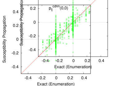
Figure 1: Comparison between the 2-point connected correlation function calculated exactly and that estimated with susceptibility propagation. A 1-in-4 satisfiability instance on a randomly generated factor graph with $N=27$ variables and $M=16$ constraints with Poisson degree distribution with average degree $\overline{\ell}=2.4856$.

IV Numerical investigation of susceptibility propagation in locked occupation models

In this section we study the use of susceptibility propagation, together with decimation, in some locked occupation models. Specifically, we shall study random instances of a locked occupation problem, where the factor graph is uniformly chosen among the graphs with the following degree distribution. All function nodes have degree $K$ and the variables have random degrees chosen from truncated Poisson degree distribution

$$q(\ell)=\begin{cases}0&(\ell=0,1)\\ \frac{\mathrm{e}^{-c}c^{\ell}}{\ell!(1-(1+c)\mathrm{e}^{-c})}.&(\ell\geq 2)\end{cases},$$ (39)

for which the average degree is

$$\overline{\ell}=\sum_{\ell=0}^{\infty}\ell q(\ell)=\frac{c(1-\mathrm{e}^{-c})}{(1-(1+c)\mathrm{e}^{-c})}.$$ (40)

The basic message-passing algorithm that we use is described by the following pseudocode:

Input: Factor graph, constraint-vector, convergence criterion, initial messages

Output: Estimate for 2-point connected correlation functions (or ERROR-NOT-CONVERGED)

• Initialize messages

• Repeat until everything converges

  • Update cavity fields and cavity biases $\nu_{i\rightarrow a}^{(t)}(x_{i})$ and $\hat{\nu}_{a\rightarrow i}^{(t)}(x_{i})$ with (2),(3)

  • Update cavity susceptibilities $\nu_{i\rightarrow a,j}^{(t)}(x_{i},x_{j})$ and $\hat{\nu}_{a\rightarrow i,j}^{(t)}(x_{i},x_{j})$ with (8)(9) with the help of $\nu_{i\rightarrow a}^{(t)}(x_{i})$ and $\hat{\nu}_{a\rightarrow i}^{(t)}(x_{i})$ obtained above

• Compute 1-variable marginals $p_{i}(x_{i})$ from the fixed-point messages $\hat{\nu}_{a\rightarrow i}^{(*)}(x_{i})$ by (4)

• Compute 2-point connected correlation functions $p_{ij}^{\mathrm{conn}}(x_{i},x_{j})$ from the fixed-point messages $\hat{\nu}_{a\rightarrow i}^{(*)}(x_{i})$ and $\hat{\nu}_{a\rightarrow i,a}^{(*)}(x_{i},x_{j})$ by (12)

This algorithm requires a memory proportional to $kMN$, and each step of iteration requires a computation of $\mathcal{O}(N^{2})$ for fixed $k$.

IV.1 Decay of correlations

Fig.2 shows the distribution of magnitude of 2-point connected correlation function computed with susceptibility propagation for all pairs of points in a graph for a fixed distance between the points. One observes a broad dispersion of correlations, and an approximate exponential decay with the distance. Here we measure the distance $d$ with the convention that each edge connecting a variable to a constraint is of length 1.

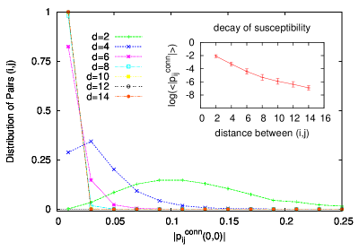
Figure 2: This graph shows how the 2-point connected correlation $p_{ij}^{\mathrm{conn}}(x_{i},x_{j})$ decays as the distance $d$ between $x_{i}$ and $x_{j}$ increases. At each distance $d$, the distribution of $|p_{ij}^{\mathrm{conn}}(0,0)|$ is plotted. In the inset, logarithm of the average of that quantity is plotted against the distance. The instance is 1-in-4 Satisfiability on a random factor graph with $N=1618$ variables and $M=1000$ factors with the truncated Poisson degree distribution with average degree $\overline{\ell}=2.4856$.

Because of this exponential decay, it is possible to use in some cases approximate versions of susceptibility propagation which are faster and use less memory. This is done by truncating to zero the cavity susceptibilities $\nu_{i\rightarrow a,j},\hat{\nu}_{a\rightarrow i,j}$ beyond some prescribed distance $\mathrm{dist}(a,j)>d$ or $\mathrm{dist}(i,j)>d$ and keeping only the correlation functions between pairs of variables not far from each other. Although one can estimate the 2-variable marginal distribution solely from the knowledge of cavity fields (Mézard and Montanari, 2009, Sec.14.2.3),this truncation provides us with a more efficient practical method to compute the 2-variable correlations between variables with $d\geq 4$.

IV.2 Pair Decimation Algorithm

As we mentioned in the introduction, decimation consists in finding a variable with the smallest entropy and fixing it to the most probable value. Assuming that the susceptibility propagation provides us with the good estimate for the 2-point connected correlation, we can think of decimation which acts on a pair of variable instead of a single variable. Let $x_{i}$ and $x_{j}$ be variables. If one defines a random variable $y_{ij}=\mathbf{1}(x_{i}=x_{j})$, one can compute the entropy for $y_{ij}$ once one knows the 2-variable marginal $p_{ij}(x_{i},x_{j})=p_{i}(x_{i})p_{j}(x_{j})+p_{ij}^{\mathrm{conn}}(x_{i},x_{j})$. In pair decimation, one identifies the pair $(i,j)$ with the smallest entropy of $y_{ij}$ and one fixes either $x_{i}=x_{j}$ or $x_{i}+x_{j}=1$, depending on which event is the most probable according to the measured correlation. This results in a reduced smaller CSP, which is still an occupation problem. The efficiency of this novel decimation process depends on whether we can find a pair with less entropy than the single variable with the smallest entropy. It is easy to see that, in the absence of correlations, namely if $p_{ij}(x_{i},x_{j})=p_{i}(x_{i})p_{j}(x_{j})$, then the entropy of $y_{ij}$ is larger than the one of $x_{i}$ or $x_{j}$. So the whole procedure relies on being able to detect correlations. Fig.3 shows that strongly correlated pairs can be found.

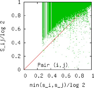
Figure 3: Comparison between the minimum entropy $\min(S_{i},S_{j})$ (where $S_{i}$ and $S_{j}$ are the entropies of $x_{i}$, $x_{j}$ )and $S_{ij}$, that of $y_{ij}=\mathbf{1}(x_{i}=x_{j})$. The instance is 1-in-4 Satisfiability on a random factor graph with $N=1618$ variables and $M=1000$ factors with the truncated Poisson degree distribution with average degree $\overline{\ell}=2.4856$.

In practice, we have used the following decimation algorithm which mixes the two strategies of single-variable decimation and pair decimation:

Input: Factor graph, constraint-vector, convergence criterion, initial messages

Output: A satisfying assignment (or FAIL-NOT-FOUND)

• While graph has more than $R$ variables:

  • Compute local entropy estimates for the 1-variable marginals

  • Compute local entropy estimates for the 2-variable marginals

  • if ‘heuristic criterion finds that single-variable decimation is better’,

    • then fix the value of the variable.

    • else identify a variable in the pair with the other (or its negation)

  • Locate completely locked nearest neighbor pairs

  • Clean the graph

    • Fix the value of isolated variables

  • Do warning propagation.

  • Identify local locked pairs

• When the number of variables is equal to or smaller than $R$: perform an exhaustive search for satisfying assignments. If found

  • Then return the satisfying assignment

  • Else return FAIL-NOT-FOUND

The heuristic criterion that we use in order to decide between the two types of decimation is the following. We locate a variable with the least entropy and a pair of variables with the least entropy for $y_{ij}$. When the former is less than $S_{\mathrm{th}}$ or is smaller than the latter, we choose to do single-variable decimation.

For the optimal reduction of the entropy within a decimation step, it is reasonable to set $S_{\mathrm{th}}=0$. However, we find that $S_{\mathrm{th}}>0$ performs better for finding a satisfying assignment. The optimal value of $S_{\mathrm{th}}$ depends on the type of locked occupation model and the average degree. This fact can be interpreted as follows: the estimation of 1-variable marginals is more precise than the 2-variable ones within given computational resource, thus it is advantageous to respect the former if it is decisively small.

Warning propagation is a message-passing algorithm described in Mézard et al. (2003); Montanari et al. (2007). It logically infers the value of variables one by one from local structure of the factor graph.

In the identification of local locked pairs, we look at each degree-2 constraint and see if the constraint enforces $y_{ij}=0$ or $y_{ij}=1$. If it is the case, we identify this pair.

The threshold for exhaustive search has been fixed in our simulations to $R=16$.

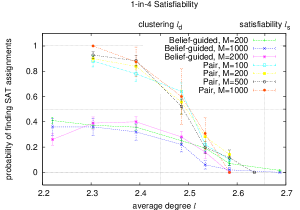
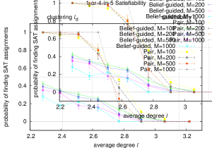
Figure 4: Success probability of pair decimation process for 1-in-4 satisfiability $A=(0,1,0,0,0)$ (left) and 1-or-4-in-5 satisfiability $A=(0,1,0,0,1,0)$ (right) on a random factor graph with $M$ constraints and average degree $\overline{\ell}$ (right), plotted versus $\overline{\ell}$ . For comparison, the performance of simple belief-guided decimation process is shown. The vertical lines show the clustering and satisfiability thresholds.

The performance of this algorithm is shown for 1-in-4 satisfiability $A=(0,1,0,0,0)$ and 1-or-4-in-5 satisfiability $A=(0,1,0,0,1,0)$ in Fig.4. For 1-in-4 satisfiability, data with randomization is presented: instead of fixing the most polarized variable or pair, we fix a variable or pair randomly chosen among a fixed number (here we adopt 8) of most polarized variables/pairs. The figure also shows the two important thresholds for these problems, which are values of the average degree (a measure of the number of constraints) separating qualitatively distinct phases. The probability that a satisfying assignment exists drops from 1 to 0 at the ‘satisfiability threshold’ $\ell_{s}$ in the large factor graph limit. Between the ‘clustering threshold’ (Zdeborová and Mézard (2008) and the satisfiability threshold, although the satisfying assignments still exist with probability one, it is very difficult to find one by the algorithms known so far, because of the splitting of the set of solutions into clusters. In both LOPs the performance is improved compared to the simple belief-guided decimation employed in Zdeborová and Mézard (2008). Especially for 1-or-4-in-5, the present algorithm works well above the clustering threshold, a region of $\overline{\ell}$ where all known algorithms are reported to perform poorly Zdeborová and Mézard (2008).

V Conclusion and Discussion

We have shown how to find satisfying assignments for locked occupation problems based on the measurement of correlation among variables. This is in contrast with the conventional method which is guided by 1-variable marginals only. Since flipping a variable in a LOP forces another variable far apart to be flipped, the performance of the algorithm is improved when we take the correlations into account.

We have calculated correlations with the susceptibility propagation. In this method, the correlations between variables which ar efar apart can be calculated as well as between those which are neighbors. Namely, the convergence property is controlled by a single matrix $\mathcal{M}$.

The susceptibility propagation, however, requires more computational time and memory resource than the simple belief propagation. Therefore, as the problem becomes larger, we face a (polynomial) increase of computation time. The truncation introduced in subsectionIV.1 might give a remedy since it reduces by a factor of $N$ the computation time as well as the memory use. The decay of correlation suggests that this is a reasonable approximation. We have performed preliminary experiments to find the performance of this approximate algorithm. As expected, it behaves similarly to that without truncation, the performance being only slightly degraded.

References

- Mézard and Zecchina (2002) M. Mézard and R. Zecchina, Physical Review E 66, 56126 (2002).
- Krzakala et al. (2007) F. Krzakala, A. Montanari, F. Ricci-Tersenghi, G. Semerjian, and L. Zdeborová, Proceedings of the National Academy of Sciences 104, 10318 (2007).
- Chavas et al. (2005) J. Chavas, C. Furtlehner, M. Mézard, and R. Zecchina, Journal of Statistical Mechanics 11016 (2005).
- Mézard and Mora (2008) M. Mézard and T. Mora (2008), arXiv:0803.3061.
- Mézard et al. (2002) M. Mézard, G. Parisi, and R. Zecchina, Science 297, 812 (2002).
- Zdeborová and Mézard (2008) L. Zdeborová and M. Mézard, Physical Review Letters 101, 078702 (2008).
- Zdeborová and Mézard (2008) L. Zdeborová and M. Mézard, Journal of Statistical Mechanics p. P12004 (2008).
- Mézard et al. (2003) M. Mézard, F. Ricci-Tersenghi, and R. Zecchina, Journal of Statistical Physics 111, 505 (2003).
- Montanari and Rizzo (2005) A. Montanari and T. Rizzo, Journal of Statistical Mechanics: Theory and Experiment 10, P10011 (2005).
- Chertkov and Chernyak (2006) M. Chertkov and V. Chernyak, Physical Review E 73, 065102 (2006).
- Parisi and Slanina (2006) G. Parisi and F. Slanina, Journal of Statistical Mechanics 602 (2006).
- Zdeborová (2008) L. Zdeborová, Ph.D. thesis, Université Paris-Sud (2008), arxiv:0806.4112.
- Raymond et al. (2007) J. Raymond, A. Sportiello, and L. Zdeborová, Physical Review E 76, 11101 (2007).
- Gallager (1962) R. Gallager, Information Theory, IEEE Transactions on 8, 21 (1962).
- Kschischang et al. (2001) F. Kschischang, B. Frey, and H. Loeliger, IEEE Transactions on Information Theory 47, 498 (2001).
- Yedidia et al. (2003) J. Yedidia, W. Freeman, and Y. Weiss, Understanding belief propagation and its generalizations (Science & Technology Books, 2003), pp. 239–236.
- Mézard and Montanari (2009) M. Mézard and A. Montanari, Information, Physics and Computation (Oxford University Press, 2009).
- Mora (2007) T. Mora, Ph.D. thesis, Université Paris-Sud (2007), http://tel.archives-ouvertes.fr/tel-00175221/en/.
- Creignou and Daude (1999) N. Creignou and H. Daude, Discrete Applied Mathematics 96, 41 (1999).
- Montanari et al. (2007) A. Montanari, F. Ricci-Tersenghi, and G. Semerjian (2007), arXiv:0709.1667.