Projection operator approach to lifetimes of electrons in metals

Abstract

We present an alternative approach to the calculation of the lifetime of a single excited electron (hole) which interacts with the Fermi sea of electrons in a metal. The metal is modelled on the level of a Hamilton operator comprising a pertinent dispersion relation and scattering term. To determine the full relaxation dynamics we employ an adequate implementation of the time-convolutionless projection operator method (TCL). This yields an analytic expression for the decay rate which allows for an intuitive interpretation in terms of scattering events. It may furthermore be efficiently evaluated by means of a Monte-Carlo integration scheme. As an example we investigate aluminium using, just for simplicity, a jellium-type model. This way we obtain data which are directly comparable to results from a self-energy formalism. Our approach applies to arbitrary temperatures.

I Introduction

For several decades, the dynamics of excited electrons in metals has been the subject of intense research in theoretical and experimental solid state physics. Quinn1 ; Quinn2 ; baym ; Bauer1 ; Bauer4 ; Bauer2 ; Echenique1 ; Echenique2 ; Hofer ; Jaeckle . These investigations are motivated by the fact that a lot of physical and chemical properties of metallic materials depend essentially on those dynamics Pines ; Mahan ; Kittel . Lifetimes of (photo)excited electrons in metals are always short (on the order of femtoseconds) but the immense progress in ultrafast laser technology now allows for an experimental determination of such times, corresponding investigations are ongoing Bauer3 .

Today a number of methods are used to calculate lifetimes of electrons. Practically all of them are formulated within the framework of Green’s functions (many-body theory) and aim at determining the self-energy, particularly its imaginary part Fetter ; Kirzhnits ; Brown . Many of them employ a screened interaction (“W”) and a truncated expansion of the self energy in terms of this screened interaction (“GW-approximation”) Hedin1 ; Hedin2 ; Echenique1 ; Echenique2 ; Chulkov1 ; Chulkov2 ; Rubio ; Schoene ; Rolli1 ; Rolli2 ; Mari ; Nechaev . The screened interaction is frequently obtained through a “random phase approximation” (RPA) Pines . For a simple, sufficiently dense, homogeneous gas of electrons interacting through coulomb repulsion (jellium model) an approach along the above scheme is even feasible analytically and yields a closed expression for the lifetimes close to the Fermi edge (see below) Quinn1 ; Quinn2 . In a certain sense (which is described in more detail below (LABEL:HamJel)) this approach leads to lifetimes which may quantitatively be compared to experimental data on e.g., aluminium Bauer1 ; Schoene ; Nechaev . Of course timely state of the art approaches go beyond jellium and exploit not only the traditional self-energy formalism but also density functional methods, etc. Schoene ; Rolli1 ; Rolli2 ; Mari .
Our approach is, in contrary, not based on Green’s functions at all but on projection operator techniques. A main motivation of our work is to demonstrate that a pertinent projective approach Nakajima ; Zwanzig ; Grabert ; Fulde ; Rau ; Burnett ; Neu ; Breuer is also capable to produce quantitative results on lifetimes. Our central formula from which the lifetimes are eventually calculated is in accord with expressions that may be derived within the above many-body approach (see below (LABEL:final)). Furthermore it allows for an interpretation in terms of scattering events. This encourages a further development of projection techniques as alternative quantitative tools for the investigation of relaxation and transport dynamics in condensed matter systems (find more on this at the end of Sec. IV). However, our approach starts form an effective model comprising pertinent quasi-particle dispersion relations and an appropriate screened interaction. The (generically subtle) provision of such a suitable effective model is not part of our present analysis, the effective model thus has to be supplied by other means.
The article at hand is organized as follows: In Sec. II we give a very brief introduction to the time-convolutionless projection operator method Breuer and apply it to a general interacting quantum gas thus obtaining an expression for the electronic lifetime. In Sec. III we evaluate this expression numerically for a “screened” jellium model tuned to describe aluminium. We compare our results to other available data and comment on computing times. Eventually we close with discussion, summary and outlook.

II projective approach to occupation number dynamics in interacting quantum gases

To determine the lifetime of an electron initially occupying some momentum eigenstate we analyze the dynamics of the corresponding occupation number. A formalism which allows for such an analysis is the TCL-method Breuer . In general the latter is a perturbative projection operator technique which produces autonomous equations of motion for the variables of interest (“relevant information”). The technique may be applied to quantum system with a Hamiltonian of the type $\hat{H}=\hat{H}_{0}+\lambda\hat{V}$ where $\lambda$ has to be in some sense small Breuer In order to apply this method one first has to construct a suitable projection operator $\mathcal{P}$. Formally, this is a linear map which projects any density matrix $\varrho(t)$ to a matrix $\mathcal{P}\varrho(t)$ that is determined by a certain set of variables. These variables should match with the variables of interest. Moreover $\mathcal{P}$ has to fulfill the property of a projection operator, that is $\mathcal{P}^{2}=\mathcal{P}$. For initial states with $\mathcal{P}\varrho(0)=\varrho(0)$ the TCL scheme leads to a time-local differential equation for the dynamics of $\mathcal{P}\varrho$:

$$\partial_{t}\mathcal{P}\varrho(t)=\Gamma(t)\mathcal{P}\varrho(t),\hskip 14.22636pt\Gamma(t)=\sum\limits_{k=1}^{\infty}\lambda^{k}\Gamma_{k}(t),$$ (1)

where the perturbative expansion used in the last equations is in principle exact. However, for a description to leading order, which is typically and in our case the second order, one has to determine $\Gamma_{2}(t)$. Whether or not a leading order description will yield a reasonable result is a somewhat subtle question Christian but the expansion is well controlled and systematic, i.e, in principle higher order terms could be incorporated in a straightforward manner Breuer . A widely accepted indicator for the validity of the truncation is a clear timescale separation between the resulting relaxation dynamics and the decay of the correlation function, the latter being introduced below. However, here we are going to focus on the leading order and comment on the timescales below when we eventually arrive at concrete lifetimes. In the literature Breuer one finds

$$\Gamma_{2}(t)=\int\limits_{0}^{t}dt^{\prime}\mathcal{P}\mathcal{L}(t)\mathcal{L}(t^{\prime})\mathcal{P},$$ (2)

with $\mathcal{L}(t)=\frac{\imath}{\hbar}[\hat{V}(t),\#]$, where $\#$ denotes a placeholder for an operator which shall be inserted into the commutator. $V(t)$ refers to a perturbation in the interaction picture. With (1) and (2) we obtain:

$$\partial_{t}\mathcal{P}\varrho(t)=\int\limits_{0}^{t}dt^{\prime}\mathcal{P}\mathcal{L}(t)\mathcal{L}(t^{\prime})\mathcal{P}\varrho(t).$$ (3)

Now for an concrete application we have to specify the underlying quantum model and a suitable projection operator.
The systems we investigate are interacting quantum gases, here of the “spinless fermions”- type. The corresponding Hamiltonians may be written as

$$\underbrace{\sum\limits_{{\bf k}}\varepsilon_{{\bf k}}a_{{\bf k}}^{\dagger}a_{{\bf k}}}_{\hat{H}_{0}}+\underbrace{\frac{1}{2}\sum\limits_{{\bf k},{\bf l},{\bf q}}V({\bf q})a_{{\bf k+q}}^{\dagger}a_{{\bf l-q}}^{\dagger}a_{{\bf l}}a_{{\bf k}}}_{\hat{V}},$$ (4)

where $\varepsilon_{{\bf k}}$ denotes a dispersion relation of free particles and $V({\bf q})$ the matrix elements of an interaction which depends on the concrete system. This Hamiltonian is of the above mentioned form as long as the interaction term $\hat{V}$ is in adequate sense “small” (see below). As will be demonstrated below (cf. Sec. III) it is thus reasonable to choose for $\varepsilon_{{\bf k}}$ pertinent quasi-particle dispersion relations and particularly for $V({\bf q})$ an adequate screened interaction. Note that we neglect the spin quantum number since the system we consider in this work is paramagnetic and without any magnetic fields the dispersion relation is the same for both spin channels. Below we are going to take care of this “spin degeneracy” in a very simple form (cf. text following (18). For the non-interacting many-particle system we may directly write down the wavenumber (momentum) dependent “single particle equilibrium density operator” as:

$$\varrho_{{\bf j}}^{eq}:=f_{{\bf j}}(\mu,T)a_{\bf j}^{\dagger}a_{\bf j}+(1-f_{{\bf j}}(\mu,T))a_{\bf j}a_{\bf j}^{\dagger},$$ (5)

with $f_{{\bf j}}(\mu,T)=(\exp((\varepsilon({\bf j})-\mu)/k_{B}T)+1)^{-1}$ being the Fermi distribution. Since we are interested in temperature regimes close to $T=0$K but still $T\neq 0$K we can set the chemical potential $\mu$ $\approx$ $\varepsilon_{F}$. Further we abbreviate $f_{{\bf j}}(\varepsilon_{F},T)$ as $f_{{\bf j}}$. The equilibrium density operator, again for the non-interacting case, of the total system, $\varrho^{eq}$, may be written as the tensor product of the single particle density operators, i.e.

$$\varrho^{eq}:=\bigotimes\limits_{{\bf i}}\varrho_{{\bf i}}^{eq},\qquad\text{note also}\qquad\tilde{\varrho}:=\bigotimes\limits_{{\bf i}\neq{\bf j}}\varrho_{{\bf i}}^{eq}.$$ (6)

Here, for later reference, $\tilde{\varrho}$ denotes the total density operator of the system which does not contain the subspace with respect to the momentum mode ${\bf j}$, i.e. it is $\varrho^{eq}=\tilde{\varrho}\otimes\varrho_{{\bf j}}^{eq}$. We should, also for later reference, mention here that while $\varrho^{eq}$ is strictly speaking just the equilibrium state of the non-interacting system, it is routinely considered to describe the single particle properties of the weakly interacting system more or less correctly. Thus, if single particle observables relax towards equilibrium due to the interactions (scattering), we expect them to relax towards values corresponding to $\varrho^{eq}$.
For the investigations of the dynamics of excited states we define an operator $\Delta_{{\bf j}}$ (for the remainder of this paper $|{\bf j}\rangle$ denotes the excited state) as

$$\Delta_{{\bf j}}:=(1-f_{{\bf j}})a_{\bf j}^{\dagger}a_{\bf j}-f_{{\bf j}}a_{\bf j}a_{\bf j}^{\dagger}=a_{\bf j}^{\dagger}a_{\bf j}-f_{{\bf j}},$$ (7)

which describes the deviation of the mode occupation number $n_{\bf j}=a_{\bf j}^{\dagger}a_{\bf j}$ from its thermal equilibrium. Now, in order to apply the TCL method to this model we construct a suitable projector as follows:

$$\mathcal{P}\varrho(t)=\varrho^{eq}+\frac{1}{\sigma^{2}_{{\bf j}}}\text{Tr}\{\Delta_{{\bf j}}\varrho(t)\}\tilde{\varrho}\otimes\Delta_{{\bf j}},$$ (8)

with $\varrho(t)$ being the density operator which describes the actual state of the system, $d_{{\bf j}}(t):=$Tr$\{\Delta_{{\bf j}}\varrho(t)\}$ denotes the time dependent expectationvalue of $\Delta_{{\bf j}}$ and $\sigma^{2}_{{\bf j}}:=(1-f_{{\bf j}})^{2}+f_{{\bf j}}^{2}=$Tr$\{\Delta_{{\bf j}}^{2}\}$. It is straightforward to show that with the above definitions $\mathcal{P}$ is a projector and fulfills $\mathcal{P}^{2}\varrho(t)=\mathcal{P}\varrho(t)$. Note that Tr$\{\varrho^{eq}\Delta_{{\bf j}}\}=0$ and Tr$\{\Delta_{{\bf j}}\tilde{\varrho}\otimes\Delta_{{\bf j}}\}=\sigma^{2}_{{\bf j}}$. Before we eventually concretely apply (3) to our model we make the following approximation for an expression that appears in the computation of (3):

$$\mathcal{L}(t^{\prime})\mathcal{P}\varrho(t) = \frac{\imath}{\hbar}[\hat{V}(t^{\prime}),\varrho^{eq}]+\frac{\imath}{\hbar}[\hat{V}(t^{\prime}),\tilde{\varrho}\otimes\Delta_{{\bf j}}]\frac{d_{{\bf j}}(t)}{\sigma^{2}_{{\bf j}}}$$ (9)

$$\approx \frac{\imath}{\hbar}[\hat{V}(t^{\prime}),\tilde{\varrho}\otimes\Delta_{{\bf j}}]\frac{d_{{\bf j}}(t)}{\sigma^{2}_{{\bf j}}},$$

The neglected commutator term essentially describes the dynamics of the equilibrium state of the non-interacting system. Eventually we are interested in a single particle observable. As already mentioned above, the equilibrium state of the non-interacting system is believed to reasonably describe single particle observables in equilibrium even for weakly interacting systems. Since an equilibrium state is constant, the above commutator should not significantly contribute to the relevant dynamics, thus we drop it. Keeping the term and performing all following steps yields eventually an expression which can explicitly shown to be indeed negligible in the weak coupling limit. For clarity and briefness we omit this calculation here.
If we apply now (3) to (8) and make use of (9) we obtain

$$\partial_{t}\mathcal{P}\varrho(t)=\frac{1}{\sigma^{2}_{{\bf j}}}\partial_{t}d_{{\bf j}}(t)\cdot\tilde{\varrho}\otimes\Delta_{{\bf j}}=\int\limits_{0}^{t}dt^{\prime}\varrho^{eq}$$

$$- \int\limits_{0}^{t}dt^{\prime}\frac{1}{\sigma^{4}_{{\bf j}}\hbar^{2}}\text{Tr}\{[\Delta_{{\bf j}}[\hat{V}(t),[\hat{V}(t^{\prime}),\tilde{\varrho}\otimes\Delta_{{\bf j}}]]\}\tilde{\varrho}\otimes\Delta_{{\bf j}}d_{{\bf j}}(t).$$

Multiplying both sides of (LABEL:equ2) with $\Delta_{{\bf j}}$ and taking the trace leads to:

$$\partial_{t}d_{{\bf j}}(t)=-\underbrace{\frac{1}{\hbar^{2}\sigma^{2}_{{\bf j}}}\int\limits_{0}^{t}dt^{\prime}\text{Tr}\{[\Delta_{{\bf j}}[\hat{V}(t),[\hat{V}(t^{\prime}),\tilde{\varrho}\otimes\Delta_{{\bf j}}]]\}}_{\Gamma_{\bf j}(t)}d_{{\bf j}}(t),$$

(11)

where $\Gamma_{\bf j}(t)$ appears as a time-dependent damping rate of the mode ${\bf j}$. If $\Gamma_{\bf j}(t)$ turns out to be approximately time-independent, the usual exponential relaxation results. With the substitution $t^{\prime}=t-\tau$ and exploiting $[\tilde{\varrho}\otimes\Delta_{{\bf j}},\hat{H}_{0}]=[\Delta_{{\bf j}},\hat{H}_{0}]=0$ as well as some trace properties, we obtain for the rate:

$$\Gamma_{\bf j}(t)=\frac{1}{\hbar^{2}\sigma^{2}_{{\bf j}}}\int\limits_{0}^{-t}d\tau\underbrace{\text{Tr}\{[\hat{V}(\tau),\tilde{\varrho}\otimes\Delta_{{\bf j}}]\cdot[\hat{V}(0),\Delta_{{\bf j}}]\}}_{C(\tau)},$$ (12)

where $C(\tau)$ denotes the correlation function which is real due to the fact that both commutators are hermitian. The concrete evaluation of this expression with respect to our model is straightforward but somewhat lengthy. Thus the full computation is given in the Appendix, here we only give and discuss the results After exploiting the commutators within the trace we finally obtain for the rate:

$$\Gamma_{\bf j}(t,T) = \frac{1}{\tau_{{\bf j}}}=-\frac{2}{\hbar^{2}\sigma^{2}_{{\bf j}}}\sum\limits_{{\bf k},{\bf q}}\int\limits_{0}^{-t}d\tau|V({\bf q})|^{2}F({\bf k},{\bf q},{\bf j},T)$$

$$\times \cos\left((\omega_{{\bf k}+{\bf q}}+\omega_{{\bf j}-{\bf q}}-\omega_{{\bf k}}-\omega_{{\bf j}})\tau\right)$$

$$= \frac{2}{\hbar^{2}\sigma^{2}_{{\bf j}}}\sum\limits_{{\bf k},{\bf q}}|V({\bf q})|^{2}F({\bf k},{\bf q},{\bf j},T)\cdot t\cdot\text{sinc}\left(\omega({\bf k},{\bf q},{\bf j})t\right),$$

with:

$$\omega({\bf k},{\bf q},{\bf j}) := \omega_{{\bf k}+{\bf q}}+\omega_{{\bf j}-{\bf q}}-\omega_{{\bf k}}-\omega_{{\bf j}},$$

$$F({\bf k},{\bf q},{\bf j},T) := \underbrace{(1-f_{{\bf j}})(1-f_{{\bf j-q}})(1-f_{{\bf k+q}})f_{{\bf k}}}_{F_{1}({\bf k},{\bf q},{\bf j},T)}$$

$$+ \underbrace{f_{{\bf j}}f_{{\bf j-q}}f_{{\bf k+q}}(1-f_{{\bf k}})}_{F_{2}({\bf k},{\bf q},{\bf j},T)}$$

and sinc$(\omega t)$ denotes the sinus cardinalis. Obviously the integral $\int_{-\infty}^{+\infty}t\cdot$sinc$(\omega t)d\omega$ is independent of $t$. Furthermore the function gets more and more peaked with increasing $t$ such that, as wellknown,

$$\lim_{t\rightarrow\infty}\frac{\sin(\omega t)}{\omega}=\pi\delta(\omega).$$ (15)

Hence, since dispersion relations are smooth functions of the wavenumber, we expect the rate $\Gamma_{\bf j}(t,T)$ to become indeed time-independent for times larger than $\tau_{c}$, if $1/\tau_{c}$ is an energyscale on which dispersion relations may be linearized. Thus for times $t$ larger than $\tau_{c}$ we may with good precision approximate (here we neglect the factor $\sigma^{-2}_{{\bf j}}$ since for temperatures $T\approx 0$K it is $\sigma^{-2}_{{\bf j}}\approx 1$):

$$\Gamma_{\bf j}(T) =\frac{1}{\tau_{{\bf j}}}=\frac{2\pi}{\hbar}\sum\limits_{{\bf k},{\bf q}}|V({\bf q})|^{2}\delta\left(\varepsilon_{{\bf k}+{\bf q}}+\varepsilon_{{\bf j}-{\bf q}}-\varepsilon_{{\bf k}}-\varepsilon_{{\bf j}}\right)$$

$$\times \{(1-f_{{\bf j}})(1-f_{{\bf j-q}})(1-f_{{\bf k+q}})f_{{\bf k}}+f_{{\bf j}}f_{{\bf j-q}}f_{{\bf k+q}}(1-f_{{\bf k}})\}.$$

This expression is one of our main results. In principle it allows for a direct calculation of lifetimes for any fermionic system with given quasi-particle dispersion relations and screened scattering term. Very similar formulas can be found in textbooks in the context of transport and relaxation, see, e.g., Jaeckle ; Pines . They are often derived on the basis of an ad hoc application of Fermi’s golden rule. A closer look reveals that such an expression can also be obtained from an analysis along the lines described in the introduction (”RPA-GW”) by using the static-limit form of the screened interaction. Since our further quantitative determination only consists in a numerical evaluation of (LABEL:final) the outcome is equivalent to the one obtained by the above treatment. And since, as outlined in the following, (LABEL:final) is in accord with a standard scattering interpretation, obviously both, the projective and the above version of the many-body approach amount more or less to the counting of scattering events.
The contributions to the decay rate corresponding to $F_{1}$ and $F_{2}$ allow for an intuitive interpretation, at least for low temperatures.
$F_{1}$: This term accounts for the decay of an electron from a momentum mode ${\bf j}$ above the Fermi sea, cf. Fig. (1a). Due to the factor $(1-f_{{\bf j}})$ it only significantly contributes to the occupation number dynamics of such modes that are unoccupied in equilibrium. Those occupation numbers may only deviate from equilibrium towards an excess of electrons. According to the other three factors only those summands contribute that correspond to the electron at ${\bf j}$ colliding with an electron from within the Fermi sea ${\bf k}$, such that the post-collision momenta ${\bf k+q}$, ${\bf j-q}$ lay in the unoccupied region above the Fermi sea.
$F_{2}$: This term accounts for the decay of a hole from a momentum mode ${\bf j}$ within the Fermi sea, cf. Fig. (1b). Due to the factor $f_{{\bf j}}$ it only significantly contributes to the occupation number dynamics of such modes that are occupied in equilibrium. Those occupation numbers may only deviate from equilibrium towards a shortage of electrons, i.e., holes. According to the other three factors only those summands contribute that correspond to two electrons from within the Fermi sea ${\bf k+q}$, ${\bf j-q}$ colliding such that one post-collision momentum ${\bf k}$ lays in the unoccupied region above the Fermi sea and the other lays exactly at ${\bf j}$ such as to fill up the hole.

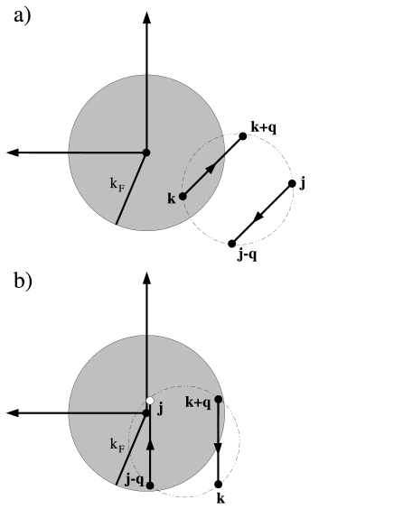
Figure 1: Schematic representation of the underlying collision processes in momentum space as described in the text ($k_{F}$ denotes the Fermi momentum).
a) A collision process through which an excited electron at momentum ${\bf j}$ vanishes from its initial momentum mode.
b) A collision process ”filling” a hole within the Fermi sphere at ${\bf j}$.
The dashed circles denote the possible outgoing momenta under momentum and energy conservation.

III Application to a jellium model with screened interaction

In this section we now apply our result for the decay rates to a jellium modell featuring a Thomas-Fermi screened interaction. The latter will eventually be tuned to correspond to aluminium. However, to repeat, the main intention of this work is not to calculate decay rates in aluminium with extreme precision, but to concretely demonstrate the feasibility of our method. The Hamiltonian of the model is given by:

$$\hat{H}_{J} = \frac{\hbar^{2}}{2m_{e}}\sum\limits_{{\bf k}}k^{2}a_{{\bf k}}^{\dagger}a_{{\bf k}}$$

$$+ \frac{1}{2}\sum\limits_{{\bf k,l,q}}\frac{e^{2}}{\Omega\varepsilon_{0}({\bf q}^{2}+{\bf q}^{2}_{TF})}a_{{\bf k+q}}^{\dagger}a_{{\bf l-q}}^{\dagger}a_{{\bf l}}a_{{\bf k}},$$

where $\Omega$ denotes the volume of the solid and ${\bf q}_{TF}$ the so called Thomas-Fermi wavenumber which is related to the Fermi wavevector and the Wigner-Seitz radius by $(q_{TF}/k_{F})^{2}=0.665r_{S}$ (with $r_{S}=(\frac{3}{4\pi\rho_{0}})^{\frac{1}{3}}\frac{1}{a_{0}}$, $a_{0}$ being the Bohr radius, $\varepsilon_{F}=(9\pi/4)^{\frac{2}{3}}\frac{1}{r_{S}^{2}}$[ryd], $k_{F}=(9\pi/4)^{\frac{1}{3}}\frac{1}{a_{0}r_{S}}$, $q_{TF}=(12/\pi)^{\frac{1}{3}}\frac{1}{a_{0}\sqrt{r_{S}}}$). Note that our model only comprises electrons, no phonons. Thus the result on the decay rate has to be compared to that part of the total decay rate that stems from electron-electron scattering only. In real aluminium there is evidence that the total lifetime is also significantly shortened due to electron-phonon scattering Bauer1 ; Nechaev . We apply now (LABEL:final) to this model which yields:

$$\Gamma_{\bf j}(T) = \frac{1}{\tau_{{\bf j}}}=\frac{4\pi}{\hbar}\sum\limits_{{\bf k},{\bf q}}\left(\frac{e^{2}}{\Omega\varepsilon_{0}({\bf q}^{2}+{\bf q}_{TF}^{2})}\right)^{2}F({\bf k},{\bf q},{\bf j},T)$$ (18)

$$\times \delta\left(\varepsilon_{{\bf k}+{\bf q}}+\varepsilon_{{\bf j}-{\bf q}}-\varepsilon_{{\bf k}}-\varepsilon_{{\bf j}}\right)$$

where the auxiliary factor 2 arises from the fact that for each ${\bf k}$ we have two one-electron states (one for each spin) which is taken into account by this additional factor. If we now replace the sums in (18) by integrals by the rule $\sum\limits_{{\bf k}}f({\bf k})\rightarrow(2\pi)^{-3}\Omega\int d{\bf k}f({\bf k})$ we obtain for $\Gamma_{\bf j}(T)$:

$$\Gamma_{\bf j}(T) = \frac{4\Omega^{2}}{2^{6}\hbar\pi^{5}}\iint d{\bf k}d{\bf q}\left(\frac{e^{2}}{\Omega\varepsilon_{0}({\bf q}^{2}+{\bf q}_{TF}^{2})}\right)^{2}F({\bf k},{\bf q},{\bf j},T)$$

$$\times \delta\left(\varepsilon_{{\bf k}+{\bf q}}+\varepsilon_{{\bf j}-{\bf q}}-\varepsilon_{{\bf k}}-\varepsilon_{{\bf j}}\right)$$

$$= \frac{e^{4}}{16\hbar\varepsilon_{0}^{2}\pi^{5}}\iint d{\bf k}d{\bf q}\frac{F({\bf k},{\bf q},{\bf j},T)}{({\bf q}^{2}+{\bf q}_{TF}^{2})^{2}}$$

$$\times \delta\left(\varepsilon_{{\bf k}+{\bf q}}+\varepsilon_{{\bf j}-{\bf q}}-\varepsilon_{{\bf k}}-\varepsilon_{{\bf j}}\right).$$

For the numerical calculation it is advantageous to transform the momenta to dimensionless parameter thus we introduce coordinates relative to the Fermi momentum: ${\bf k}\rightarrow k_{F}\cdot{\bf k^{\prime}}$, thus ${\bf q}\rightarrow k_{F}\cdot{\bf q^{\prime}}$ and thus ${\bf j}\rightarrow k_{F}\cdot{\bf j^{\prime}}$.

Figure 2: Comparison of the lifetimes of excited electrons in aluminium as arising from electron-electron scattering only. Displayed is the regime close to the Fermi edge. The open triangles correspond to data obtained from from the approach at hand, i.e., integration of (LABEL:FinalRate) (T$=10$K). The solid circles are experimental data corrected for transport effects taken from (Bauer1 ) while the solid line is the analytical result from Quinn1 . Solid diamonds are the results of an DFT-GW calculation as shown in Echenique2 . The number of sample points for the Monte-Carlo integration of (LABEL:FinalRate) is N=$2\cdot 10^{7}$, the broadening parameter is $\sigma$=1/25.

Applying all these substitutions to (LABEL:Rate2) leads to:

$$\Gamma_{{\bf j}^{\prime}}(T) = \frac{m_{e}e^{4}}{8\hbar^{3}\varepsilon_{0}^{2}\pi^{5}}\iint d{\bf k}^{\prime}d{\bf q}^{\prime}\frac{F({\bf k}^{\prime},{\bf q}^{\prime},{\bf j}^{\prime},T)}{({\bf q}^{\prime 2}+0.665r_{S})^{2}}$$ (20)

$$\times \delta(({\bf k}^{\prime}+{\bf q}^{\prime})^{2}+({\bf j}^{\prime}-{\bf q}^{\prime})^{2}-{\bf k}^{\prime 2}-{\bf j}^{\prime 2}),$$

with $f_{{\bf k}^{\prime}}=(\exp\left(\beta\varepsilon_{F}({\bf k}^{\prime 2}-1)\right)+1)^{-1}$ and $m_{e}=9.1\cdot 10^{-31}$kg the free electron mass.
For the numerical evaluation of the last expression we approximate the delta distribution by a suitable non-singular, e.g., Gaussian-type function:

$$\delta_{\sigma}(\omega)\approx\frac{1}{\sigma\sqrt{2\pi}}e^{-\frac{\omega^{2}}{2\sigma^{2}}},$$ (21)

where $\sigma$ denotes the standard deviation which has to be in some sense small. More details on this somewhat subtle approximation are given below. Thus we get the following integral for the rate:

$$\Gamma_{{\bf j}^{\prime}}(T) = \frac{1.05\text{fs}^{-1}}{\sigma}\cdot\iint d{\bf k}^{\prime}d{\bf q}^{\prime}\frac{F({\bf k}^{\prime},{\bf q}^{\prime},{\bf j}^{\prime},T)}{({\bf q}^{\prime 2}+0.665r_{S})^{2}}$$

$$\times \exp\left(\frac{1}{2\sigma^{2}}\left(({\bf k}^{\prime}+{\bf q}^{\prime})^{2}+({\bf j}^{\prime}-{\bf q}^{\prime})^{2}-{\bf k}^{\prime 2}-{\bf j}^{\prime 2}\right)^{2}\right).$$

For aluminium we choose $r_{S}=2.07$. The six dimensional integrals are solved numerically without any further simplification using a standard Monte-Carlo package as implemented in the Mathematica code. Of course this specific integral could be evaluated in other ways, however, to demonstrate the feasibility of our approach in general we proceed as indicated.
As one can see in Fig. 2 there is rather good agreement between our results, other theoretical approaches and experiment. Our data is denoted by open triangles. The solid line corresponds to the many-body approach based on jellium Quinn1 as outlined in the introduction. The solid diamonds denote the result of a more sophisticated many-body approach which takes the lattice into account and exploits density functional theory Echenique2 . The solid circles indicate the parts of the measured decay rates that are attributed to direct electron-electron scattering, i. e., after removal of transport effects according to Bauer1 . Fig.3 shows the analytic result from Quinn1 ($263r_{S}^{-5/2}(\varepsilon-\varepsilon_{F})^{-2}[\text{eV}]^{2}[\text{fs}]$), which is supposed to be valid close to the Fermi edge, boldly continued to all energies (solid line). Furthermore results of our approach for all energies are displayed (dots). Obviously there are deviations for electrons at higher energies while the agreement remains very good in the limit of “low-energy holes” .
However, a comment should be added here. For this more or less realistic model we get lifetimes on the order of some femtoseconds. The decaytime of the correlation function (12) is, very roughly, on the order of $h/\epsilon_{max}$, with $\epsilon_{max}$ being the bandwith. For about 10eV this yields ca. half a femtosecond. Thus the separation of those timescales, which has been mentioned in Sec. III as a criterion for the truncation performed above, is not as clear as often in other fields, such as, e.g., quantum optics. This indicates that such models, at short lifetimes, are barely in the Markovian, weak coupling regime and hence memory effects and/or higher orders may have significant influence.
To the choice of $\sigma$: Obviously a smaller $\sigma$ leads to a better approximation of the $\delta$-function which should be the correct weight distribution at least in the long time limit. However, recall the above discussion of the time-independence of the decay rate. For analogous reasons larger $\sigma$ should leave the result unaltered, as long as $\sigma$ remains small enough to allow for a linearization of the dispersion relations on the scale of $\sigma$. A large $\sigma$ is numerically favorable since the larger $\sigma$ is, the larger will be the fraction of the Monte Carlo points that significantly contribute to the integral. And of course this yields a decreasing statistical error. Thus, for a given statistical integration error, a larger $\sigma$ simply implys a longer computing time. Hence finding the best $\sigma$ is an optimization process that should be done carefully. However, to name a number, the computation time for one of the lifetimes as displayed in Figs. 2, 3 is about an hour.

Figure 3: Comparison of the logarithmic lifetimes of excited electrons (above $\varepsilon^{\prime}=1$) and holes (below $\varepsilon^{\prime}=1$) in aluminium as arising from electron-electron scattering only. Displayed is a wide regime around the Fermi edge. Data are plotted over rescaled energy, $\varepsilon^{\prime}=\varepsilon/\varepsilon_{F}$. Displayed are results obtained from Fermi-liquid theory as cited in (Quinn1 ) (solid line, T=0K) and from numerical integration of (LABEL:FinalRate) (dots, T=10K). The number of sample points for the Monte-Carlo integration of (LABEL:FinalRate) is N$=10^{7}$ and $\sigma=1/10$.

IV Summary, conclusion and outlook

In this paper we considered the lifetimes of (quasi-)particles or holes in interacting quantum gases (only electronic part), using a projection operator technique. This yields a formula for the decay rates into which essentially the pertinent, effective quasi-particle dispersion relations of the particles and their screened interactions enter. This formula turns out to be in accord with an expression that may be found from a certain implementation of the self-energy formalism . The rates are eventually given in terms of integrals which can be cast into a form which is well suited for a Monte Carlo integration scheme. While this work essentially aims at demonstrating the feasibility of this approach in general, the method has been concretely applied to a jellium model featuring a Thomas-Fermi screened interaction (tuned for aluminium) as a simple example. Here it yields reasonable results while requiring moderate computational effort. This motivates an application of the approach to more complex systems. However, the results on life and correlation times indicate that such systems are, for short lifetimes (high electron energies, etc), barely Markovian and thus the decay may not even be strictly exponential. This hints at a necessity to include higher order terms in future investigations in this regime.
The approach at hand aimed at generating an autonomous, linear equation of motion for a single electron occupation number (11). However a slight modification of the projection used here may directly yield linear equation of motion for all electron occupation numbers, i.e., a linearized Boltzmann equation. As wellknown, the latter is a traditional starting point to investigate, e.g., transport properties. To those ends one would use a projection very much like the one discussed here (8) but summed over all occupation numbers $j$. The reasonable results on lifetimes presented in this work may be viewed to encourage further investigations in that direction.

Appendix A

In this section we show the derivation of (LABEL:final). The main work is to exploit the two commutators and finally the trace. First we exploit the commutator $[\hat{V}(0),\Delta_{{\bf j}}]$:

$$[\hat{V}(0),\Delta_{{\bf j}}] = \frac{1}{2}\sum\limits_{{\bf k},{\bf l},{\bf q}}V({\bf q})[a_{{\bf k+q}}^{\dagger}a_{{\bf l-q}}^{\dagger}a_{{\bf l}}a_{{\bf k}},a_{\bf j}^{\dagger}a_{\bf j}-f_{{\bf j}}]$$

$$= \frac{1}{2}\sum\limits_{{\bf k},{\bf l},{\bf q}}V({\bf q})[a_{{\bf k+q}}^{\dagger}a_{{\bf l-q}}^{\dagger}a_{{\bf l}}a_{{\bf k}},a_{\bf j}^{\dagger}a_{\bf j}].$$

Since the commutator is zero for ${\bf j}\neq{\bf k+q},{\bf l-q},{\bf k},{\bf l}$ we just have to regard cases where one of the indices is equal to j and note that $a_{{\bf i}}a_{{\bf i}}^{\dagger}a_{{\bf i}}=a_{{\bf i}}$, $a_{{\bf i}}^{\dagger}a_{{\bf i}}^{\dagger}a_{{\bf i}}=0$. From this follows that:

$$[\hat{V}(0),\Delta_{{\bf j}}] = \frac{1}{2}\sum\limits_{{\bf k},{\bf q}}V({\bf q})a_{{\bf k+q}}^{\dagger}a_{{\bf j-q}}^{\dagger}a_{{\bf k}}a_{{\bf j}}$$ (23)

$$- \frac{1}{2}\sum\limits_{{\bf l},{\bf q}}V({\bf q})a_{{\bf j+q}}^{\dagger}a_{{\bf l-q}}^{\dagger}a_{{\bf l}}a_{{\bf j}}$$

$$- \frac{1}{2}\sum\limits_{{\bf k},{\bf q}}V({\bf q})a_{{\bf j}}^{\dagger}a_{{\bf k}}^{\dagger}a_{{\bf j-q}}a_{{\bf k+q}}$$

$$+ \frac{1}{2}\sum\limits_{{\bf l},{\bf q}}V({\bf q})a_{{\bf j}}^{\dagger}a_{{\bf l}}^{\dagger}a_{{\bf l-q}}a_{{\bf j+q}}.$$

With suitable index shifts and the fermionic commutator relations we finally obtain for the commutator

$$[\hat{V}(0),\Delta_{{\bf j}}]=\sum\limits_{{\bf k},{\bf q}}V({\bf q})\left(a_{{\bf k+q}}^{\dagger}a_{{\bf j-q}}^{\dagger}a_{{\bf k}}a_{{\bf j}}-a_{{\bf j}}^{\dagger}a_{{\bf k}}^{\dagger}a_{{\bf j-q}}a_{{\bf k+q}}\right).$$

(24)

Now we deal with the second commutator $[\hat{V}(\tau),\tilde{\varrho}\otimes\Delta_{{\bf j}}]$ where we first regard the case ${\bf j}\neq{\bf k+q},{\bf l-q},{\bf k},{\bf l}$ (we abbreviate $g_{{\bf i}}:=1-f_{{\bf i}}$):

$$[\hat{V}(\tau),\tilde{\varrho}\otimes\Delta_{{\bf j}}]^{\neq{\bf j}}$$

$$= \frac{1}{2}\sum\limits_{{\bf k},{\bf l},{\bf q}}V({\bf q})[a_{{\bf k+q}}^{\dagger}(\tau)a_{{\bf l-q}}^{\dagger}(\tau)a_{{\bf l}}(\tau)a_{{\bf k}}(\tau),\tilde{\varrho}_{s}\otimes\Delta_{{\bf j}}]$$

$$= \frac{1}{2}\sum\limits_{{\bf k},{\bf l},{\bf q}}V({\bf q})e^{\frac{\imath}{\hbar}\left(\varepsilon_{{\bf k}+{\bf q}}+\varepsilon_{{\bf l}-{\bf q}}-\varepsilon_{{\bf k}}-\varepsilon_{{\bf l}}\right)\tau}$$

$$\times [a_{{\bf k+q}}^{\dagger}a_{{\bf l-q}}^{\dagger}a_{{\bf l}}a_{{\bf k}},\bigotimes\limits_{{\bf i}\neq{\bf j}}\left(f_{{\bf i}}a_{\bf i}^{\dagger}a_{\bf i}+g_{{\bf i}}a_{\bf i}a_{\bf i}^{\dagger}\right)\otimes\Delta_{{\bf j}}],$$

where the annihilation and creation operators act only on the respective subspaces of the tensorproduct of the single density operators. With $a_{{\bf i}}a_{{\bf i}}a_{{\bf i}}^{\dagger}=0$, $a_{{\bf i}}^{\dagger}a_{{\bf i}}a_{{\bf i}}^{\dagger}=a_{{\bf i}}^{\dagger}$, the rules above and $u(\tau):=\exp\left(\frac{\imath}{\hbar}\left(\varepsilon_{{\bf k}+{\bf q}}+\varepsilon_{{\bf l}-{\bf q}}-\varepsilon_{{\bf k}}-\varepsilon_{{\bf l}}\right)\tau\right)$ it follows:

$$[\hat{V}(\tau),\tilde{\varrho}\otimes\Delta_{{\bf j}}]^{\neq{\bf j}}$$

$$= \frac{1}{2}\sum\limits_{{\bf k},{\bf l},{\bf q}}V({\bf q})u(\tau)\left(f_{{\bf k}}f_{{\bf l}}g_{{\bf l-q}}g_{{\bf k+q}}-g_{{\bf k}}g_{{\bf l}}f_{{\bf l-q}}f_{{\bf k+q}}\right)$$

$$\times a_{{\bf k+q}}^{\dagger}a_{{\bf l-q}}^{\dagger}a_{{\bf l}}a_{{\bf k}}\bigotimes\limits_{\begin{subarray}{c}{\bf i}\neq{\bf j},{\bf k},\\ {\bf l},{\bf k+q},\\ {\bf l-q}\end{subarray}}\varrho_{{\bf i}}^{eq}\otimes\Delta_{{\bf j}}.$$

(25)

For the cases where one of the indices ${\bf k+q}$, ${\bf l-q}$, ${\bf k}$, ${\bf l}$ is equal ${\bf j}$ we obtain analogous:

$$[\hat{V}(\tau),\tilde{\varrho}\otimes\Delta_{{\bf j}}]^{={\bf j}} = \frac{1}{2}\sum\limits_{{\bf k},{\bf q}}V({\bf q})a_{{\bf k+q}}^{\dagger}(\tau)a_{{\bf j-q}}^{\dagger}(\tau)a_{{\bf k}}(\tau)a_{{\bf j}}(\tau)\bigotimes\limits_{{\begin{subarray}{c}{\bf i}\neq{\bf j},{\bf k},\\ {\bf j-q},\\ {{\bf k+q}}\end{subarray}}}\varrho_{{\bf i}}^{eq}\left(g_{{\bf j}}g_{{\bf j-q}}g_{{\bf k+q}}f_{{\bf k}}+f_{{\bf j}}f_{{\bf j-q}}f_{{\bf k+q}}g_{{\bf k}}\right)$$

$$+ \frac{1}{2}\sum\limits_{{\bf l},{\bf q}}V({\bf q})a_{{\bf j+q}}^{\dagger}(\tau)a_{{\bf l-q}}^{\dagger}(\tau)a_{{\bf j}}(\tau)a_{{\bf l}}(\tau)\bigotimes\limits_{{\begin{subarray}{c}{\bf i}\neq{\bf j},{\bf l},\\ {\bf l-q},\\ {\bf j+q}\end{subarray}}}\varrho_{{\bf i}}^{eq}\left(g_{{\bf j}}g_{{\bf l-q}}g_{{\bf j+q}}f_{{\bf l}}+f_{{\bf j}}f_{{\bf j+q}}f_{{\bf l-q}}g_{{\bf l}}\right)$$

$$- \frac{1}{2}\sum\limits_{{\bf k},{\bf q}}V({\bf q})a_{{\bf k+q}}^{\dagger}(\tau)a_{{\bf j}}^{\dagger}(\tau)a_{{\bf k}}(\tau)a_{{\bf j+q}}(\tau)\bigotimes\limits_{{\begin{subarray}{c}{\bf i}\neq{\bf j},{\bf j+q},\\ {\bf k},{\bf k+q}\end{subarray}}}\varrho_{{\bf i}}^{eq}\left(g_{{\bf j+q}}g_{{\bf k}}g_{{\bf j}}f_{{\bf k+q}}+f_{{\bf j}}f_{{\bf k}}f_{{\bf j+q}}g_{{\bf k+q}}\right)$$

$$- \frac{1}{2}\sum\limits_{{\bf l},{\bf q}}V({\bf q})a_{{\bf j}}^{\dagger}(\tau)a_{{\bf l-q}}^{\dagger}(\tau)a_{{\bf j-q}}(\tau)a_{{\bf l}}(\tau)\bigotimes\limits_{{\begin{subarray}{c}{\bf i}\neq{\bf j},{\bf j-q},\\ {\bf l},{\bf l-q}\end{subarray}}}\varrho_{{\bf i}}^{eq}\left(g_{{\bf j-q}}g_{{\bf l}}g_{{\bf j}}f_{{\bf l-q}}+f_{{\bf j}}f_{{\bf l}}f_{{\bf j-q}}g_{{\bf l-q}}\right).$$

Again with suitable indexshifts and substitutions it follows for the commutator:

$$[\hat{V}(\tau),\tilde{\varrho}\otimes\Delta_{{\bf j}}]^{={\bf j}} = \sum\limits_{{\bf k},{\bf q}}V({\bf q})\left(a_{{\bf k+q}}^{\dagger}(\tau)a_{{\bf j-q}}^{\dagger}(\tau)a_{{\bf k}}(\tau)a_{{\bf j}}(\tau)-a_{{\bf j}}^{\dagger}(\tau)a_{{\bf k}}^{\dagger}(\tau)a_{{\bf j-q}}(\tau)a_{{\bf k+q}}(\tau)\right)$$ (27)

$$\times \left(g_{{\bf j}}g_{{\bf j-q}}g_{{\bf k+q}}f_{{\bf k}}+f_{{\bf j}}f_{{\bf j-q}}f_{{\bf k+q}}g_{{\bf k}}\right)\bigotimes\limits_{{\begin{subarray}{c}{\bf i}\neq{\bf j},{\bf k},\\ {\bf j-q},\\ {{\bf k+q}}\end{subarray}}}\varrho_{{\bf i}}^{eq}$$

Now we exploit the trace:

$$C(\tau) = \text{Tr}\left\{[\hat{V}(\tau),\tilde{\varrho}\otimes\Delta_{{\bf j}}][\hat{V}(0),\Delta_{{\bf j}}]\right\}=\text{Tr}\left\{\left([\hat{V}(\tau),\tilde{\varrho}\otimes\Delta_{{\bf j}}]^{\neq{\bf j}}+[\hat{V}(\tau),\tilde{\varrho}\otimes\Delta_{{\bf j}}]^{={\bf j}}\right)[\hat{V}(0),\Delta_{{\bf j}}]\right\}$$

$$= \underbrace{\text{Tr}\left\{[\hat{V}(\tau),\tilde{\varrho}\otimes\Delta_{{\bf j}}]^{\neq{\bf j}}[\hat{V}(0),\Delta_{{\bf j}}]\right\}}_{A(\tau)}+\underbrace{\text{Tr}\left\{[\hat{V}(\tau),\tilde{\varrho}\otimes\Delta_{{\bf j}}]^{={\bf j}}[\hat{V}(0),\Delta_{{\bf j}}]\right\}}_{B(\tau)},$$

where we split it into two parts and exploit them respectively.

$$A(\tau) = \frac{1}{2}\sum\limits_{\begin{subarray}{c}{\bf k},{\bf l},{\bf q}\\ {\bf x},{\bf y}\end{subarray}}V({\bf q})V({\bf y})u(\tau)G({\bf k},{\bf l},{\bf q},T)\text{Tr}\left\{a_{{\bf k+q}}^{\dagger}a_{{\bf l-q}}^{\dagger}a_{{\bf l}}a_{{\bf k}}\bigotimes\limits_{\begin{subarray}{c}{\bf i}\neq{\bf j},{\bf k},\\ {\bf l},{\bf k+q},\\ {\bf l-q}\end{subarray}}\varrho_{{\bf i}}^{eq}\otimes\Delta_{{\bf j}}\left(a_{{\bf x+y}}^{\dagger}a_{{\bf j-y}}^{\dagger}a_{{\bf x}}a_{{\bf j}}-a_{{\bf j}}^{\dagger}a_{{\bf x}}^{\dagger}a_{{\bf j-y}}a_{{\bf x+y}}\right)\right\}$$ (28)

$$= \frac{1}{2}\sum\limits_{\begin{subarray}{c}{\bf k},{\bf l},{\bf q}\\ {\bf x},{\bf y}\end{subarray}}V({\bf q})V({\bf y})u(\tau)G({\bf k},{\bf l},{\bf q},T)\underbrace{\text{Tr}\left\{a_{{\bf k+q}}^{\dagger}a_{{\bf l-q}}^{\dagger}a_{{\bf l}}a_{{\bf k}}\bigotimes\limits_{\begin{subarray}{c}{\bf i}\neq{\bf j},{\bf k},\\ {\bf l},{\bf k+q},\\ {\bf l-q}\end{subarray}}\varrho_{{\bf i}}^{eq}\otimes\Delta_{{\bf j}}a_{{\bf x+y}}^{\dagger}a_{{\bf j-y}}^{\dagger}a_{{\bf x}}a_{{\bf j}}\right\}}_{\text{I}}$$

$$- \frac{1}{2}\sum\limits_{\begin{subarray}{c}{\bf k},{\bf l},{\bf q}\\ {\bf x},{\bf y}\end{subarray}}V({\bf q})V({\bf y})u(\tau)G({\bf k},{\bf l},{\bf q},T)\underbrace{\text{Tr}\left\{a_{{\bf k+q}}^{\dagger}a_{{\bf l-q}}^{\dagger}a_{{\bf l}}a_{{\bf k}}\bigotimes\limits_{\begin{subarray}{c}{\bf i}\neq{\bf j},{\bf k},\\ {\bf l},{\bf k+q},\\ {\bf l-q}\end{subarray}}\varrho_{{\bf i}}^{eq}\otimes\Delta_{{\bf j}}a_{{\bf j}}^{\dagger}a_{{\bf x}}^{\dagger}a_{{\bf j-y}}a_{{\bf x+y}}\right\}}_{\text{II}}$$

with $G({\bf k},{\bf l},{\bf q},T)=f_{{\bf k}}f_{{\bf l}}g_{{\bf l-q}}g_{{\bf k+q}}-g_{{\bf k}}g_{{\bf l}}f_{{\bf l-q}}f_{{\bf k+q}}$. We focus now on the traces. For taking the trace we use the occupation number representation.
I:

$$\text{Tr}\left\{a_{{\bf k+q}}^{\dagger}a_{{\bf l-q}}^{\dagger}a_{{\bf l}}a_{{\bf k}}\underbrace{\bigotimes\limits_{\begin{subarray}{c}{\bf i}\neq{\bf j},{\bf k},\\ {\bf l},{\bf k+q},\\ {\bf l-q}\end{subarray}}\varrho_{{\bf i}}^{eq}}_{\Xi}\otimes\Delta_{{\bf j}}a_{{\bf x+y}}^{\dagger}a_{{\bf j-y}}^{\dagger}a_{{\bf x}}a_{{\bf j}}\right\}=\sum\limits_{n_{1},\dots,n_{r}}\langle n_{1},\dots,n_{r}|a_{{\bf k+q}}^{\dagger}a_{{\bf l-q}}^{\dagger}a_{{\bf l}}a_{{\bf k}}\cdot\Xi\otimes\Delta_{{\bf j}}\cdot a_{{\bf x+y}}^{\dagger}a_{{\bf j-y}}^{\dagger}a_{{\bf x}}a_{{\bf j}}|n_{1},\dots,n_{r}\rangle$$

Since under consideration no one of the indices ${\bf k},{\bf l},{\bf k+q},{\bf l-q}$ is equal ${\bf j}$ this trace is zero for cases with ${\bf y}\neq 0$ which is valid for II also. The case ${\bf y}=0$ must be analyzed independent.
I for ${\bf y}=0$ (now we write down the sum again) we have:

$$\frac{1}{2}\sum\limits_{\begin{subarray}{c}{\bf k},{\bf l}\\ {\bf q},{\bf x}\end{subarray}}V({\bf q})V({\bf 0})u(\tau)G({\bf k},{\bf l},{\bf q},T)\text{Tr}\left\{a_{{\bf k+q}}^{\dagger}a_{{\bf l-q}}^{\dagger}a_{{\bf l}}a_{{\bf k}}\cdot\Xi\otimes\Delta_{{\bf j}}\cdot a_{{\bf x}}^{\dagger}a_{{\bf j}}^{\dagger}a_{{\bf x}}a_{{\bf j}}\right\}.$$ (30)

Here we have two summands: the case where ${\bf k+q}={\bf l}$ and ${\bf l+q}={\bf l}\rightarrow{\bf q}=0$:

$$\frac{1}{2}\sum\limits_{\begin{subarray}{c}{\bf k},{\bf l}\\ {\bf q},{\bf x}\end{subarray}}V({\bf q})V({\bf 0})u(\tau)G({\bf k},{\bf l},{\bf q},T)\text{Tr}\left\{a_{{\bf k+q}}^{\dagger}a_{{\bf l-q}}^{\dagger}a_{{\bf l}}a_{{\bf k}}\cdot\Xi\otimes\Delta_{{\bf j}}\cdot a_{{\bf x}}^{\dagger}a_{{\bf j}}^{\dagger}a_{{\bf x}}a_{{\bf j}}\right\}=$$

$$\frac{1}{2}\sum\limits_{\begin{subarray}{c}{\bf k},{\bf q},{\bf x}\end{subarray}}V({\bf q})V({\bf 0})u(\tau)G({\bf k},{\bf k+q},{\bf q},T)\text{Tr}\left\{a_{{\bf k+q}}^{\dagger}a_{{\bf k}}^{\dagger}a_{{\bf k+q}}a_{{\bf k}}\cdot\Xi\otimes\Delta_{{\bf j}}\cdot a_{{\bf x}}^{\dagger}a_{{\bf j}}^{\dagger}a_{{\bf x}}a_{{\bf j}}\right\}+$$

$$\frac{1}{2}\sum\limits_{\begin{subarray}{c}{\bf k},{\bf l},{\bf x}\end{subarray}}V({\bf 0})V({\bf 0})u(\tau)G({\bf k},{\bf l},{\bf 0},T)\text{Tr}\left\{a_{{\bf k}}^{\dagger}a_{{\bf l}}^{\dagger}a_{{\bf l}}a_{{\bf k}}\cdot\Xi\otimes\Delta_{{\bf j}}\cdot a_{{\bf x}}^{\dagger}a_{{\bf j}}^{\dagger}a_{{\bf x}}a_{{\bf j}}\right\}=0,$$

since $G({\bf k},{\bf k+q},{\bf q},T)=G({\bf k},{\bf l},{\bf 0},T)=0$. For II the argumentation is analogous. Thus there is left just one more possibility: the case ${\bf j=x+y}$ for which we obtain from (28):

$$\frac{1}{2}\sum\limits_{\begin{subarray}{c}{\bf k},{\bf l},{\bf q},{\bf x}\end{subarray}}V({\bf q})V({\bf y})u(\tau)G({\bf k},{\bf l},{\bf q},T)\text{Tr}\left\{a_{{\bf k+q}}^{\dagger}a_{{\bf l-q}}^{\dagger}a_{{\bf l}}a_{{\bf k}}\cdot\Xi\otimes\Delta_{{\bf j}}\cdot a_{{\bf j}}^{\dagger}a_{{\bf j-y}}^{\dagger}a_{{\bf j-y}}a_{{\bf j}}\right\}$$ (32)

$$- \frac{1}{2}\sum\limits_{\begin{subarray}{c}{\bf k},{\bf l},{\bf q},{\bf x}\end{subarray}}V({\bf q})V({\bf y})u(\tau)G({\bf k},{\bf l},{\bf q},T)\text{Tr}\left\{a_{{\bf k+q}}^{\dagger}a_{{\bf l-q}}^{\dagger}a_{{\bf l}}a_{{\bf k}}\cdot\Xi\otimes\Delta_{{\bf j}}\cdot a_{{\bf j}}^{\dagger}a_{{\bf j-y}}^{\dagger}a_{{\bf j-y}}a_{{\bf j}}\right\}=0,$$

so that finally follows that $A(\tau)=0$. For $B(\tau)$ we have:

$$B(\tau) = \sum\limits_{\begin{subarray}{c}{\bf k},{\bf q}\\ {\bf x},{\bf y}\end{subarray}}V({\bf q})V({\bf y})F({\bf k},{\bf q},{\bf j},T)\text{Tr}\left\{\left(a_{{\bf k+q}}^{\dagger}(\tau)a_{{\bf j-q}}^{\dagger}(\tau)a_{{\bf k}}(\tau)a_{{\bf j}}(\tau)-a_{{\bf j}}^{\dagger}(\tau)a_{{\bf k}}^{\dagger}(\tau)a_{{\bf j-q}}(\tau)a_{{\bf k+q}}(\tau)\right)\bigotimes\limits_{{\begin{subarray}{c}{\bf i}\neq{\bf j},{\bf k},\\ {\bf j-q},\\ {{\bf k+q}}\end{subarray}}}\varrho_{{\bf i}}^{eq}\right.$$ (33)

$$\times \left.\left(a_{{\bf x+y}}^{\dagger}a_{{\bf j-y}}^{\dagger}a_{{\bf x}}a_{{\bf j}}-a_{{\bf j}}^{\dagger}a_{{\bf x}}^{\dagger}a_{{\bf j-y}}a_{{\bf x+y}}\right)\right\}$$

$$= -2\sum\limits_{\begin{subarray}{c}{\bf k},{\bf q}\end{subarray}}|V({\bf q})|^{2}\left(g_{{\bf j}}g_{{\bf j-q}}g_{{\bf k+q}}f_{{\bf k}}+f_{{\bf j}}f_{{\bf j-q}}f_{{\bf k+q}}g_{{\bf k}}\right)\cos\left((\omega_{{\bf k}+{\bf q}}+\omega_{{\bf j}-{\bf q}}-\omega_{{\bf k}}-\omega_{{\bf j}})\tau\right),$$

from this follows (LABEL:final).

- (1) J. J. Quinn, R. A. Ferrell, Phys. Rev. 112, 812 (1958).
- (2) J. J. Quinn, Phys. Rev. 126, 1453 (1962).
- (3) L. P. Kadanoff, G. Baym, Quantum Statistical Mechanics, Benjamin, New York (1962).
- (4) M. Bauer, S. Pawlik, M. Aeschlimann, Proc. of the SPIE, 3272, 201 (1998).
- (5) M. Bauer, M. Aeschlimann, J. Electr. Spectr. 124, 225 (2002)
- (6) V. P. Zhukov, O. Andreyev, D. Hoffmann, M. Bauer, M. Aeschlimann, E. V. Chulkov, P. M. Echenique; Phys. Rev. B 70, 233106 (2004).
- (7) I. Campillo, J.M. Pitarke, A. Rubio, E. Zarate and P.M. Echenique Phys. Rev. Lett. 83, 2230 (1999).
- (8) P.M. Echenique, J.M. Pitarke, E.V. Chulkov, A. Rubio. Chemical Physics 251, 1 (2000).
- (9) P. M. Echenique, R. Berndt, E. V. Chulkov, T. Fauster, A. Goldmann and U. Höfer, Surf. Sci. Rep. 52, 219 (2004).
- (10) J. Jäckle, Einführung in die Transporttheorie, Braunschweig: Vieweg (1978).
- (11) D. Pines, P. Nozieres, The Theory of Quantum Liquids, vol. I: Normal Fermi Liquids, Addison-Wesley, New York, 1989.
- (12) G. D. Mahan, Many Particle Systems, Plenum, New York (1990).
- (13) C. Kittel, Quantum Theory of Solids, Wiley & Sons, Inc., New York (1963).
- (14) V. P. Zhukov, E. V. Chulkov P. M. Echenique, A. Marienfeld, M. Bauer, M. Aeschlimann; Phys. Rev. B 76, 193107 (2007).
- (15) A. L. Fetter, J. D. Walecka, Quantum Thoery of Many-Particle Systems, McGraw-Hill, New York (1971).
- (16) D. A. Kirzhnits, Field Theoretical Methods in Many-Body Systems, Pergamon Press Ltd. (1967).
- (17) G. E. Brown, Many-Body Problems, North-Holland (1972).
- (18) L. Hedin, Phys. Rev. 139, A796 (1965).
- (19) L. Hedin, S. Lundqvist: In Solid State Physics: Advances in Research and Applications, ed. by H. Ehrenreich, F. Seitz, D. Turnbull (Academic Press, New York 1969) Vol. 23, p. 1.
- (20) E. V. Chulkov, A. G. Borisov, J.-P. Gauyacq, D. Sànchez-Portal, V. M. Silkin, V. P. Zhukov, and P. M. Echenique, Chem. Rev. (Washington, D.C.) 106, 4160 (2006).
- (21) V. P. Zhukov, E.V. Chulkov, J. Phys.: Condens. Matter, 14, 1937 (2002).
- (22) C. D. Spataru, M. A. Cazalilla, A. Rubio, L. X. Benedict, P. M. Echenique, S. G. Louie, Phys. Rev. Lett. 87, 246405 (2001).
- (23) W. D. Schöne, R. Keyling, M. Bandić, W. Ekardt, Phys. Rev. B 60, 8616 (1999).
- (24) M. Rohlfing, S. G. Louie, Phys. Rev. B 62, 4927 (2000).
- (25) Y. Ma and M. Rohlfing, Phys. Rev. B 75, 205114 (2007).
- (26) A. Marini, R. Del Sole, A. Rubio, and G. Onida, Phys. Rev. B 66, 161104 (2002).
- (27) I. A. Nechaev, I. Yu. Sklyadneva, V. M. Silkin, P. M. Echenique, E. V. Chulkov, Phys. Rev. B 78, 085113 (2008)
- (28) S. Nakajima, Progr. Theor. Phys. 20, 948 (1958).
- (29) R. Zwanzig, J. Chem. Phys. 33, 1338 (1960).
- (30) H. Grabert, Projection Operator Techniques in Nonequilibrium Statistical mechanics, Springer, Berlin, Heidelberg (1982).
- (31) P. Fulde, Electron Correlations in Molecules and Solids, Springer, Berlin, New York (1993).
- (32) J. Rau and B. Müller, Phys. Rep. 272, 1 (1996).
- (33) K. Burnett, J. Cooper, R. J. Ballagh, E. W. Smith, Phys. Rev. A 22, 2005 (1980).
- (34) P. Neu, A. Würger, Z. Phys. B 95, 385 (1994).
- (35) H. P. Breuer, F. Petruccione, The Theory of Open Quantum Systems, Oxford University Press, Oxford (2002).
- (36) C. Bartsch, R. Steinigeweg, J. Gemmer, Phys. Rev. E 77, 011119 (2008).