Low-Density Graph Codes for Coded Cooperation on Slow Fading Relay Channels

Abstract

We study Low-Density Parity-Check (LDPC) codes with iterative decoding on block-fading (BF) Relay Channels. We consider two users that employ coded cooperation, a variant of decode-and-forward with a smaller outage probability than the latter. An outage probability analysis for discrete constellations shows that full diversity can be achieved only when the coding rate does not exceed a maximum value that depends on the level of cooperation. We derive a new code structure by extending the previously published full-diversity root-LDPC code, designed for the BF point-to-point channel, to exhibit a rate-compatibility property which is necessary for coded cooperation. We estimate the asymptotic performance through a new density evolution analysis and the word error rate performance is determined for finite length codes. We show that our code construction exhibits near-outage limit performance for all block lengths and for a range of coding rates up to 0.5, which is the highest possible coding rate for two cooperating users.

I Introduction

When communicating over fading channels, Word Error Rate (WER) performances as well as power savings are dramatically improved through transmit diversity, i.e., transmitting signals carrying the same information over different paths in time, frequency or space. Recently, a new network protocol called Cooperative Communication [11, 40, 41, 26, 32] yields transmit diversity using single-antenna devices in a multi-user environment by taking advantage of the broadcast nature of wireless transmission.
The most elementary example of a cooperative network is the relay channel, introduced by van der Meulen [31]. In a relay channel, a relay helps the source in transmitting its data to a destination by relaying the messages sent by the source so that the received energy at the destination is increased. This relay channel can be generalized to a cooperative Multiple Access Channel (MAC)[26], where two users transmitting data to a single receiver cooperate by alternately being the relay for the other user, as indicated in Fig. 1. Further generalization to more users is possible, but this will not be discussed here for simplicity.

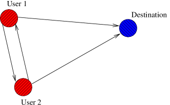
Figure 1: A Cooperative Multiple Access Channel (MAC). Arrows between two nodes illustrate that both nodes communicate between each other.

A challenging channel model is the BF[3] frequency non-selective Single-Input Single-Output (SISO) channel. When the fading gain is constant over a codeword and no cooperation is used, the resulting word error rate curve (displaying the logarithm of the error rate versus the average signal-to-noise ratio (SNR) in dB) has the same high-SNR slope as for uncoded transmission: the corresponding diversity order equals one. The potential diversity increase brought by cooperative techniques allows to save much transmit energy at a given error rate. BF channels are a realistic model for a number of channels affected by slowly varying fading and flat fading is assumed in order to isolate the effect of cooperative diversity.

The specific task of the relay is determined by the strategy or protocol. In the case Decode and Forward (DF), the relay first decodes and then re-encodes the message before sending it to the destination. A variant of DF is coded cooperation, where the relay decodes the message received from the source, and then transmits additional parity bits of the message, resulting in a more spectral efficient strategy [22], compared to a traditional DF protocol. Instead of SNR accumulation (logarithmic rise of mutual information with received power from the relay) at the destination, we get information accumulation (linear rise of mutual information with received power from the relay) [46]. It has been shown in [23] that the outage probability [3], [33] of coded cooperation for half-duplex BF channels is smaller than for repetition-based protocols. Moreover, the concept of coded cooperation can be used in more complex strategies, such as Amplify-Decode-Forward [2], where the relay can choose between DF and AF. So finally, replacing the decode-and-repeat part in any protocol by this more intelligent “information adding” strategy improves the outage probability performance. As a consequence, constructing a near-outage channel code for a coded cooperation scenario results in a competitive error-correcting code in terms of error-rate performance vs. SNR for a given rate $R$.

Up till now, coded cooperation has mainly been implemented using rate-compatible convolutional codes [22]. The main drawback of these codes is that the WER increases with the logarithm of block length to the power $d$ where $d$ is the diversity order [6], [7]. The WER of practical near-outage codes should be independent of the block length in order to approach the outage probability limit [16], [17]. The solution is to use capacity-achieving codes, for example LDPC codes [36]. LDPC codes designed for the special case of a cooperative channel have been reported for the Gaussian channel by Razaghi and Yu [34], [35] and by Chakrabarti et al. [9]. For the block-fading channel however, there is still a lack of a near-outage LDPC code. Hu et al. [20] also designed LDPC codes for the Gaussian relay channel, whereafter they applied this random LDPC code to a BF relay channel. Unfortunately, a random code does not perform very well on a BF relay channel, because it has not the structure to achieve full diversity, as shown by Boutros et al. [5] and as will be explained in the rest of the paper.

In Section III, this paper analyzes the outage probability for binary phase shift keying (BPSK) modulations and derives a coding rate limitation that is necessary for the protocol to have diversity two, valid for all discrete alphabets. Deriving a code structure for coded cooperation will be treated in the second part of the paper. The aim of coded cooperation is to send a codeword over two independent fading paths and the relay must be able to decode after receiving the first part of the codeword. An error-correcting code must therefore exhibit two properties: full-diversity and rate-compatibility. This paper derives a new code structure satisfying both properties. Often [13, 14, 15], perfect source-relay channels are assumed when designing error-correcting codes. These codes can be extended immediately to codes for cooperative systems with non-perfect source-relay channels using the proposed rate-compatible structure from this paper. We also determine density evolution equations to obtain a lower bound on the WER of the LDPC ensemble. The density evolution analysis can also be used to optimize the degree distributions, which will be discussed briefly, but this is not the topic of the paper.

Channel-State Information (CSI) is assumed at the decoder. We consider half-duplex devices, assuming that simultaneously receiving and transmitting data in the same frequency-band is too complicated due to the limited isolation of directional couplers. In addition, we also restrict the protocol to be orthogonal since we transmit at low rates (we use Binary Phase-Shift Keying (BPSK)). The proposed code construction can nevertheless be used in more complex non-orthogonal protocols, where one can achieve more coding gain in high-rate scenarios[1].

II System model and notation

As mentioned in the introduction, the devices are half-duplex and users transmit in non-overlapping time slots. The transmission of a codeword is organized in two frames which constitute one block. We denote the transmission of user $u$, $u=1,2$, in frame $m$, $m=1,2$, by $X_{u,m}$. The pair $(C_{u,1},C_{u,2})$ denotes the codeword of user $u$. In the first frame of a block, each user broadcasts the first part of its encoded data to the other user and to the destination. In the second frame, users either cooperate or send additional parity bits related to their own information message, depending on whether they are able to decode the transmissions in the first frame. The decoding failure is detected by the relaying user via a Cyclic Redundancy Check (CRC) code or any other intelligent detection scheme. There are 4 cases to be distinguished, as summarized in Fig. 2: in case 1, both users have successfully decoded the information from the other user; in case 2, none of the users has been able to decode the information from the other user; in case 3 (case 4), only user 2 (user 1) has successfully decoded the information from the other user. Methods are known allowing the destination to detect which of these 4 cases has occurred [21].

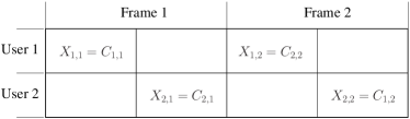
(a) Case 1. Both interuser transmissions are successfully decoded. Each user cooperates in the second frame.

(b) Case 2. Both interuser communications failed. Each user sends its own parity bits in the second frame.

(c) Case 3. User2-to-User1 communication failed. In the second frame, user 1 sends its own parity bits and user 2 cooperates with user 1.

(d) Case 4. User1-to-User2 communicatino failed. In the second frame, user 2 sends its own parity bits and user 1 cooperates with user 2.

Figure 2: The 4 cases encountered in coded cooperation are listed above.

A codeword will consequently be split over 2 frames. We consider codewords to have a total length equal to $N$ binary digits, where $N=N_{1}+N_{2}$, and $N_{1}$ and $N_{2}$ denote the length of the first and second part of the codeword. We define the level of cooperation, $\beta$, as the ratio $N_{2}/N$.
We denote the transmitter of a frame, which can be user 1 or user 2, by $s$ and the receiver of a frame, which can be user 1, user 2 or the destination, by $r$. Transmitted symbols of user 1 will be denoted $x_{1}[i]$ where $i$ is the symbol time index, $i\in\{1,\ldots,N\}$. Similarly, transmitted symbols of user 2 are denoted $x_{2}[i]$. The transmitted symbols are chosen from a BPSK alphabet, $x_{s}[i]\in\{1,-1\}$. Received symbols will be denoted $y_{sr}[i]$ for received symbols from transmitter $s$ to receiver $r$. The received symbol is given by

$$y_{sr}[i]=\alpha_{sr}x_{s}[i]+z_{r}[i],$$ (1)

where $z_{r}[i]\sim\mathcal{N}(0,\sigma^{2})$ are independent noise samples and $\alpha_{sr}\in\mathbb{R}^{+}$ is the Rayleigh distributed fading gain between sender $s$ and receiver $r$, with normalized second order moment, $\mathbb{E}[\alpha_{sr}^{2}]=1$. The fading coefficient $\alpha_{sr}$ is assumed to be constant during 2 frames. Note that this channel model is memoryless [10] and satisfies the channel symmetry condition, $p(y_{sr}[i]|\alpha_{sr},x_{s}[i]=1)=p(-y_{sr}[i]|\alpha_{sr},x_{s}[i]=-1)$. Each terminal is transmitting at a constant enery per symbol $E_{s}$, which is related to the energy per information bit $E_{b}$ by $E_{s}=R_{c}E_{b}$ (BPSK). The total energy per information bit-to-noise ratio is specified by $E_{b}/N_{0}$.

We focus on binary LDPC codes $\mathcal{C}[N,K]_{2}$ with block length $N$, dimension $K$, and coding rate $R_{c}=K/N$. Regular LDPC ensembles are characterized by the pair $(d_{b},d_{c})$, where $d_{b}$ is the maximum bitnode degree and $d_{c}$ is the maximum checknode degree. Irregularity is introduced through the standard polynomials $\lambda(x)$ and $\rho(x)$ [38]:

$$\lambda(x)=\sum_{i=2}^{d_{b}}{\lambda_{i}x^{i-1}},~{}~{}~{}~{}\rho(x)=\sum_{i=2}^{d_{c}}{\rho_{i}x^{i-1}}.$$

where $\lambda(x)$ and $\rho(x)$ are the left and right degree distributions from an edge perspective. In Section V the polynomials $\mathring{\lambda}(x)$ and $\mathring{\rho}(x)$, which are the left and right distributions from a node perspective, will also be adopted:

$$\mathring{\lambda}(x)=\sum_{i=2}^{d_{b}}{\mathring{\lambda}_{i}x^{i-1}},~{}~{}~{}~{}\mathring{\rho}(x)=\sum_{i=2}^{d_{c}}{\mathring{\rho}_{i}x^{i-1}}.$$

In this paper, not all bit nodes and check nodes in the Tanner graph will be treated equally. To elucidate the different classes of bit nodes and check nodes, a compact representation of the Tanner graph, adopted from [8] and also known as protograph representation [42], will be used. In this compact Tanner graph, bit nodes and check nodes of the same class are merged into one node.

Definition 1

The diversity order attained by a code $\mathcal{C}$ is defined as

$$d=-\lim_{\gamma\rightarrow\infty}\frac{\log P_{e}}{\log\gamma},$$

where $P_{e}$ is the word error rate after decoding.

Definition 2

An error-correcting code is said to have full diversity if $d=N_{u}$, where $N_{u}$ is the number of cooperating users.

Notice that the above definition assumes Rayleigh distributed single antenna channels. According to the blockwise Singleton bound [25], [30], the coding rate for an $n$-order full-diversity code is upper bounded by $R_{cmax}=1/n$. Hence, in a 2-user scenario we get $R_{c}\leq 0.5$.

III Outage Probability Analysis

The word error rate of practical systems is, in the limit of large block length, lower bounded by the information outage probability

$$P_{out}=P\big{(}I(\alpha,\gamma)<R\big{)},$$

where $I(\alpha,\gamma)$ is the instantaneous mutual information as a function of a certain fading gain $\alpha$ and average SNR $\gamma$, $\gamma=\frac{E_{s}}{N_{0}}=\frac{1}{2\sigma^{2}}$, where $E_{s}$ is the symbol energy. This definition remains valid for a channel model as described in (1), but then $\alpha$ is the set of fading gains over a codeword and $\gamma$ is the set of average received SNRs. The rate $R$ is the spectral efficiency of a user, only taking into account its timeslots, hence not the average spectral efficiency. The diversity order of the outage probability limit is the same as the order attained by a full-diversity channel code[16]. It is our aim in this paper to approach the outage probability limit for a range of values of the spectral efficiency $R$. Since we use BPSK signaling, the spectral efficiency $R$ is identical to $R_{c}$.

The outage probability analysis of coded cooperation with a Gaussian alphabet has been made in [23]. Here, the analysis considers BPSK signaling, leading to an important conclusion in Corollary 1 at the end of this section. The stated corollary is also valid for larger discrete alphabets.
The average mutual information of a SISO channel with received signal $y$, conditioned on the channel realization $\alpha$, is determined by the following well-known formula[44]:

$$I(X;Y|\alpha)=1-\mathbb{E}_{Y|\alpha}\left\{\log_{2}\left(1+\exp\left[\frac{-2y\alpha}{\sigma^{2}}\right]\right)\right\},$$ (2)

where $\mathbb{E}_{Y|\alpha}$ is the mathematical expectation over $Y$ given $\alpha$. The outage event of a point-to-point link is defined by the mutual information of that link being less than its transmission rate. The outage event $E_{o}$ of the relay channel is determined by a specific region in the multidimensional space of instantaneous signal-to-noise ratios. Next, we give the exact definition of $E_{o}$ for coded cooperation with BPSK modulation. We shorten the notation $I(X_{i};Y_{j}|\alpha_{ij})$ to $I_{ij}$.

Proposition 1

In coded cooperation for a two-user MAC with BPSK signaling, the outage event $E_{o}$ related to user 1 is expressed as follows:

$$E_{o} \stackrel{{\scriptstyle a)}}{{=}} \left[\left(I_{12}>\frac{R}{1-\beta}\right)\cap\left(I_{21}>\frac{R}{1-\beta}\right)\cap\left(I_{1d}\left(1\right)<R\right)\right]$$

$$\cup \left[\left(I_{12}<\frac{R}{1-\beta}\right)\cap\left(I_{21}<\frac{R}{1-\beta}\right)\cap\left(I_{1d}\left(2\right)<R\right)\right]$$

$$\cup \left[\left(I_{12}>\frac{R}{1-\beta}\right)\cap\left(I_{21}<\frac{R}{1-\beta}\right)\cap\left(I_{1d}\left(3\right)<R\right)\right]$$

$$\cup \left[\left(I_{12}<\frac{R}{1-\beta}\right)\cap\left(I_{21}>\frac{R}{1-\beta}\right)\cap\left(I_{1d}\left(4\right)<\frac{R}{1-\beta}\right)\right],$$

where

$$I_{12} \stackrel{{\scriptstyle b)}}{{=}} 1-\mathbb{E}_{Y|\alpha_{12}}\left\{\log_{2}\left(1+\exp\left[\frac{-2y_{12}\alpha_{12}}{\sigma_{12}^{2}}\right]\right)\right\},$$ (3)

$$I_{21} \stackrel{{\scriptstyle b)}}{{=}} 1-\mathbb{E}_{Y|\alpha_{21}}\left\{\log_{2}\left(1+\exp\left[\frac{-2y_{21}\alpha_{21}}{\sigma_{21}^{2}}\right]\right)\right\},$$ (4)

and where $I_{1d}(1)$ is $I_{1d}$ in case $i$. For each of the cases considered in Fig. 2, the mutual information $I_{1d}$ can be calculated as follows:

Case 1:

$$I_{1d}(1) \stackrel{{\scriptstyle c)}}{{=}}1-(1-\beta)\ \mathbb{E7}_{Y|\alpha_{1d}}\left\{\log_{2}\left(1+\exp\left[\frac{-2y_{1d}\alpha_{1d}}{\sigma_{1d}^{2}}\right]\right)\right\}$$

$$-\beta\ \mathbb{E}_{Y|\alpha_{2d}}\left\{\log_{2}\left(1+\exp\left[\frac{-2y_{2d}\alpha_{2d}}{\sigma_{2d}^{2}}\right]\right)\right\}.$$ (6)

Case 2:

$$I_{1d}(2) \stackrel{{\scriptstyle c)}}{{=}}1-\mathbb{E}_{Y|\alpha_{1d}}\left\{\log_{2}\left(1+\exp\left[\frac{-2y_{1d}\alpha_{1d}}{\sigma_{1d}^{2}}\right]\right)\right\}.$$ (7)

Case 3:

$$I_{1d}(3) \stackrel{{\scriptstyle c)}}{{=}}1-(1-\beta)\ \mathbb{E}_{Y|\alpha_{1d}}\left\{\log_{2}\left(1+\exp\left[\frac{-2y_{1d}\alpha_{1d}}{\sigma_{1d}^{2}}\right]\right)\right\}$$

$$-\beta\ \mathbb{E}_{Y^{\prime}|{\alpha_{1d}\alpha_{2d}}}\left\{\log_{2}\left(1+\exp\left[\frac{-2(y^{\prime})(\alpha_{1d}^{2}+\alpha_{2d}^{2})^{3/2}}{\sigma_{1d}^{2}\alpha_{1d}^{2}+\sigma_{2d}^{2}\alpha_{2d}^{2}}\right]\right)\right\},$$ (8)

$$y^{\prime} =\frac{(\alpha_{1d}y_{1d}+\alpha_{2d}y_{2d})}{\sqrt{\alpha_{1d}^{2}+\alpha_{2d}^{2}}}.$$

Case 4:

$$I_{1d}(4) \stackrel{{\scriptstyle c)}}{{=}}1-\mathbb{E}_{Y|\alpha_{1d}}\left\{\log_{2}\left(1+\exp\left[\frac{-2y_{1d}\alpha_{1d}}{\sigma_{1d}^{2}}\right]\right)\right\}.$$ (9)

Proof.

a)

is the union of four events associated to the four cases considered in Fig. 2. Each case in $E_{o}$ involves the intersection with an outage event where the mutual information between a user and the destination is below the rate $R$, except for case 4, where only the first frame is dedicated to user 1.

b)

follows directly from (2).

c)

uses the fact that the two frames in a block behave as parallel Gaussian channels whose capacities add together. Of course, both frames timeshare a time-interval, which gives a weight to each capacity term [10, Section 9.4], [43, Section 5.4.4].

(1)

follows from maximum ratio combining [43] at the destination during the second frame.

∎

The outage probability is obtained by integrating the joint probability distribution $p(\alpha_{12},\alpha_{21},\alpha_{1d},\alpha_{2d})$ over the volume defined by $E_{o}$:

$$P_{out}=\iiint_{E_{o}}p(\alpha_{12},\alpha_{21},\alpha_{1d},\alpha_{2d})~{}\mathrm{d}\alpha_{12}\mathrm{d}\alpha_{21}\mathrm{d}\alpha_{1d}\mathrm{d}\alpha_{2d}.$$

Just as for the Gaussian modulation, there is only one free parameter $\beta$ because $R$ and $\gamma$ are fixed by the protocol and the physical environment. Hence, given R and $\gamma$, one can optimize the value of $\beta$. For example, notice that for a low-SNR interuser channel, the outage probability improves while taking $\beta$ smaller than $0.5$ due to the enhanced protection of the source-relay channel. On the other hand, a $\beta$ smaller than $0.5$ results in lower achievable coding rates, as proved in Corollary 1. The optimization of $\beta$, as already undertaken in [23] for Gaussian modulations, is not within the subject of this paper.

There is an important conclusion to draw from the analysis of Prop. 1:

Corollary 1

In coded cooperation over a block-fading channel for the 2-user MAC with a cooperation level $\beta$, transmitting at a coding rate greater than $\textrm{min}(\beta,(1-\beta))$ renders a single order diversity.

Proof.

A necessary condition for coded cooperation to achieve full diversity over a block-fading channel, is that it achieves full diversity over a Block Erasure Channel (BEC)[27], because a BEC is an extremal case of a block-fading channel. We will show that this condition is not satisfied for coding rates greater than $\textrm{min}(\beta,(1-\beta))$. In a BEC, the fading gain $\alpha$ takes two possible values $\{0,+\infty\}$. An outage event on a point-to-point channel is defined by the fading gain $\alpha$ being zero. As a consequence, the possible values of the BPSK capacity on a BEC are confined to zero or one. Hence, for the two-user MAC, the mutual information $I_{1d}$ related to case 1 belongs to $\{1,\beta,(1-\beta),0\}$. A double diversity order is equivalent to stating that two outage events are necessary to lose the transmitted codeword. Take the scenario where the user1-to-destination channel has fading gain zero and the user2-to-destination channel has fading gain $\infty$. In this scenario, the mutual information $I_{1d}$ is equal to $\beta$. All coding rates higher than $\beta$ will limit the diversity order of the outage probability to one, since only one channel in outage is enough to lose the codeword. From a similar reasoning, it is shown that $R_{c}$ must be smaller than $(1-\beta)$. This corollary is also valid for signaling strategies with $M$ constellation points. ∎

In the sequel, if not otherwise stated, we assume a rate equal to $R_{c}=\frac{1}{3}$. From Corollary 1, we know that the level of cooperation must at least belong to $\beta\in[\frac{1}{3},~{}\frac{2}{3}]$. We stress on the fact that the proposed code construction is very flexible in parameters such as the block length and the coding rate. We will use $\beta=0.5$ throughout this paper, which allows the broadest range of coding rates according to Corollary 1. We illustrate this in the numerical results by showing the WER performance of an LDPC code whose coding rate $R_{c}$ approaches $1/2$.

IV Full-diversity Low-Density coding for coded cooperation

Codewords in coded cooperation are split over 2 frames. The first part of a codeword, transmitted during the first frame should protect information on the noisy source-relay channel. Consequently, a channel code, compatible with two distinct rates is to be devised. In non-cooperative communications, this property is known as rate-compatibility where parity bits of higher rate codes are embedded in those of lower rate codes [19]. The advantage is that all codes can be encoded/decoded using a single encoder/decoder.
Rate-compatibility in the context of LDPC codes was first introduced by Li et al. [29] and Ha et al. [18] and further elaborated for example in [45]. Two techniques have been used: puncturing and extending. A fraction of parity bits of a mother code could be punctured to obtain higher rate codes. However, the resulting rate range is limited because the deletion of too many bits has a negative effect on decoding via belief propagation. To obtain a more dynamic range in rates, the technique of extending has been used. The extension is made by adding extra parity bits as illustrated in Fig. 3, where the overall code is the intersection of two constituent codes defined by $H_{2}$ and $H_{1}$ padded with zeros on the right.

Figure 3: Parity-check matrix of a rate-compatible LDPC code obtained by the extension of higher rate codes. Symbols are split into three classes: $i$ for the information bits, $1p$ and $2p$ for two classes of parity bits. The classes $i$ and $1p$ are transmitted by the source in frame 1. Parity bits $2p$ are transmitted in the second frame, for example by the relay after successful decoding of the first frame.

For simplicity, we only used the technique of extending to acquire rate-compatibility, but this may be further optimized by combining puncturing and extending via known techniques [29, 18, 45].

IV-A Full-diversity LDPC codes

In coded cooperation, 4 cases occur depending on the success of the transmission in the first frame. In each of the cases, the destination has other log-likelihood ratios at the input of the decoder. In the following proposition, we will show that it is sufficient to guarantee that the decoder at the destination achieves full diversity in case 1.

Proposition 2

In coded cooperation on a cooperative MAC, a code $\mathcal{C}$ attains full diversity, if and only if full diversity is attained in case 1.

Proof.

The WER after decoding $P_{e}$ can be split as follows

$$P_{e}=\sum_{i=1}^{4}P(\textrm{case i})P(e|\textrm{case i}).$$ (10)

The probability that a certain case occurs, depends on the success of decoding two point-to-point channels, so that it is easy to derive that:

$$P(\textrm{case 1}) = (1-\frac{c}{\gamma})(1-\frac{c}{\gamma})$$ (11)

$$P(\textrm{case 2}) = (\frac{c}{\gamma})(\frac{c}{\gamma})$$ (12)

$$P(\textrm{case 3}) = (1-\frac{c}{\gamma})(\frac{c}{\gamma})$$ (13)

$$P(\textrm{case 4}) = (\frac{c}{\gamma})(1-\frac{c}{\gamma}),$$ (14)

where $c$ is a positive constant. To have $P_{e}\propto\frac{1}{\gamma^{2}}$, the following conditions apply:

$$P(e|\textrm{case 1}) \propto \frac{1}{\gamma^{2}},$$ (15)

$$P(e|\textrm{case 2}) \propto 1,$$ (16)

$$P(e|\textrm{case 3}) \propto \frac{1}{\gamma},$$ (17)

$$P(e|\textrm{case 4}) \propto \frac{1}{\gamma}.$$ (18)

Eqs. (16), (17) and (18) are automatically satisfied, so that the only nessecary and sufficient condition is (15). ∎

Due to Proposition 2, we will assume in the following analysis the occurrence of case 1 where the transmission on the interuser channel in the first frame has been successful and both users are cooperating in the second frame. Full-diversity coding on a relay channel must cope with block erasures. Consider the coding structure plotted in Fig. 3. If all parity bits $2p$ are erased due to deep fading in frame 2, then the decoder should be capable to retrieve information bits $i$ thanks to $H_{1}$ and possibly recompute $2p$ thanks to $H_{2}$. Unfortunately, under deep fading in frame 1, a structure with a randomly generated $H_{2}$, as in Fig. 3, cannot guarantee the retrieval of the information bits through $H_{2}$. The aim of this section is to explain how $H_{2}$ can be tuned in order to have full diversity for any left and right degree distribution and for any block length.

To the destination, it appears as if one source has sent its codeword over a point-to-point BF channel in case 1. Therefore, we take the constituent code defined by $H_{2}$ to be a full-diversity LDPC code (referred to as root-LDPC code) as constructed by Boutros et al. in [8], [5] for non-cooperative single-antenna channels with two or more fading states per codeword. The Tanner graph notation for the root-LDPC code is given in Fig. 4. This notation is essential for the analysis because we seek full diversity under iterative decoding.

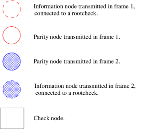
Figure 4: Notation for the Tanner graph of a full-diversity LDPC code.

Full diversity of a root-LDPC structure is created by rootchecks, a special type of checknodes in the Tanner graph. As shown in Fig. 5, the root and the leaves of this special checknode do not belong to the same frame. When the rootbit is in frame 1, the leavebits are in frame 2, and vice versa. Using the limiting case of a Block-Erasure Channel, it is easy to verify that a rootbit is determined via its rootcheck when its own frame is erased.

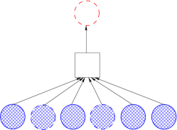
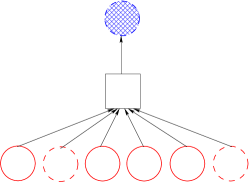
Figure 5: Two types of rootchecks. On the left-hand side, the rootbit belongs to frame 1 and the leavebits belong to frame 2. The symmetric case where channel states are switched is shown at the right-hand side.

The complete root-LDPC structure is built after splitting information bits into two classes, denoted $1i$ and $2i$, and parity bits into two classes, denoted $1p$ and $2p$. The checknodes are cut into two classes denoted $3c$ and $4c$. The classes $3c$ and $4c$ consist of rootchecks for information bits $1i$ and $2i$ respectively. The complete root-LDPC structure including all types of nodes is illustrated in Figs. 6 and 7. Rootchecks are translated into two identity matrices (or permutation matrices in general) inside the parity-check matrix in Fig. 7.

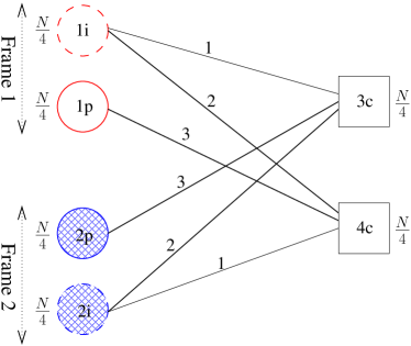
Figure 6: Tanner graph of a full-diversity LDPC code of length $N$ and rate $\frac{1}{2}$. This compact graph representation has been adopted from [8], [5], it is also known as protograph representation [42]. The integers labeling the edges of the Tanner graph indicate the degree of a node along those edges for a regular (3,6) root-LDPC code. The binary elements are split into four classes of each $\frac{N}{4}$ bits. The checknodes are cut into two classes of $\frac{N}{4}$ checks.

The proof of full-diversity for block-Rayleigh fading can be found in [8]. Note that the diversity order of the root-LDPC code does not depend on the right or left degree distributions. For simplicity, we only showed a regular (3,6) structure in Fig. 6.

Figure 7: Parity-check matrix of a rate $\frac{1}{2}$ root-LDPC code.

Note that although this code is natural for the point-to-point BF channel, it isn’t for the cooperative MAC. The source is sending only half of its information bits to the relay, who is supposed to decode all the information bits. This sounds counter-intuitive and we are the first to apply this concept in cooperative communications. Although it is counter-intuitive, it is necessary to achieve full diversity with iterative decoding, as explained above.

For asymptotic code lengths, multi-edge type messages propagate in the root-LDPC graph [39]. One has to choose between two different root-LDPC ensembles. If we refer to the Tanner graph in Fig. 6, the two ensembles are distinguished as follows: (i) The first ensemble is built by two random edge permutations (edge interleavers) connecting $3c$ to ($2i$, $2p$) and $4c$ to ($1i$, $1p$) respectively. This is equivalent to the random generation of two low-density matrices ($H_{2i}$, $H_{2p}$) and ($H_{1i}$, $H_{1p}$) in the parity-check matrix shown in Fig. 7. (ii) The second ensemble is built by four random edge permutations $3c-2i$, $3c-2p$, $4c-1i$, and $4c-1p$. In the root-LDPC parity-check matrix, this is equivalent to building seperately the four submatrices $H_{2i}$, $H_{2p}$, $H_{1i}$, and $H_{1p}$. For simplicity reasons, mainly in the density evolution (DE) analysis, we adopt the first root-LDPC ensemble as part of the full-diversity cooperative code proposed in the next subsection.

IV-B Rate-compatible full-diversity LDPC codes

The difference with [8] is that our code construction must take into account the protocol of coded cooperation, i.e., the 4 different cases, to perform well on this channel. Furthermore, the optimized degree distributions of our code construction will be different from [8], because of the multi-edge type structure [39] of this code construction. The structure of an LDPC ensemble for coded cooperation is derived by joining the rate-compatibility property and the full-diversity property. The global parity-check matrix is obtained by embedding the root-LDPC matrix (Fig. 7) into the rate-compatible matrix (Fig. 3). This leads to an asymmetric code where class $1i$ may have a higher coding gain than class $2i$. Therefore, we propose an extension to the “extending” technique, due to the fact that we split the information bits over two frames, which is a new phenomenon. To get a balanced structure, we replace the zero-padded $H_{1}$ by the direct sum of two rate $R_{1}$ codes defined by $H_{1s}$ and $H_{1r}$ as illustrated in Fig. 8. Thus, the constituent code $H_{1s}$ protects bits $1i$ and $1p$ via extra parity bits $p_{1}^{\prime}$. Similarly, in the second frame, extra parity bits $p_{2}^{\prime}$ are generated from $2i$ and $2p$. The bottom of the global parity-check matrix simply includes the root-LDPC structure, connecting ($1i$, $1p$) to ($2i$, $2p$). For simplicity we can assume that $H_{1s}$ and $H_{1r}$ belong to the same rate $R_{1}$ random LDPC ensemble, defined by the degree distributions $(\lambda_{1}(x),\rho_{1}(x))$. Hence, if the degree distribution of the root-LDPC is $(\lambda_{2}(x),\rho_{2}(x))$, we refer to the rate-compatible root-LDPC (RCR-LDPC) as a $(\lambda_{1}(x),\rho_{1}(x),\lambda_{2}(x),\rho_{2}(x))$ code. The Tanner graphs of a regular $(3,9,3,6)$ LDPC code and an irregular $(\lambda_{1}(x),\rho_{1}(x),\lambda_{2}(x),\rho_{2}(x))$ code are shown in Figs. 9 and 10. Since we guarantee full diversity via a root-LDPC with a fixed rate $\frac{1}{2}$, the global coding rate of the RCR-LDPC code observed at the destination is $R_{c}=\frac{R_{1}}{2}$. As a consequence, the global coding rate $R_{c}$ can be easily varied through $R_{1}$ and is upper limited by $0.5$.

Figure 8: Parity-check matrix of a RCR-LDPC code for coded cooperation. The upper coding rate associated to $H_{1s}$ and $H_{1r}$ is $R_{1}=\frac{2}{3}$, the bottom root-LDPC coding rate is $\frac{1}{2}$, and the overall coding rate is $R_{c}=\frac{R_{1}}{2}=\frac{1}{3}$.

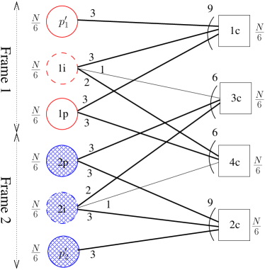
Figure 9: Tanner graph of a regular $(3,9,3,6)$ RCR-LDPC code for coded cooperation. We see that the average bit degree is $\bar{d_{b}}=5$ and the average check degree is $\bar{d_{c}}=\frac{15}{2}$ which results in $R_{c}=1-\frac{\bar{d_{b}}}{\bar{d_{c}}}=\frac{1}{3}$.

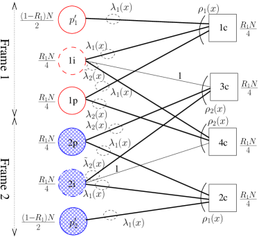
Figure 10: Tanner graph of an irregular RCR-LDPC code for coded cooperation. The binary elements are split into six classes, $p_{1}^{\prime}$ and $p_{2}^{\prime}$ of each $\frac{(1-R_{1})N}{2}$ bits and $1i$, $1p$, $2i$, and $2p$ of each $\frac{R_{1}N}{4}$ bits. The checknodes are cut into four classes of $\frac{R_{1}N}{4}$ checks.

Due to the identity matrices inside the parity-check matrix, new polynomials $\tilde{\lambda}_{2}(x)$ appear in Fig. 10 in the connections $1i-4c$ and $2i-3c$, as illustrated in Fig. 11.

Figure 11: Transition from a traditional representation, characterized by an edge distribution polynomial $\lambda(x)$, towards a representation where one edge per bitnode is isolated resulting in a new degree distribution $\tilde{\lambda}(x)$.

Proposition 3

In a Tanner graph with a left degree distribution $\lambda(x)$, isolating one edge per bitnode yields a new left degree distribution described by the polynomial $\tilde{\lambda}(x)$:

$$\tilde{\lambda}\left(x\right)=\sum_{i}{\tilde{\lambda}_{i}\ x^{i-1}},~{}~{}~{}~{}~{}~{}\tilde{\lambda}_{i-1}=\frac{\lambda_{i}(i-1)/i}{\sum_{j}{\lambda_{j}(j-1)/j}}.$$ (19)

Proof.

Let us define $T_{\textrm{bit,}i}$ as the number of edges connected to a bitnode of degree $i$. Similarly, the number of all edges is denoted $T_{\textrm{bit}}$. From Section II, we know that $\lambda(x)=\sum_{i=2}^{d_{bmax}}\lambda_{i}x^{i-1}$ expresses the left degree distribution, where $\lambda_{i}$ is the fraction of all edges in the Tanner graph, connected to a bitnode of degree $i$. So finally $\lambda_{i}=\frac{T_{\textrm{bit,}i}}{T_{\textrm{bit}}}$. A similar reasoning can be followed to determine $\tilde{\lambda}_{i}$:

$$\tilde{\lambda}_{i-1} \stackrel{{\scriptstyle a)}}{{=}} \frac{T_{\textrm{bit,}i}-\frac{\lambda_{i}}{i}T_{\textrm{bit}}}{T_{\textrm{bit}}-\sum_{j}{\frac{\lambda_{j}}{j}T_{\textrm{bit}}}}$$

$$\stackrel{{\scriptstyle b)}}{{=}} \frac{\lambda_{i}T_{\textrm{bit}}-\frac{\lambda_{i}}{i}T_{\textrm{bit}}}{T_{\textrm{bit}}-\sum_{j}{\frac{\lambda_{j}}{j}T_{\textrm{bit}}}}$$

$$= \frac{\lambda_{i}-\frac{\lambda_{i}}{i}}{\sum_{j}{\frac{\lambda_{j}}{j}j}-\sum_{j}{\frac{\lambda_{j}}{j}}}$$

$$= \frac{\frac{\lambda_{i}}{i}(i-1)}{\sum_{j}{\frac{\lambda_{j}}{j}(j-1)}}.$$

a)

$\sum_{j}{\frac{\lambda_{j}}{j}T_{\textrm{bit}}}$ is equal to the number of edges that are removed which is equal to the number of bits.

b)

$\lambda_{i}T_{\textrm{bit}}$ is equal to the number of edges connected to a bit of degree $i$.

∎

In Section V, we will also use $\tilde{\rho}\left(x\right)$, which is defined similarly as $\tilde{\lambda}\left(x\right)$.

Proposition 4

Consider a $(\lambda_{1}(x),\rho_{1}(x),\lambda_{2}(x),\rho_{2}(x))$ RCR-LDPC code for coded cooperation transmitted on a 2-user block-fading cooperative MAC. Then, under iterative belief propagation decoding, the RCR-LDPC code has full diversity.

Proof.

Let $\Lambda_{i}^{a}$, $i=1\ldots d_{c}-1$ denote the input log-ratio probabilistic messages to a checknode $\Phi$ of degree $d_{c}$. The output message $\Lambda^{e}$ for belief propagation is [37]

$$\Lambda^{e}=2\textrm{th}^{-1}\left(\prod_{i=1}^{d_{c}-1}\textrm{th}\left(\frac{\Lambda_{i}^{a}}{2}\right)\right),$$

where $\textrm{th}(x)$ denotes the hyperbolic-tangent function. Superscripts $a$ and $e$ stand for a priori and extrinsic, respectively. To simplify the proof, we show that the suboptimal min-sum decoder yields a diversity order $2$. For a min-sum decoder, the output message produced by a checknode $\Phi$ is now

$$\Lambda^{e}=\min{(|\Lambda_{i}^{a}|)}\prod_{i=1}^{d_{c}-1}\textrm{sign}(\Lambda_{i}^{a}).$$

An information bit $\vartheta$ of class $1i$ of degree $d_{b}$ has $\Lambda_{0}=\frac{2\alpha_{sr}y_{sr}}{\sigma^{2}}$ where $\Lambda_{0}$ is the log-likelihood ratio coming from the likelihood $p(y_{sd}|\vartheta)$. It also receives $d_{b}$ messages: $\Lambda_{1,i}^{e}$, $i=1\ldots d_{b1}$ and $\Lambda_{2,i}^{e}$, $i=1\ldots d_{b2}$, $d_{b}=d_{b1}+d_{b2}$, from its neighbouring checknodes in the constituent codes $H_{1s}$ and $H_{2}$ respectively. The total a posteriori message corresponding to $\vartheta$ is $\Lambda=\Lambda_{0}+\sum_{i=1}^{d_{b1}}{\Lambda_{1,i}^{e}}+\sum_{i=1}^{d_{b2}}{\Lambda_{2,i}^{e}}$. In [8] it is proven that full-diversity is achieved if and only if $\Lambda$ behaves as $a\alpha_{1d}^{2}+b\alpha_{2d}^{2}$, where $a,b>0$.

The addition of $\sum_{i=1}^{d_{b1}}\Lambda_{1,i}^{e}$ cannot degrade the error probability $P_{e}(1i)$ because the convolution with the density of messages from $H_{1s}$ can only physically upgrade the resulting density. Thus, it is sufficient to prove that message $\Lambda_{0}+\sum_{i=1}^{d_{b2}}\Lambda_{2,i}^{e}$ exhibits full diversity, i.e., behaves as $a\alpha_{1d}^{2}+b\alpha_{2d}^{2}$, which is proven in [8]. ∎

V Density Evolution on the Block-Fading Relay Channel

Richardson and Urbanke [36, 37] established that, if the block length is large enough, (almost) all codes in an ensemble of codes behave alike, so the determination of the average behavior is sufficient to characterize a particular code behavior. This average behavior converges to the cycle-free case if the block length augments and it can be found in a deterministic way through density evolution (DE). The evolution trees represent the local neighborhood of a bitnode in an infinite length code whose graph has no cycles, hence incoming messages to every node are independent.

V-A Interuser channel

To determine the density of messages propagating in the graph of the constituent code $H_{1s}$, the following notation is used:

$$d_{sr}^{m}(x) =$$ density of message from a bitnode to

$$\textrm{ a checknode in the $\textrm{m}^{\textrm{th}}$ iteration}.$$

$$\mu_{sr}(x) =$$ density of the likelihood of

the source-relay channel.

Let $X_{1}\sim p_{1}(x)$ and $X_{2}\sim p_{2}(x)$ be two independent real random variables. The density function of $X_{1}+X_{2}$ is obtained by convolving the two original densities, written as $p_{1}(x)\otimes p_{2}(x)$. The notation $p(x)^{\otimes n}$ denotes the convolution of $p(x)$ with itself $n$ times.

Let $X_{1}\sim p_{1}(x)$ and $X_{2}\sim p_{2}(x)$ be two independent real random variables. The density function $p(y)$ of the variable $Y=2\ \textrm{th}^{-1}\left(\textrm{th}\left(\frac{X_{1}}{2}\right)\textrm{th}\left(\frac{X_{2}}{2}\right)\right)$, obtained through a checknode with $X_{1}$ and $X_{2}$ at the input, is obtained through the R-convolution [37], written as $p_{1}(x)\odot p_{2}(x)$. The notation $p(x)^{\odot n}$ denotes the R-convolution of $p(x)$ with itself $n$ times.

To simplify the notations, we use the following definitions:

$$\lambda\left(p\left(x\right)\right)=\sum_{i}{\lambda_{i}\ p(x)^{\otimes i-1}},~{}~{}\rho\left(p\left(x\right)\right)=\sum_{i}{\rho_{i}\ p(x)^{\odot i-1}}.$$

In the next subsection we will also use the following definitions:

$$\rho\left(p\left(x\right),t\left(x\right)\right) = \sum_{i}{\left(\rho_{i}\ p(x)^{\odot i-1}\odot t(x)\right)},$$

$$\lambda^{*}\left(p\left(x\right)\right) = \lambda\left(p\left(x\right)\right)\otimes\left(p\left(x\right)\right),$$

$$\rho^{*}\left(p\left(x\right)\right) = \rho\left(p\left(x\right)\right)\odot\left(p\left(x\right)\right).$$

The first definition is necessary because of the non-linearity of the R-convolution. Therefore, the first equation is not equal to $t(x)\odot\rho\left(p\left(x\right)\right)$. The next subsection will also use the polynomials $\mathring{\rho}^{*}\left(x\right)$ and $\mathring{\lambda}^{*}\left(x\right)$ which are defined by combining the two transformations, denoted by $\mathring{(.)}$ (see introduction) and $(.)^{*}$.

Fig. 12 illustrates the local neighborhood of a bitnode in the constituent code $H_{1s}$.

Figure 12: Local neighborhood of a bitnode in the constituent code $H_{1s}$. This tree is used to determine the evolution of density $d_{sr}(x)$ of messages from a bitnode to a checknode.

The DE equation in the neighborhood of the bitnode for a $(\lambda_{1}(x),\rho_{1}(x))$ LDPC code [36] is, for all $m$,

$$d_{sr}^{m+1}(x)=\mu_{sr}(x)\otimes\lambda_{1}\bigg{(}\rho_{1}\big{(}d_{sr}^{m}(x)\big{)}\bigg{)}.$$ (20)

The threshold of a code is the minimum SNR at which a codeword can be decoded perfectly [36]. Comparing the received signal-to-noise ratio with this threshold, the relay and the source can determine whether the interuser transmissions can be decoded successfully and consequently decide what to transmit in the second frame.

V-B Overall cooperative MAC

The proposed $(\lambda_{1}(x),\rho_{1}(x),\lambda_{2}(x),\rho_{2}(x))$ root-LDPC code has 6 variable node types and 4 checknode types. Consequently, the evolution of message densities under iterative decoding has to be described through multiple evolution trees. Figs. 13, 15 and 16 show the local neighborhood of a bit node of the class $1i$. The local neighborhoods of bit nodes of the classes $1p$, and $p_{1}^{\prime}$ can be derived similarly. The local neighborhood of classes $2i$, $2p$, and $p_{2}^{\prime}$ are equivalent because of code symmetry.

To determine the density of messages, the following notation is used:

$$a_{1}^{m}(x)\textrm{, }a_{2}^{m}(x) = 1i 1c$$ density of message from to and

$$\textrm{ $2i$ to $2c$ respectively, at the $\textrm{m}^{\textrm{th}}$ iteration},$$

$$f_{1}^{m}(x)\textrm{, }f_{2}^{m}(x) = 1i 3c$$ density of message from to and

$$\textrm{ $2i$ to $4c$ respectively, at the $\textrm{m}^{\textrm{th}}$ iteration},$$

$$g_{1}^{m}(x)\textrm{, }g_{2}^{m}(x) = 1i 4c$$ density of message from to and

$$\textrm{ $2i$ to $3c$ respectively, at the $\textrm{m}^{\textrm{th}}$ iteration},$$

$$k_{1}^{m}(x)\textrm{, }k_{2}^{m}(x) = 1p 1c$$ density of message from to and

$$\textrm{ $2p$ to $2c$ respectively, at the $\textrm{m}^{\textrm{th}}$ iteration},$$

$$l_{1}^{m}(x)\textrm{, }l_{2}^{m}(x) = 1p 4c$$ density of message from to and

$$\textrm{ $2p$ to $3c$ respectively, at the $\textrm{m}^{\textrm{th}}$ iteration},$$

$$q_{1}^{m}(x)\textrm{, }q_{2}^{m}(x) = p^{\prime}_{1} 1c$$ density of message from to and

$$\textrm{ $p^{\prime}_{2}$ to $2c$ respectively in the $\textrm{m}^{\textrm{th}}$ iteration},$$

$$\mu_{i}(x) =$$ density of the likelihood of the channel

$$\textrm{ in the $i$'th frame}.$$

Note that $\mu_{2}(x)$ depends on the success or the failure of the transmissions in the first frame.

Figure 13: Local neighborhood of bitnode $1i$. This tree is used to determine the evolution of the density of messages $1i\rightarrow 1c$.

Proposition 5

The DE equations in the neighborhood of $1i$ for a $(\lambda_{1}(x),\rho_{1}(x),\lambda_{2}(x),\rho_{2}(x))$ RCR-LDPC ensemble for coded cooperation, for all $m$, are given in Eqs. (21), (22) and (23)

$$a_{1}^{m+1}(x) = \mu_{1}(x)\otimes\mathring{\lambda}_{2}\bigg{(}\tilde{\rho_{2}}\big{(}f_{1i4c}\ g_{1}^{m}(x)+f_{1p4c}\ l_{1}^{m}(x),\ f_{2}^{m}(x)\big{)}\bigg{)}\otimes\lambda_{1}\bigg{(}\rho_{1}\big{(}f_{1i1c}\ a_{1}^{m}(x)+f_{1p1c}\ k_{1}^{m}(x)+f_{p_{1}^{\prime}1c}\ q_{1}^{m}(x)\big{)}\bigg{)}$$ (21)

$$\otimes\mathring{\rho}_{2}\Big{(}f_{2i3c}\ g_{2}^{m}(x)+f_{2p3c}\ l_{2}^{m}(x)\Big{)},$$

$$f_{1}^{m+1}(x) = \mu_{1}(x)\otimes\mathring{\lambda}_{1}^{*}\bigg{(}\rho_{1}\big{(}f_{1i1c}\ a_{1}^{m}(x)+f_{1p1c}\ k_{1}^{m}(x)+f_{p_{1}^{\prime}1c}\ q_{1}^{m}(x)\big{)}\bigg{)}\otimes\mathring{\lambda}_{2}\bigg{(}\tilde{\rho_{2}}\big{(}f_{1i4c}\ g_{1}^{m}(x)+f_{1p4c}\ l_{1}^{m}(x),\ f_{2}^{m}(x)\big{)}\bigg{)},$$ (22)

$$g_{1}^{m+1}(x) = \mu_{1}(x)\otimes\mathring{\lambda}_{1}^{*}\bigg{(}\rho_{1}\big{(}f_{1i1c}\ a_{1}^{m}(x)+f_{1p1c}\ k_{1}^{m}(x)+f_{p_{1}^{\prime}1c}\ q_{1}^{m}(x)\big{)}\bigg{)}\otimes\tilde{\lambda}_{2}\bigg{(}\tilde{\rho_{2}}\big{(}f_{1i4c}\ g_{1}^{m}(x)+f_{1p4c}\ l_{1}^{m}(x),\ f_{2}^{m}(x)\big{)}\bigg{)}$$ (23)

$$\otimes\mathring{\rho}_{2}\Big{(}f_{2i3c}\ g_{2}^{m}(x)+f_{2p3c}\ l_{2}^{m}(x)\Big{)},$$

where

$$f_{1p4c} = \frac{\sum_{i}\tilde{\rho}_{2i}/i}{\sum_{i}\lambda_{2i}/i},$$ (24)

$$f_{1i4c} = \frac{\sum_{i}\tilde{\rho}_{2i}/i}{\sum_{i}\tilde{\lambda}_{2i}/i},$$ (25)

$$f_{1p1c} = \frac{\sum_{i}\rho_{1i}/i}{\sum_{i}\lambda_{1i}/i},$$ (26)

$$f_{1i1c} = f_{1p1c},$$ (27)

$$f_{p_{1}^{\prime}1c} = 1-f_{1i1c}-f_{1p1c},$$ (28)

$$f_{2i3c} = f_{1i4c},$$ (29)

$$f_{2p3c} = f_{1p4c}.$$ (30)

Proof.

Equations (21)-(30) are directly derived from the local neighborhood trees. To obtain the proportionality factors (24)-(30), it is important to remark that we use the first ensemble of root-LDPC codes, as explained at the end of Section IV-A. Let T denote the total number of edges between the variable nodes $(1i-1p)$ and the checknodes $4c$. Fig. 14 illustrates how $f_{1p4c}$ and $f_{1i4c}$ are obtained:

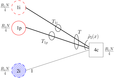
Figure 14: Part of the compact graph representation of the Tanner graph of a root-LDPC for coded cooperation. The number of edges connecting ($1i$, $1p$) to $4c$ is $T$. the number of edges connecting $1p$ to $4c$ is $T_{1p}$. The number of edges connecting $1i$ to $4c$ is $T_{1i}$.

$$T \stackrel{{\scriptstyle a)}}{{=}} \frac{R_{1}N/4}{\sum_{i}\tilde{\rho}_{2i}/i}$$ (31)

$$T_{1p} \stackrel{{\scriptstyle a)}}{{=}} \frac{R_{1}N/4}{\sum_{i}\lambda_{i}/i}$$ (32)

$$T_{1i} \stackrel{{\scriptstyle a)}}{{=}} \frac{R_{1}N/4}{\sum_{i}\tilde{\lambda}_{i}/i}$$ (33)

$$f_{1p4c} \stackrel{{\scriptstyle b)}}{{=}} \frac{T_{1p}}{T}$$ (34)

$$f_{1i4c} \stackrel{{\scriptstyle b)}}{{=}} \frac{T_{1i}}{T}.$$ (35)

a)

The number of checknodes connected to $i$ edges of $T$ is $\frac{\tilde{\rho}_{2i}}{i}T$. A Similar reasoning proves equations (32) and (33).

b)

The fraction of edges $T$ connecting $1p$ to $4c$ is $f_{1p4c}$. The fraction of edges $T$ connecting $1i$ to $4c$ is $f_{1i4c}$.

∎

The DE equations in the neighborhood of $1p$ and $p_{1}^{\prime}$ for a $(\lambda_{1}(x),\rho_{1}(x),\lambda_{2}(x),\rho_{2}(x))$ RCR-LDPC ensemble for coded cooperation can be derived similarly.

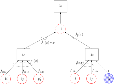
Figure 15: Local neighborhood of bitnode $1i$. This tree is used to determine the evolution of the density of messages $1i\rightarrow 3c$.

Figure 16: Local neighborhood of bitnode $1i$. This tree is used to determine the evolution of the density of messages $1i\rightarrow 4c$.

Proposition 5 can be used for multiple purposes. First of all, it is used to estimate the asymptotic performance. For a fixed fading set $(\alpha_{12},\alpha_{21},\alpha_{1d},\alpha_{2d})$, it is possible to determine whether the bit error probability converges to $0$ or not. We refer to the event where the bit error probability does not converge to $0$ by Density Evolution Outage ($DEO$). Thus, at a fixed SNR, it is possible to determine the probability of a Density Evolution Outage $P_{DEO}$ by averaging over a sufficient number of fading instances. Now, it is possible to write the word error probability $P_{ew}$ of the ensemble as

$$P_{ew}=P_{ew|DEO}\times P_{DEO}+P_{ew|CONV}\times(1-P_{DEO});$$ (36)

where $P_{ew|DEO}$ is the word error probability given a DEO event, $P_{ew|DEO}=1$, and $P_{ew|CONV}$ is the word error probability when DE converges. The probability $P_{ew|CONV}$ depends on the speed of convergence of density evolution and the population expansion of the ensemble with the number of decoding iterations [24], so that

$$P_{DEO}\leq P_{ew}.$$ (37)

Thus, the performance estimated via density evolution is a lower bound for the word error probability.

Secondly, Proposition 5 can be used to determine the threshold of $\mathcal{C}$ on an ergodic channel. This does not directly serve the performance analysis for the BF channel. However, an analysis in the real space of the fading coefficients has shown that this can be used to increase the coding gain on a BF relay channel [12]. But the optimization of the coding gain is outside the scope of this paper and here we will only use Proposition 5 in the application of Eq. (37).

VI Numerical Results

In this section we estimate the asymptotic performance of RCR-LDPC codes through DE and verify Eq. (37) through finite length simulations. We studied different scenarios:

VI-1 Scenario 1

• The average SNR of the independent interuser channels is 5dB higher than the average SNR on the source-destination link.

• The average SNR of the relay-destination link is equal to that on the source-destination link.

• The coding rate is $R_{c}=\frac{1}{3}$ and the cooperation level is $\beta=0.5$.

For this scenario, we have tested two code ensembles: a regular (3,9,3,6) RCR-LDPC code and an irregular $(\lambda_{1}(x),\rho_{1}(x),\lambda_{2}(x),\rho_{2}(x))$ RCR-LDPC code with left and right degree distributions given by the polynomials

$$\lambda_{1}(x) = 0.1989x+0.2305x^{2}+0.0068x^{5}+0.2774x^{6}$$

$$+0.14267x^{19}+0.1335x^{20}+0.0102x^{21},$$

$$\rho_{1}(x) = x^{12},$$

$$\lambda_{2}(x) = 0.22767x+0.20333x^{2}+0.2145x^{5}$$

$$+0.011048x^{6}+0.34346x^{19},$$

$$\rho_{2}(x) = 0.5x^{7}+0.5x^{8}.$$

VI-2 Scenario 2

• The average SNR of the independent interuser channels is 12dB higher than the average SNR on the source-destination link.

• The average SNR of the relay-destination link is 4dB higher than the average SNR on the source-destination link.

• The coding rate is $R_{c}=0.45$ and the cooperation level is $\beta=0.5$.

Here, we imitated the channel conditions used in [20]. The average SNR of the interuser channels is high with respect to the uplink channels, allowing a high coding-rate for the source-relay channel. We used an irregular $(\lambda_{1}(x),\rho_{1}(x),\lambda_{2}(x),\rho_{2}(x))$ RCR-LDPC ensemble with left and right degree distributions given by the polynomials

$$\lambda_{1}(x) = 0.1581x+0.2648x^{2}+0.1116x^{5}+0.1354x^{6}$$

$$+0.3301x^{14},$$

$$\rho_{1}(x) = x^{43},$$

$$\lambda_{2}(x) = 0.234413x+0.21392x^{2}+0.123711x^{5}+0.125548x^{6}$$

$$+0.30241x^{19},$$

$$\rho_{2}(x) = 0.71875x^{7}+0.28125x^{8}.$$

The coding rate for the interuser channel subcode $H_{1}$ is equal to $0.9$.

VI-A Density Evolution Outage

We evaluated the asymptotic performance of RCR-LDPC codes by applying DE on the proposed code construction. The probability of Density Evolution Outage $P_{DEO}$, which is a lower bound of the WER, for both scenarios is illustrated in Fig. 17.

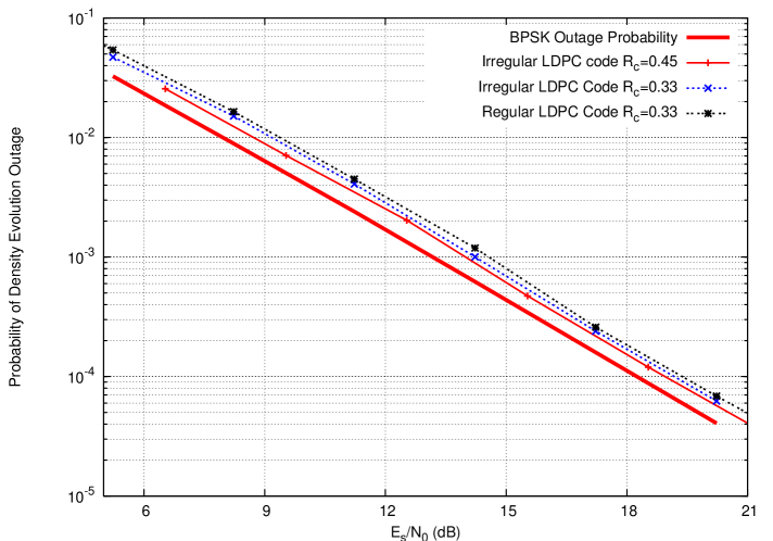
Figure 17: Density Evolution Outage probability of RCR-LDPC codes with coding rates $R_{c}=\frac{1}{3}$ (scenario 1) and $R_{c}=0.45$ (scenario 2) with iterative decoding on a cooperative MAC with two users. $E_{s}/N_{0}$ is the average symbol energy-to-noise ratio on the source-destination link.

Note that the outage probability for both rates is, by coincidence, too close to distinguish. The simulated RCR-LDPC code ensembles all perform within $1.5\textrm{dB}$ from the outage probability limit, whereas the irregular RCR-LDPC code ensembles are within $1\textrm{dB}$ from the outage probability limit. This distance is respected for many variations of the channel conditions, such as other interuser channel conditions or uplink channel conditions. Note that our code construction can be applied on a full-duplex channel, doubling the overall spectral efficiency. As mentioned before, the coding rate is adjustable by varying the number of parity bits $p_{1}^{\prime}$ and $p_{2}^{\prime}$, which is illustrated in scenario 2.

In this work, we mainly focussed on the diversity order achieved by the code construction. In more recent work [12] we optimized the degree distribution using the analysis of Section V. Another method is based on density evolution with a modified Gaussian approximation that takes into account the SNR variation in one received codeword as well as the rate-compatibility constraint [28].

VI-B Finite Length LDPC Codes

It is interesting to evaluate the finite length performance of the proposed RCR-LDPC codes. Not only to approve the asymptotic performance, but also to see how to generate an instance of the parity-check matrix, given by Fig. 8. Before showing the results, we will first discuss the practical generation of this parity-check matrix.

Consider case 1 from Fig. 2. For the decoding process, the destination will apply the sum-product algorithm on the overall graph including $H_{1s}$, $H_{1r}$, and $H_{2}$. For the encoding process, it is easier to determine the parity bits $p_{1}^{\prime}$, $p_{2}^{\prime}$, and $(1p,2p)$ with the parity-check matrices $H_{1s}$, $H_{1r}$, and $H_{2}$ respectively. As with standard LDPC encoding, these matrices will then be systemized to determine the parity bits. An important constraint for the decoding process is the alignment in the overall parity-check matrix of common bit nodes in both constituent codes. This can be achieved by prohibiting column permutations during the systemization of $H_{1s}$, $H_{1r}$ and $H_{2}$. Except for case 4, which only decodes on $H_{1s}$, the other cases need the same constraints.

VI-B1 Generation of $H_{1s}$ and $H_{1r}$

$H_{1s}$ and $H_{1r}$ are randomly generated satisfying the degree distribution $\rho_{1}(x)$ for its rows and the degree distribution $\lambda_{1}(x)$ for its columns. A sufficient condition to prohibit column permutations during the systemization of $H_{1s}$ and $H_{1r}$ is imposing on $H_{p_{1}^{\prime}}$ and $H_{p_{2}^{\prime}}$ to be full-rank. $H_{p_{1}^{\prime}}$ ($H_{p_{2}^{\prime}}$ respectively) is the most right square matrix of $H_{1s}$ ($H_{1r}$ respectively).

VI-B2 Generation of $H_{2}$

The generation of $H_{2}$ can be split in the generation of $H_{4c}$ and $H_{3c}$, where $H_{3c}$ ($H_{4c}$ resp.) is the upper part (resp. lower part) of the parity-check matrix $H_{2}$. $H_{3c}$ is the concatenation of an identity matrix (permutation matrix), zeros and a randomly generated matrix $(H_{2i},H_{2p})$. The rows of $(H_{2i},H_{2p})$ satisfy the degree distribution $\tilde{\rho}_{2}(x)$, the columns of the most left square matrix $H_{2i}$ satisfy the degree distribution $\tilde{\lambda}_{2}(x)$ and the columns of the most right square matrix $H_{2p}$ satisfy the degree distribution $\lambda_{2}(x)$. This is equivalent to generating a random graph with two classes of bitnodes at the left side and one class of checknodes at the right side of the graph. If $n_{3c}$ is the number of checknodes at the right side, then a random graph with $\frac{n_{3c}}{\sum_{i}\tilde{\rho}_{2i}}$ edges is generated. A fraction $\frac{\sum_{i}\tilde{\rho}_{2i}/i}{\sum_{i}\tilde{\lambda}_{2i}/i}$ of the edges is connected to bit nodes of the class $2i$, whereas a fraction $\frac{\sum_{i}\tilde{\rho}_{2i}/i}{\sum_{i}\lambda_{2i}/i}$ of the edges is connected to bit nodes of the class $2p$. In the end, the identity matrix is simply added. $H_{4c}$ is generated similarly.
For the encoding process, we have to systemize this matrix. One solution is to switch the columns associated with the $1i$ bit node class and the $2p$ bit node class. The most left square matrix of $H_{2}$ will then be block-diagonal with $H_{2p}$ and $H_{1p}$ on its diagonal. Having $H_{2p}$ and $H_{1p}$ full-rank is consequently a sufficient condition to exclude column permutations during the systemization of this matrix. After the generation of $(2p,1p)$, all the bits are put in the required order $1i-1p-2i-2p$ by switching back the bits of the classes $1i$ and $1p$.

VI-B3 WER performance of finite length LDPC codes

The probability of Density Evolution Outage $P_{DEO}$ is a lower bound of the WER of LDPC ensembles without cycles in its Tanner graph, which is illustrated in Fig. 18 for irregular codes and in Fig. 19 for the regular code of scenario 1. In the latter, we augment the blocklength to show that the WER of LDPC codes is independent of the block length. The results shows that inequality (37) is very tight in this case.

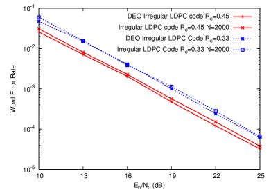
Figure 18: Comparison of Density Evolution Outage (DEO) probability of irregular RCR-LDPC codes with coding rates $R_{c}=\frac{1}{3}$ (scenario 1) and $R_{c}=0.45$ (scenario 2) with iterative decoding on a cooperative MAC with two users. $E_{b}/N_{0}$ is the average information bit energy-to-noise ratio on the source-destination link.

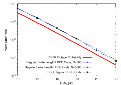
Figure 19: Comparison of RCR-LDPC codes for different block lengths with iterative decoding on a cooperative MAC for two users, coding rate $R_{c}=1/3$. The ratio $E_{b}/N_{0}$ is the average information bit energy-to-noise ratio on the source-destination link.

VI-C Comparison with Previous Work

As mentioned in the introduction, especially rate-compatible punctured convolutional codes (RCPC) have been used in coded cooperation. The main drawback of these codes is that the WER increases with the logarithm of the block length to the power $d$ where $d$ is the diversity order [6], [7], whereas the WER of near-outage codes should be independent of the block length. This can be seen clearly on Fig. 20, where we show the WER of two rate-compatible non-recursive non-systematic (75,53,47) convolutional codes with block length 500 and 5000 respectively. We used the same channel conditions and coding rate as in scenario 1.

We also compared with another protocol, Decode and Forward (DF), using near-outage LDPC codes for this protocol. Despite the fact that this implementation has near-outage performance, the WER performance is worse than that of our code construction. The reason is that the outage probability limit of DF is higher than that of coded cooperation.

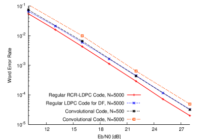
Figure 20: Comparison of RCR-LDPC codes for coded cooperation with other work on a cooperative MAC for two users. We simulated LDPC codes for Decode and Forward under iterative decoding and an implementation of rate-compatible convolutional codes [21]. The ratio $E_{b}/N_{0}$ is the average information bit energy-to-noise ratio on the source-destination link.

VI-D Comparison with fully random LDPC codes

Finally, a comparison with random LDPC codes is made. In Sec. IV-B, the global parity-check matrix is obtained by embedding the root-LDPC matrix (Fig. 7) into the rate-compatible matrix (Fig. 3). When using codes that are fully random generated, i.e., no special rootchecks are used, then the global parity-check matrix is obtained by embedding a random LDPC matrix into the rate-compatible matrix (Fig. 3), see Fig. 21, where $H_{1}$ and $H_{2}$ are randomly generated.

Figure 21: Parity-check matrix of a rate-compatible LDPC code obtained by the extension of higher rate codes. Symbols are split into three classes: $i$ for the information bits, $1p$ and $2p$ for two classes of parity bits. The classes $i$ and $1p$ are transmitted by the source in frame 1. Parity bits $2p$ are transmitted in the second frame, for example by the relay after successful decoding of the first frame. Matrix $H_{1}$ is used to protect the information bits on the source channel. The parity bits generated by the relay provide an extra protection through the code $H_{2}$.

We simulated the same scenarios from the previous subsections, using the same code for $H_{1}$ and using the degree distribution of previously published excellent LDPC codes for the Gaussian channel for the random generation of $H_{2}$.

VI-D1 Scenario 1

$$\lambda_{2}(x) = 0.189x+0.177x^{2}+0.136x^{4}+0.126x^{5}+0.027x^{6}$$

$$+0.037x^{11}+0.006x^{13}+0.076x^{21}+0.225x^{28},$$

$$\rho_{2}(x) = 0.153x^{4}+0.125x^{5}+0.040x^{6}+0.261x^{7}$$

$$+0.149x^{8}+0.178x^{9}+0.041x^{10}+0.055x^{11},$$

where the coding rate of $(\lambda_{2}(x),\rho_{2}(x))$ is $R_{c2}=0.4$, so that the overall coding rate is $R_{c}=1/3$. The comparison with a regular $(3,9,3,6)$ RCR-LDPC code is shown in Fig. 22.

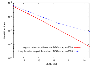
Figure 22: Comparison of RCR-LDPC codes with rate-compatible random LDPC codes for coded cooperation on a cooperative MAC for two users, coding rate $R_{c}=1/3$. The ratio $E_{b}/N_{0}$ is the average information bit energy-to-noise ratio on the source-destation link.

VI-D2 Scenario 2

$$\lambda_{2}(x) = 0.230x+0.164x^{2}+0.149x^{5}+0.126x^{6}+0.027x^{7}$$

$$+0.037x^{15}+0.006x^{16}+0.243x^{17}+0.018x^{23},$$

$$\rho_{2}(x) = 0.153x^{5}+0.425x^{7}+0.149x^{8}+0.273x^{9},$$

where the coding rate of $(\lambda_{2}(x),\rho_{2}(x))$ is $R_{c2}=9/19$, so that the overall coding rate is $R_{c}=0.45$. The comparison with an irregular RCR-LDPC code is shown in Fig. 23.

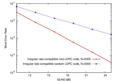
Figure 23: Comparison of RCR-LDPC codes with rate-compatible random LDPC codes for coded cooperation on a cooperative MAC for two users, coding rate $R_{c}=0.45$. The ratio $E_{b}/N_{0}$ is the average information bit energy-to-noise ratio on the source-destination link.

In scenario 1, the threshold of $(\lambda_{2}(x),\rho_{2}(x))$ is $E_{b}/N_{0}=0.1$dB which is $0.338$dB from the Shannon limit; and in scenario 2, the threshold of $(\lambda_{2}(x),\rho_{2}(x))$ is $E_{b}/N_{0}=0.4$dB which is $0.33$dB from the Shannon limit. Despite the excellent thresholds of the codes in both scenarios, full-diversity is not achieved. From these two examples, it is clear that rootchecks are necessary to have full-diversity.

VII Conclusion

We have studied LDPC codes for relay channels in a slowly varying fading environment under iterative decoding. We have introduced the new family of rate-compatible root-LDPC codes, which combines the rate-compatibility property with the full-diversity property for any coding rate $R_{c}\leq R_{cmax}=\textrm{min}(\beta,1-\beta)$, where $\beta$ is the cooperation level. Through a density evolution analysis and finite length simulations, we have shown that the error rate performance of regular and irregular rate-compatible root-LDPC codes is close to the outage probability limit and this occurs for all block lengths (finite and infinite) and all rates not exceeding $R_{cmax}$. Its flexibility and high performance makes rate-compatible root-LDPC attractive for wireless cooperative communications scenarios with slowly varying fading.

Dieter Duyck (S’09) received the M.S. degree in electrical engineering in 2007 from the Katholieke Universiteit Leuven (KUL), Leuven, Belgium. In 2006, he spent one year with the Communications and Electronics Department, at the Ecole Nationale Supérieure des Télécommunications (ENST, Telecom ParisTech), Paris, France. In 2007, he started his Ph.D. research at the Department of Telecommunications and Information Processing (TELIN), Ghent University, Gent, Belgium.

From Oct. 2007 until present, he conducted his Ph.D. research. He has held visiting appointments with Ecole Nationale Supérieure des Télécommunications (ENST), Paris, France; and Texas A&M University at Qatar, Doha, Qatar. His research interests are in communication theory, information theory, channel coding, joint network-channel coding, digital modulation and space-time coding.

M. Sc. Dieter Duyck received the first Young Researcher Award for [13] awarded by the Award Committee, formed by all Advisory Board Members of the European Newcom++ (Network of Excellence in Wireless COMmunications). He also received the best student paper award at the IEEE Symposium on Communications and Vehicular Technology in the Benelux (SCVT) in 2010.

Joseph Jean Boutros (M’94, SM’09) received the M.S. degree in electrical engineering in 1992 and the Ph.D. degree in 1996, both from Ecole Nationale Supérieure des Télécommunications (ENST, Telecom ParisTech), Paris, France. From 1996 to 2006, he was with the Communications and Electronics Department, ENST, as an Associate Professor. He was also a member of the research unit UMR-5141 of the French National Scientific Research Center (CNRS). In 2007, he joined Texas A&M University at Qatar (TAMUQ) as a full Professor in the electrical engineering program. He has been a scientific consultant for Alcatel Espace, Philips Research, and Motorola Semiconductors, and was a member of the Digital Signal Processing team of Juniper Networks Cable. His fields of interest are codes on graphs, iterative decoding, joint source-channel coding, space-time coding, and lattice sphere packings.

Marc Moeneclaey (M’93, SM’99, F’02) received the diploma of electrical engineering and the Ph.D. degree in electrical engineering from Ghent University, Gent, Belgium, in 1978 and 1983, respectively.

He is Professor at the Department of Telecommunications and Information Processing (TELIN), Gent University. His main research interests are in statistical communication theory, (iterative) estimation an detection, carrier and symbol synchronization, bandwidth-efficient modulation and coding, spread-spectrum, satellite and mobile communication. He is the author of more than 400 scientific papers in international journals and conference proceedings. Together with Prof. H. Meyr (RWTH Aachen) and Dr. S. Fechtel (Siemens AG), he co-authors the book Digital communication receivers Synchronization, channel estimation, and signal processing. (J. Wiley, 1998). He is co-recipient of the Mannesmann Innovations Prize 2000.

During the period 1992-1994, he was Editor for Synchronization, for the IEEE Transactions on Communications. He served as co-guest editor for special issues of the Wireless Personal Communications Journal (on Equalization and Synchronization in Wireless Communications) and the IEEE Journal on Selected Areas in Communications (on Signal Synchronization in Digital Transmission Systems) in 1998 and 2001, respectively.

References

- [1] K. Azarian, H. El Gamal, and P. Schniter, “On the achievable diversity-multiplexing tradeoff in half-duplex cooperative channels,” IEEE Trans. Inf. Theory, vol. 51, no. 12, pp. 4152-4172, Dec. 2005.
- [2] X. Bao and J. Li, “Decode-amplify-forward (DAF): a new class of forwarding strategy for wireless relay channels,” Proc. IEEE SPAWC, New York, pp. 816-820, June 2005.
- [3] E. Biglieri, J. Proakis, S. Shamai, “Fading channels: information-theoretic and communications aspects,” IEEE Trans. Inf. Theory, vol. 44, no. 6, pp. 2619-2692, Oct. 1998.
- [4] E. Biglieri, Coding for wireless channels, New York, Springer-Verlag, 2005.
- [5] J.J. Boutros, A. Guillén i Fàbregas, E. Biglieri, and G. Zémor, “Design and Analysis of Low-Density Parity-check Codes for Block-Fading Channels,” IEEE Information Theory and Applications Workshop, pp. 54-62, Jan. 2007, DOI: 10.1109/ITA.2007.4357562.
- [6] J.J. Boutros, E. Calvanese, and A. Guillén i Fàbregas, “Turbo code design for block fading channels,” Allerton Conf. on Communication and Control, Illinois, 2004.
- [7] J.J. Boutros, A. Guillén i Fàbregas, and E. Calvanese, “Analysis of coding on non-ergodic block fading channels,” Allerton Conf. on Communication and Control, Illinois, 2005.
- [8] J.J. Boutros, A. Guillén i Fàbregas, E. Biglieri, and G. Zémor, “Low-Density Parity-check Codes for Nonergodic Block-Fading Channels,” IEEE Trans. Inf. Theory, vol. 56, no. 9, pp. 4286-4300, Sep. 2010, DOI: 10.1109/TIT.2010.2053890.
- [9] A. Chakrabarti, A. de Baynast, A. Sabharwal, and B. Aazhang, “Low-density parity-check codes for the relay channel,” IEEE journal on selected areas in communications, vol. 25, no. 2, Feb. 2007.
- [10] T.M. Cover and J.A. Thomas, Elements of Information Theory, New York, Wiley, 2006.
- [11] T. Cover and A.E. Gamal, “Capacity theorems for the relay channel,” IEEE Trans. Inf. Theory, vol. IT-25, no. 5, pp. 572-584, Sep. 1979.
- [12] D. Duyck, M. Azmi, J. Yuan, J.J. Boutros, M. Moeneclaey, “Universal LDPC codes for Cooperative Communications,” Turbo Code Symposium, Brest, France, Sep. 2010.
- [13] D. Duyck, D. Capirone, J.J. Boutros, and M. Moeneclaey, “A full-diversity joint network-channel code construction for cooperative communications,” Personal Indoor Mobile Radio Communications (PIMRC), Tokyo, Japan, Sept. 2009.
- [14] D. Duyck, D. Capirone, J.J. Boutros, and M. Moeneclaey, “Analysis and construction of full-diversity joint network-LDPC codes for cooperative communications,” Eur. Journal on Wireless Comm. and Netw., vol. 2010, Article ID 805216, 16 pages, 2010.
- [15] D. Duyck, D. Capirone, M. Heindlmaier, and M. Moeneclaey, “Towards full-diversity joint network-channel coding for large networks,” European Wireless Conference (EWC), Vienna, Austria, April 2011.
- [16] A. Guillén i Fàbregas, Concatenated codes for block-fading channels, Ph.D. thesis, EPFL, June 2004.
- [17] A. Guillén i Fàbregas, and G. Caire, “Coded modulation in the block-fading channel: coding theorems and code construction,” IEEE Trans. Inf. Theory, vol. 52, no. 1, pp. 91-114, Jan. 2006.
- [18] J. Ha, J. Kim, and S.W. McLaughlin, “Rate-Compatible Puncturing of Low-Density Parity-check Codes,” IEEE Trans. Inf. Theory, vol. 50, no. 11, pp. 2824-2836, Nov. 2004.
- [19] J. Hagenauer, “Rate-compatible punctured convolutional codes (RCPC codes) and their applications,” IEEE Trans. Commun., vol. 36, no. 4, pp. 389-400, Apr. 1988, DOI: 10.1109/26.2763.
- [20] J. Hu and T.M. Duman, “Low Density Parity Check Codes over Wireless Relay Channels,” IEEE Trans. Wireless Commun., vol. 6, no. 9, pp. 3384-3394, Sep. 2007, DOI: 10.1109/TWC.2007.06083.
- [21] T.E. Hunter, Coded cooperation: a new framework for user cooperation in wireless systems, Ph.D. thesis, University of Texas at Dallas, 2004.
- [22] A. Nosratinia and T.E. Hunter, “Diversity through coded cooperation,” IEEE Trans. Wireless Commun., vol. 5, no. 2, pp. 283-289, Feb. 2006, DOI: 10.1109/TWC.2006.1611050.
- [23] T.E. Hunter, S. Sanayei, and A. Nosratinia, “Outage analysis of coded cooperation,” IEEE Trans. Inf. Theory, vol. 52, no. 2, pp. 375-391, Feb. 2006.
- [24] H. Jin and T. Richardson, “Block error iterative decoding capacity for LDPC codes,” IEEE International Symp. on Inf. Theory, Adelaide, Sep. 2005.
- [25] R. Knopp and P.A. Humblet, “On coding for block fading channels,” IEEE Trans. Inf. Theory, vol. 46, no. 1, pp. 189-205, Jan. 2000.
- [26] J.N. Laneman, D. Tse, and G.W. Wornell, “Cooperative diversity in wireless networks: Efficient protocols and outage behavior,” IEEE Trans. Inf. Theory, vol. 50, no. 12, pp. 3062-3080, Dec. 2004.
- [27] A. Lapidoth, “The performance of convolutional codes on the block erasure channel using various finite interleaving techniques,” IEEE Trans. Inf. Theory, vol. 40, no. 5, pp. 1459-1473, Sep. 1994, DOI: 10.1109/18.333861.
- [28] C. Li, G. Yue, X. Wang, and M.A. Khojastepour, “LDPC Code Design for Half-duplex Cooperative Relay,” IEEE Trans. on Wireless Commun., vol. 7, no. 11, pp. 4558-4567, Nov. 2008, DOI: 10.1109/T-WC.2008.070482.
- [29] J. Li and K. Narayanan, “Rate-compatible low density parity check codes for capacity-approaching ARQ scheme in packet data communications,” Proc. Int. Conf. Commun. Internet Inf. Technol., pp. 201-206, Nov. 2002.
- [30] E. Malkamäki and H. Leib, “Evaluating the performance of convolutional codes over block fading channels,” IEEE Trans. Inf. Theory, vol. 45, no. 5, pp. 1643-1646, Jul. 1999.
- [31] E.C. van der Meulen, “Three-Terminal Communication Channels,” Adv. Appl. Prob., vol. 3, no. 1, pp. 120-154, 1971.
- [32] A. Nosratinia, T.E. Hunter, and A. Hedayat, “Cooperative communication in wireless networks,” IEEE Commun. Mag., vol. 42, no. 10, pp. 74-80, Oct. 2004.
- [33] L.H. Ozarow, S. Shamai and A.D. Wyner, “Information theoretic considerations for cellular mobile radio,” IEEE Trans. Veh. Technol., vol. 43, no. 2, pp. 359-379, May 1994, DOI: 10.1109/25.293655.
- [34] P. Razaghi and W. Yu, “Bilayer Low-Density Parity-Check Codes for Decode-and-Forward in Relay Channels,” IEEE Trans. Inf. Theory, vol. 53, no. 10, pp. 3723-3739, Oct. 2007, DOI: 10.1109/TIT.2007.904983.
- [35] P. Razaghi and W. Yu, “Bit-Interleaved Coded Modulation for the Relay Channel Using Bilayer LDPC Codes,” 10th Canadian Workshop on Information Theory, Edmonton, Alberta, Canada, June 6-8, 2007.
- [36] T.J. Richardson and R.L. Urbanke, “The capacity of low-density parity-check codes under message-passing decoding,” IEEE Trans. Inf. Theory, vol. 47, no. 2, pp. 599-618, Feb. 2001.
- [37] T.J. Richardson and R.L. Urbanke, Modern Coding Theory, Cambridge Univ. Press, Cambridge, U.K., 2008.
- [38] T.J. Richardson, M.A. Shokrollahi, and R.L. Urbanke, “Design of capacity-approaching irregular low-density parity-check codes,” IEEE Trans. Inf. Theory, vol. 47, no. 2, pp. 619-637, Feb. 2001.
- [39] T.J. Richardson and R.L. Urbanke, “Multi-Edge Type LDPC Codes,” IEEE Trans. Inf. Theory, submitted 2004.
- [40] A. Sendonaris, E. Erkip, and B. Aazhang, “User cooperation diversity-Part I: System description,” IEEE Trans. Commun., vol. 51, no. 11, pp. 1927-1938, Nov. 2003, DOI: 10.1109/TCOMM.2003.818096.
- [41] A. Sendonaris, E. Erkip, and B. Aazhang, “User cooperation diversity-Part II: Implementation aspects and performance analysis,” IEEE Trans. Commun., vol. 51, no. 11, pp. 1939-1948, Nov. 2003.
- [42] J. Thorpe, “Low-Density Parity-Check (LDPC) codes constructed from protographs,” JPL INP Progress Report, vol. 42-154, pp. 1-7, Aug. 2003.
- [43] D.N.C. Tse and P. Viswanath, Fundamentals of Wireless Communication, Cambridge Univ. Press, Cambridge, U.K., May 2005.
- [44] G. Ungerboeck, “Channel coding with multilevel/phase signals,” IEEE Trans. Inf. Theory, vol. IT-28, no. 1, pp. 55-67, 1982.
- [45] M. Yazdani and A.H. Banihashemi, “Irregular rate-compatible LDPC codes for capacity-approaching hybrid-ARQ schemes,” Canadian Conf. on Electrical and Computer Engineering, 2004.
- [46] B. Zhao and M.C. Valenti, “Some new adaptive protocols for the wireless relay channel,” Allerton conference on communication control and computing, vol. 41, no. 3, pp. 1588-1589, 2003.