Accretion and diffusion in white dwarfs

Abstract

Context. A number of cool white dwarfs with metal traces, of spectral types DAZ, DBZ, and DZ have been found to exhibit infrared excess radiation due to circumstellar dust. The origin of this dust is possibly a tidally disrupted asteroid that formed a debris disk now supplying the matter accreting onto the white dwarf. To reach any clear conclusions from the observed composition of the white dwarf atmosphere to that of the circumstellar matter, we need a detailed understanding of the accretion and diffusion process, in particular the diffusion timescales.

Aims. We aim to provide data for a wide range of white dwarf parameters and all possible observed chemical elements.

Methods. Starting from atmosphere models, we calculate the structure of the outer envelopes, obtaining the depth of the convection zone and the physical parameters at the lower boundary. These parameters are used to calculate the diffusion velocities using calculations of diffusion coefficients available in the literature.

Results. With a simple example, we demonstrate that the observed element abundances are not identical to the accreted abundances. Reliable conclusions are possible only if we know or can assume that the star has reached a steady state between accretion and diffusion. In this case, most element abundances differ only by factors in the range 2-4 between atmospheric values and the circumstellar matter. Knowing the diffusion timescales, we can also accurately relate the accreted abundances to the observed ones. If accretion has stopped, or if the rates vary by large amounts, we cannot determine the composition of the accreted matter with any certainty.

1 Introduction

Heavy elements in cool white dwarfs ($\la 25\,000$ K) should diffuse downward in the atmospheres due to gravitational settling in the high gravitational fields (Schatzman, 1945). Nevertheless, one of the first three “classical” white dwarfs, van Maanen 2, has been found to exhibit strong Ca ii resonance lines. This star has a helium-rich atmosphere and is the prototype of the spectral class DZ. Although an example of a star containing a hydrogen-rich atmosphere with metal traces, G 74-7, had been known for a considerable period of time (see the analysis by Billeres et al., 1997), it was not until 1997, that DAZ was finally established as an important class (Koester et al., 1997; Holberg et al., 1997), although DA are the dominant spectral type of white dwarfs. The reason for the delay was observational bias. Because of the much higher opacity of hydrogen at low temperatures around 6000-20000 K, metal spectral lines are far weaker in a hydrogen atmosphere at the same abundances. Large telescopes were therefore needed to detect DAZs in significant numbers (Zuckerman & Reid, 1998; Zuckerman et al., 2003; Koester et al., 2005).

Since diffusion timescales are always short compared to evolution timescales, the metals must be supplied from a source from outside, with the possible exception of carbon in the DQs, which can be dredged-up from deeper layers (Koester et al., 1982). Assuming the interstellar matter to be the outer source, this so-called accretion/diffusion scenario was discussed in great detail in three fundamental papers by Dupuis et al. (1992, 1993a, 1993b). However, there are some severe problems with this scenario: the apparent lack or at least significant underabundance of hydrogen in the accreted matter, and the lack of any correlation between the location of the white dwarfs and the conditions of the ISM. Alternative scenarios were therefore discussed, such as the accretion of comets (Alcock et al., 1986), or a tidally disrupted asteroid (Jura, 2003). A thorough discussion of these alternative models was given by Zuckerman et al. (2003).

These objects have become the subject of renewed interest following the detection of infrared excess radiation indicative of the presence of circumstellar dust (Zuckerman & Becklin, 1987; Becklin et al., 2005; Kilic et al., 2005, 2006; von Hippel et al., 2007; Jura et al., 2007). Although the spectra from optical to IR can be fairly well modeled with simple disk models (e.g., Jura et al., 2007), the exact geometrical distribution was only confirmed with the detection of gaseous metal disks around hotter white dwarfs, which clearly show the signature of Keplerian rotation (Gänsicke et al., 2006).

For all stars exhibiting metal traces in their atmospheres and infrared excesses due to circumstellar dust, the source of the current accretion is obviously the matter surrounding the star. The most plausible origin – and the only one discussed in the current literature – is an asteroid remaining from a former planetary system, which has been tidally disrupted by the white dwarf. If metals are found in the atmosphere, but no infrared excess, the situation is unclear. However, Jura (2008) argues that in such a case the circumstellar material may be provided by a higher number of small asteroids instead of a single large one.

One should not forget, however, that the accretion process is not well understood. We are not aware of a study of accretion from the ISM for realistic conditions in the solar neighborhood, with a mixture of gas and dust, and different phases of the ISM, but observationally we know that on all scales in the universe, accretion is always accompanied by the formation of an accretion disk. We should therefore not exclude from our current considerations the possibility of some kind of compromise between the current two models, accretion from the ISM and accretion from the debris disk of a former asteroid.

It is widely accepted that accretion from the ISM occurs for almost all white dwarfs during their lifetimes because more than half of all DB (and with higher quality observations perhaps all) show traces of hydrogen, which according to our current understanding can only be accreted (Voss et al., 2007). This is also true for the significant amount of hydrogen detected in GD 362. If the accreted metals indeed originate in a disrupted asteroid, one has to assume an independent source for the hydrogen, unless the asteroid contained a substantial amount of water (Jura et al., 2009). The approximately solar ratio of metals to hydrogen (see below) is in both scenarios purely accidental.

An important tool in understanding the origin of this dust is the determination of its composition by the analysis of the atmospheric abundances. The latter is straightforward (if high-resolution, high signal-to-noise spectra can be obtained!), but the connection between atmospheric and accreted composition requires a detailed understanding of the accretion and diffusion processes. The composition of the accreting matter need not necessarily be identical to that of the circumstellar matter (see e.g., Alcock & Illarionov, 1980). And the composition observed in the stellar atmosphere is modified by diffusion out of the outer reservoir, which occurs at different rates (diffusion timescales) for different elements. This is the part of the problem studied in this paper, which extends the work of Koester & Wilken (2006).

Since the study of Koester & Wilken (2006), infrared excess radiation has been identified in many more hydrogen-rich and helium-rich white dwarfs with metals. Improved observations have allowed us to identify 15 heavy elements and place upper limits on a few more in GD 362 (Zuckerman et al., 2007). For many of those elements, diffusion timescales are unavailable in the literature, inhibiting any firm conclusions about the composition of the circumstellar matter. We therefore calculated atmosphere and envelope models for hydrogen and helium atmosphere white dwarfs throughout the interesting temperature range and calculated the timescales for many elements. In this work, we follow the ground work laid by the Montreal group, using their data on the Coulomb collision integrals (Paquette et al., 1986a) and to a large extent the methods outlined in Paquette et al. (1986b).

2 Envelope models

To determine diffusion timescales, we need to model the structure of the outer layers of the white dwarfs, including the complete convection zone. The outer boundary is determined from atmospheric models, which assume Local Thermodynamic Equilibrium (LTE), hydrostatic equilibrium, convective energy transport, and a detailed calculation of the radiative energy transfer. An up-to-date description of input physics, data, and numerical methods is given by Koester (2009). The parameters of these models are effective temperature $T_{\mathrm{eff}}$ and surface gravity $\log g$, in addition to the element abundances. The models are calculated down into the star to very large Rosseland optical depth $\tau_{\mathrm{R}}$, usually between 1000 and 1500.

The value of physical parameters such as pressure, temperature, and density, at some defined value $\tau_{\mathrm{R}}$, which is a free parameter chosen to be between 1 and 500, is the starting point for the integration of the deeper layers. In this integration, we also need to know the mass and radius of the star, which were obtained from the finite temperature mass-radius relations of Wood (1995).

We use the standard equations of stellar structure for the conservation of mass, hydrostatic equilibrium, and energy transfer. The fourth equation, of energy conservation, is replaced by the assumption that the energy flux $l(r)$ at the radius $r$ is proportional to the mass $m(r)$ inside that radius

$$l(r)=\frac{L}{M}\,m(r),$$ (1)

for total mass $M$ and luminosity $L$. This is almost equivalent to assuming a constant luminosity throughout the outer layers. The equations are integrated inward from the boundary condition until the fractional mass in the envelope $\Delta M/M=(1-m(r)/M)$ reaches approximately $10^{-4}$. The algorithms and variable definitions, as well as the program code, are taken in large part from our white dwarf structure code, which has been used in numerous projects. Updated input physics included in our code, are the following:

• the equation of state (EOS) is that of Saumon et al. (1995), which is adapted from the tables obtained from the AAS CD-ROM series Vol. 5 (1995). This is probably the most sophisticated EOS for hydrogen/helium mixtures available today.

• absorption coefficients were obtained from the OPAL project (Iglesias & Rogers, 1996), supplemented at low temperatures with the tables of Ferguson et al. (2005).

• thermal conductivity data are from Potekhin et al. (1999); the tables were obtained from their website.

The OPAL tables were slightly extended at high densities by data calculated for H/He mixtures with the help of the Los Alamos TOPS program on their web-site. Nevertheless, in some of our envelope models, the structure falls into a regime of the opacity tables, where the assumptions become invalid and the data are unreliable. In this case, the highest reliable density value at the given temperature was used in the extrapolation. Fortunately this had no effect, since in this regime the opacity is always high and the models are convective, the temperature gradient being practically adiabatic. We confirmed this finding by using instead old Los Alamos opacity tables (Cox & Stewart, 1970), and no significant changes to the models were found.

2.1 The convection zone

The convection zone in white dwarfs – both the atmosphere and envelope – is calculated with a version of the mixing-length approximation. It has become customary to denote the specific version as, e.g., ML2/$\alpha=0.6$ or in shorthand as ML2/0.6. Here ML2 represents a choice of three dimensionless parameters, which are defined and explained in Fontaine et al. (1981) and Tassoul et al. (1990), the number (0.6) is the mixing-length as a multiple of the pressure scale height. Koester et al. (1994) and Bergeron et al. (1995) demonstrated that a version with “intermediate” efficiency of energy transport is the best choice for DAs in ensuring a consistent fit to optical and UV spectra simultaneously. The Bergeron choice ML2/0.6 is the de-facto standard for DA model atmospheres today, and our “standard” grid in this paper also uses this version in atmosphere and envelope calculations.

To our knowledge there is no comparable published study of DB white dwarfs. However, there is in Beauchamp et al. (1999) a reference to spectroscopic fits of optical and UV data, which favors the version ML2/1.25. We note that these conclusions for DAs and DBs are based on observed spectra and thus describe the atmospheric layers, which produce the emerging light, i.e., above $\tau_{\mathrm{R}}\approx 1$.

It is well established that the deeper layers of the atmosphere and envelope are not necessarily correctly described by the same version of the mixing-length approximation. The atmospheric parameters of G 29-38 are $T_{\mathrm{eff}}$ = 11 700 K, $\log g$ = 8.10, when analyzed with ML2/0.6 models. The convection zone in such a model is extremely thin, and has a lower boundary at around optical depth 10. Such a thin cvz has a thermal timescale, defined as

$$\tau_{\mathrm{th}}=\frac{\int_{0}^{M_{\mathrm{cvz}}}c_{P}Tdm}{L}$$ (2)

of less than 1s. However, G 29-38 is a variable ZZ Ceti star, with a shortest period a little larger than 200s. Winget et al. (1983) and Tassoul et al. (1990) argued that the thermal timescale of the cvz should be similar to the period, that is the cvz should be much deeper than indicated by the atmospheric ML parameters. The same conclusion is reached by fitting the non-linear light-curve; the thermal timescale at 11 700 K is predicted to be $\approx 100$s (Montgomery, 2005).

From a completely different point of view, a similar conclusion was reached by Ludwig et al. (1994). By comparing the mean temperature structure in two-dimensional hydrodynamic simulations of the outer layers of a DA white dwarf with model atmospheres using MLT, they found that no single MLT version can describe the entire structure of the cvz. The efficiency, or in the MLT parameterization the mixing-length, must increase with depth.

We therefore calculated a second set of DA envelopes, where the MLT version was switched to ML2/2.0 in the envelope calculation. The result depends strongly on the exact structure of the atmosphere model and the location of the “matching point”, the starting point in the envelope integration. If this layer is below the atmospheric cvz, e.g., deeper than $\tau_{\mathrm{R}}\approx 10$ in the case of the G29-38 model, or at such large depth that the convection is nearly adiabatic, the envelope integration will not produce any deepening of the cvz, regardless of the efficiency of the MLT version. The matching must occur within the super-adiabatic part of the atmospheric convection zone for the change in efficiency to influence the model structure. We considered the optical depth of this layer as a free parameter and calibrated it by demanding a thermal timescale of $\approx 100$s for the G29-38 model. This is of course unsatisfactory, and in the future we hope to find a more consistent description with a smooth change of efficiency from shallow to deeper layers. Nevertheless, our choice is supported by the pulsation properties of the DAs and should provide more realistic estimates of diffusion timescales.

The situation is more favorable for the DB stars than for the DAs. Benvenuto & Althaus (1997) compared results for thermal timescales and cvz depths in DBs between the more sophisticated convection theory of Canuto & Mazzitelli (1991, 1992) and Canuto et al. (1996), with different simple MLT versions. They concluded that a convective efficiency between ML2/1.0 and ML2/2.0 reproduces the results and predicts the correct location of the blue edge of the DB instability strip. This was confirmed by Córsico et al. (2008), who concluded that only ML2/1.25 predicts the correct location. A similar result was also obtained from the light-curve fitting of the prototype variable DB star GD 358 (Montgomery, 2007). We thus chose this version for both the atmosphere and the envelope calculations.

More fundamentally, it is well known that the MLT approximation provides a poor description of the various aspects of a real convection zone. For the case of DA white dwarfs, this was studied with an extensive comparison of two-dimensional radiation-hydrodynamic simulations with 1D structures by Freytag et al. (1996). Even the definition of the lower boundary is ambiguous: depending on whether one uses the classical stability criterion, the layers with significant convective flux, or the layers with non-zero velocities, the resulting mass in the “convection zone” can differ by orders of magnitude. While the temperature structure (related to convective flux) is probably the most important quantity for the pulsational properties, for diffusion timescales, the mixed region with non-zero velocity is relevant. In the example studied by Freytag et al. (1996), the mass in the latter is 300 times higher than in the former.

The general result that the velocity field extends far below the lower limit of the unstable region and even the flux overshoot was also confirmed by Montgomery & Kupka (2004) with their non-local model of convection in DAs. This implies that the diffusion timescales in stars with convection zones may be orders of magnitude larger than estimated with our current MLT approximations.

Table 1: Conditions at the bottom of the convection zones in DA models with surface gravity $\log g=8$ and the standard mixing length version ML2/0.6 for atmosphere and envelope. The second column is the fractional mass $q=\log M_{\mathrm{cvz}}/M$ in the zone or down to an optical depth $\tau_{R}=5$, whichever is deeper. The next columns give the logarithms of gas pressure, temperature, and mass density at this level. All physical quantities are in cgs units.

$T_{\mathrm{eff}}$	$\log M_{\mathrm{cvz}}/M$	$\log P$	$\log T$	$\log\rho$
6000.	-7.570	14.510	5.914	0.393
7000.	-8.423	13.655	5.758	-0.293
8000.	-9.002	13.076	5.665	-0.773
9000.	-9.719	12.359	5.543	-1.371
9500.	-10.278	11.799	5.438	-1.826
10000.	-11.063	11.014	5.289	-2.466
10500.	-12.094	9.983	5.098	-3.310
11000.	-13.392	8.684	4.870	-4.386
11100.	-13.681	8.395	4.821	-4.629
11200.	-13.975	8.101	4.771	-4.876
11300.	-14.288	7.788	4.718	-5.136
11400.	-14.638	7.438	4.653	-5.422
11500.	-15.049	7.026	4.559	-5.739
11600.	-15.427	6.649	4.456	-6.013
11700.	-15.675	6.401	4.393	-6.196
11800.	-15.850	6.225	4.353	-6.330
11900.	-15.947	6.129	4.332	-6.404
12000.	-16.006	6.070	4.321	-6.450
12500.	-16.065	6.010	4.316	-6.504
13000.	-16.070	6.006	4.326	-6.521
14000.	-16.009	6.067	4.361	-6.500
15000.	-15.949	6.126	4.391	-6.472
16000.	-15.891	6.185	4.420	-6.444
17000.	-15.839	6.237	4.447	-6.420
18000.	-15.794	6.282	4.473	-6.400
19000.	-15.754	6.322	4.496	-6.385
20000.	-15.719	6.357	4.518	-6.371
21000.	-15.687	6.389	4.538	-6.361
22000.	-15.658	6.417	4.558	-6.351
23000.	-15.632	6.444	4.575	-6.343
24000.	-15.607	6.469	4.592	-6.335
25000.	-15.584	6.492	4.609	-6.328

Table 2: Similar to Table 1, but with a more efficient convective energy transport in the deeper layers, as explained in the text. For $T_{\mathrm{eff}}$ $>$ 13000 K the entries are identical with Table 1 and are not repeated here.

$T_{\mathrm{eff}}$	$\log M_{\mathrm{cvz}}/M$	$\log P$	$\log T$	$\log\rho$
6000.	-7.564	14.516	5.916	0.398
7000.	-8.376	13.703	5.769	-0.256
8000.	-8.876	13.202	5.691	-0.673
9000.	-9.429	12.649	5.602	-1.140
9500.	-9.803	12.275	5.536	-1.448
10000.	-10.328	11.749	5.437	-1.877
10500.	-11.040	11.037	5.303	-2.457
11000.	-11.945	10.132	5.135	-3.198
11100.	-12.151	9.926	5.097	-3.367
11200.	-12.364	9.712	5.058	-3.543
11300.	-12.587	9.490	5.019	-3.727
11400.	-12.819	9.258	4.978	-3.919
11500.	-13.058	9.018	4.936	-4.118
11600.	-13.301	8.775	4.895	-4.320
11700.	-13.544	8.532	4.853	-4.522
11800.	-13.806	8.270	4.809	-4.743
11900.	-13.996	8.080	4.777	-4.902
12000.	-14.229	7.847	4.738	-5.097
12500.	-15.555	6.521	4.437	-6.122
13000.	-16.070	6.006	4.326	-6.521

Table 3: Similar to Table 1, but for DB white dwarfs. Convection parameters are ML2/1.25 for atmosphere and envelope models.

$T_{\mathrm{eff}}$	$\log M_{\mathrm{cvz}}/M$	$\log P$	$\log T$	$\log\rho$
6000.	-4.840	17.243	5.938	2.868
7000.	-4.754	17.330	6.098	2.909
8000.	-4.760	17.324	6.275	2.882
9000.	-4.789	17.296	6.440	2.825
10000.	-4.833	17.253	6.551	2.754
11000.	-4.954	17.131	6.598	2.636
12000.	-5.132	16.954	6.603	2.486
13000.	-5.332	16.752	6.589	2.322
14000.	-5.545	16.538	6.565	2.151
15000.	-5.780	16.303	6.532	1.964
16000.	-6.059	16.023	6.486	1.743
17000.	-6.413	15.668	6.421	1.462
18000.	-6.884	15.196	6.331	1.086
19000.	-7.572	14.507	6.202	0.531
20000.	-8.657	13.421	5.992	-0.333
21000.	-10.046	12.031	5.727	-1.470
22000.	-11.368	10.708	5.493	-2.567
23000.	-11.581	10.495	5.463	-2.751
24000.	-11.746	10.330	5.441	-2.895
25000.	-11.911	10.165	5.419	-3.038

3 Diffusion coefficients and timescales

For the calculation of diffusion timescales we follow closely the fundamental works of Paquette et al. (1986a) and Paquette et al. (1986b). From the tables in the first paper, we take the fit coefficients for the calculation of Coulomb collision integrals and the diffusion coefficients as well as thermal diffusion coefficients. The equations to calculate diffusion velocities are taken from the second paper with two minor modifications. First, we use what the authors call the “second method” for the thermal diffusion coefficient. This is based on the approach by Chapman & Cowling (1970), and the necessary data can be found in the first paper cited above. The second change is purely cosmetic. To determine the effective charge of the trace element 2, we calculate an effective ionization potential $\chi_{\mathrm{eff}}$ as described in their Eqs. 19-21, and compare this with the true ionization potentials $\chi(Z)$ of the ions of element 2 with charge $Z$. Rather than taking the effective charge as $Z$, if $\chi_{\mathrm{eff}}(Z)/\chi(Z)\leq 1$ and $\chi_{\mathrm{eff}}(Z+1)/\chi(Z+1)>1$, we interpolate a non-integer $Z_{\mathrm{eff}}$ between $Z$ and $Z+1$. Diffusion coefficients and diffusion velocities are then calculated for ions $Z$ and $Z+1$ and a weighted average taken depending on the value of $Z_{\mathrm{eff}}$. The only purpose of this approach is to avoid unphysical wiggles and steps in the relation between diffusion timescales and effective temperatures (see e.g., Fig. 4 in Paquette et al. (1986b)).

The diffusion velocity $v_{\mathrm{diff}}$ is obtained using Eq. 4 in Paquette et al. (1986b), neglecting the concentration term, since we consider only diffusion of trace elements. The diffusion time scale is

$$\tau_{\mathrm{diff}}=\frac{M_{\mathrm{cvz}}}{4\pi r^{2}\,\rho\,v_{\mathrm{diff}}}$$ (3)

where $r$ is the local radius at the bottom of the convection zone and $\rho$ is the local mass density. Results for the stellar models in Tables 1 to 3 are given in Tables 4 to 6 for six important elements; data for other models and/or other elements can be requested from the author.

Table 4: Diffusion timescales at the base of the convection zone (or at $\tau_{\mathrm{R}}=5$) for DA models with $\log g$ = 8, using the standard assumption of ML2/0.6 for atmosphere and envelope models. Columns 2-6 give the logarithm of the timescales in years for the elements C, Na, Mg, Si, Ca, and Fe.

$T_{\mathrm{eff}}$	C	Na	Mg	Si	Ca	Fe
6000.0	4.50	4.34	4.29	4.21	4.14	4.00
7000.0	3.88	3.60	3.54	3.52	3.45	3.33
8000.0	3.49	3.16	3.07	3.12	3.06	2.95
9000.0	3.03	2.70	2.60	2.66	2.61	2.50
9500.0	2.68	2.31	2.21	2.30	2.24	2.13
10000.0	2.18	1.74	1.65	1.79	1.68	1.59
10500.0	1.55	0.98	0.95	1.15	0.94	0.88
11000.0	0.55	-0.00	0.05	0.32	-0.04	-0.03
11100.0	0.33	-0.22	-0.13	0.14	-0.25	-0.24
11200.0	0.10	-0.46	-0.33	-0.07	-0.46	-0.44
11300.0	-0.14	-0.72	-0.55	-0.33	-0.69	-0.67
11400.0	-0.41	-1.01	-0.79	-0.61	-0.94	-0.92
11500.0	-0.74	-1.35	-1.07	-0.98	-1.25	-1.22
11600.0	-1.03	-1.64	-1.32	-1.31	-1.51	-1.57
11700.0	-1.35	-1.84	-1.50	-1.52	-1.70	-1.80
11800.0	-1.54	-1.97	-1.63	-1.66	-1.83	-1.95
11900.0	-1.65	-2.05	-1.70	-1.74	-1.90	-2.04
12000.0	-1.70	-2.10	-1.74	-1.79	-1.95	-2.09
12500.0	-1.74	-2.14	-1.78	-1.83	-1.99	-2.12
13000.0	-1.73	-2.14	-1.79	-1.83	-1.99	-2.12
14000.0	-1.61	-2.08	-1.73	-1.76	-1.93	-2.04
15000.0	-1.48	-2.03	-1.69	-1.70	-1.89	-1.97
16000.0	-1.36	-1.98	-1.65	-1.64	-1.84	-1.90
17000.0	-1.32	-1.94	-1.62	-1.58	-1.80	-1.83
18000.0	-1.28	-1.90	-1.59	-1.53	-1.77	-1.77
19000.0	-1.24	-1.86	-1.57	-1.48	-1.74	-1.71
20000.0	-1.21	-1.83	-1.55	-1.43	-1.72	-1.68
21000.0	-1.18	-1.80	-1.53	-1.38	-1.69	-1.66
22000.0	-1.15	-1.77	-1.51	-1.34	-1.67	-1.64
23000.0	-1.12	-1.74	-1.50	-1.31	-1.65	-1.61
24000.0	-1.09	-1.70	-1.48	-1.27	-1.63	-1.59
25000.0	-1.06	-1.67	-1.47	-1.24	-1.60	-1.57

Table 5: Similar to Table 4, but with more efficient convection (ML2/2.0) below $\tau_{\mathrm{R}}=2$, leading to deeper convection zones in closer agreement with expectations for the variable ZZ Cetis.

$T_{\mathrm{eff}}$	C	Na	Mg	Si	Ca	Fe
6000.0	4.50	4.34	4.29	4.21	4.15	4.01
7000.0	3.91	3.64	3.58	3.55	3.49	3.37
8000.0	3.57	3.25	3.16	3.20	3.14	3.03
9000.0	3.22	2.91	2.81	2.85	2.82	2.70
9500.0	2.98	2.67	2.56	2.61	2.57	2.46
10000.0	2.65	2.30	2.20	2.27	2.22	2.11
10500.0	2.19	1.78	1.68	1.81	1.72	1.62
11000.0	1.64	1.12	1.05	1.24	1.07	0.99
11100.0	1.51	0.95	0.91	1.11	0.92	0.85
11200.0	1.37	0.79	0.77	0.98	0.75	0.70
11300.0	1.19	0.61	0.61	0.84	0.58	0.54
11400.0	1.00	0.43	0.45	0.69	0.39	0.38
11500.0	0.82	0.25	0.29	0.54	0.22	0.22
11600.0	0.64	0.07	0.12	0.38	0.03	0.04
11700.0	0.45	-0.10	-0.03	0.23	-0.14	-0.13
11800.0	0.25	-0.30	-0.21	0.06	-0.33	-0.31
11900.0	0.10	-0.46	-0.34	-0.07	-0.47	-0.45
12000.0	-0.08	-0.66	-0.50	-0.26	-0.64	-0.62
12500.0	-1.15	-1.74	-1.42	-1.41	-1.61	-1.68
13000.0	-1.73	-2.14	-1.79	-1.83	-1.99	-2.12

Table 6: Similar to Table 4, but for non-DA models without outer hydrogen layer (DB, DC).

$T_{\mathrm{eff}}$	C	Na	Mg	Si	Ca	Fe
6000.0	6.50	6.57	6.55	6.59	6.56	6.56
7000.0	6.48	6.52	6.54	6.52	6.53	6.49
8000.0	6.40	6.40	6.41	6.40	6.41	6.33
9000.0	6.34	6.32	6.32	6.32	6.32	6.22
10000.0	6.31	6.28	6.28	6.29	6.27	6.15
11000.0	6.25	6.21	6.22	6.20	6.18	6.06
12000.0	6.17	6.13	6.13	6.09	6.05	5.94
13000.0	6.06	6.01	5.98	5.96	5.88	5.80
14000.0	5.96	5.88	5.85	5.85	5.72	5.64
15000.0	5.84	5.72	5.71	5.71	5.53	5.46
16000.0	5.68	5.54	5.54	5.49	5.33	5.24
17000.0	5.51	5.35	5.32	5.23	5.11	4.98
18000.0	5.26	5.05	4.99	4.89	4.83	4.64
19000.0	4.73	4.62	4.56	4.44	4.43	4.22
20000.0	4.06	3.99	3.91	3.77	3.78	3.56
21000.0	3.22	3.12	3.00	2.86	2.96	2.68
22000.0	2.36	2.15	2.05	1.89	2.03	1.82
23000.0	2.21	2.00	1.90	1.74	1.89	1.67
24000.0	2.07	1.85	1.75	1.60	1.75	1.53
25000.0	1.90	1.66	1.57	1.42	1.57	1.37

4 Elementary considerations for the accretion/diffusion scenario

The possibility of this scenario providing an explanation of the observed metals in cool white dwarfs was studied extensively in a series of three papers by Dupuis and collaborators (Dupuis et al., 1992, 1993a, 1993b). In the first two of those papers, the authors solved the complete problem of time-dependent accretion and diffusion, by considering the spatial and temporal distribution of a heavy element during the white dwarf cooling evolution. They also showed that for trace elements in the outer convection zone – which is always homogeneously mixed – the computation can be replaced by a much simpler local calculation at the bottom of the convection zone. We use this approximation here to derive some basic consequences of debris disk accretion onto white dwarfs, which are not always appreciated in the current literature.

The basic equation for the mass abundance $X_{\mathrm{cvz}}(el)$ of heavy element $el$ in the convection zone becomes (see Eq. 1 in Dupuis et al., 1992, with slightly different notation)

$$M_{\mathrm{cvz}}\,\frac{dX_{\mathrm{cvz}}(el,t)}{dt} = \dot{M}(el)-4\pi r^{2}\,X_{\mathrm{cvz}}(el,t)\,\rho\,v(el)$$ (4)

$$= \dot{M}(el)-\frac{X_{\mathrm{cvz}}(el,t)\,M_{\mathrm{cvz}}}{\tau_{\mathrm{diff}}}$$

where the first term on the right side is the accretion rate of that element, and the second term is the rate of gravitational settling (where we use a positive velocity to represent elements diffusing downward). Assuming that $\tau,\dot{M},v$ are constant, the solution of this equation is

$$X_{\mathrm{cvz}}(el,t)=X_{\mathrm{cvz}}(el,0)\,{\mathrm{e}}^{-t/\tau(el)}+\frac{\tau(el)\,\dot{M}(el)}{M_{\mathrm{cvz}}}\,\left[1-{\mathrm{e}}^{-t/\tau(el)}\right]$$ (5)

where the first term on the right side is the starting value of the element abundance at the beginning of the accretion phase.

Some conclusions can be drawn immediately from this simple equation. If the accretion rate is constant for some multiple of the diffusion timescale ($\approx 5$ for practical purposes, given the typical uncertainties in observed elemental abundances), the abundance will approach an asymptotic (“steady state”) value (we omit the index $\mathrm{cvz}$ from $X$ for simplicity) of

$$X(el,\infty)=\frac{\tau(el)\,\dot{M}(el)}{M_{\mathrm{cvz}}}$$ (6)

and for the ratio of elements 1 and 2, we obtain

$$\frac{X(el1)}{X(el2)}=\frac{\tau(el1)\,\dot{M}(el1)}{\tau(el2)\,\dot{M}(el2)}=\frac{\tau(el1)}{\tau(el2)}\,\frac{X_{\mathrm{acc}}(el1)}{X_{\mathrm{acc}}(el2)},$$ (7)

where in the last step, we replaced the accretion rate by the element abundances in the accreted matter. If the diffusion times are less than a few years, we can reasonably assume that this steady state has been reached. Since we can calculate the timescales from the parameters of the star, we can thus determine the abundances in the accreted matter from the observed abundances in the star. Even more simply, since the timescales for the commonly observed elements of Ca, Mg, and Fe are often within a factor of two, we can assume the observed abundances (which are rarely more accurate than a factor of 2) to be a first approximation to the accreted abundances.

However, all of these conclusions depend critically on the assumption that the steady state is reached, and are therefore valid only in the case of short diffusion timescales. It is instructive to consider by a simple example, the consequences of being unable to assume steady state (i.e., in all cases where the timescales exceed a few years).

For this exercise, we studied the abundances of two elements, where the diffusion timescales differed by a factor of two. We started with zero abundance and switched accretion on for 10 times the shorter timescale. Then accretion is switched off again.

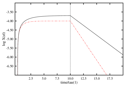
Figure 1: Simple example for the accretion/diffusion scenario with two elements.

We were able to distinguish three phases (see Fig. 1)

1. for $t\ll\tau_{1},\tau_{2}$, expansion of the exponentials in the equation above shows that the diffusion timescales cancel; the element abundances increase linearly with time, with the slope given by the accretion rates (or the abundances in the accreted matter)

2. for $t\approx\tau$, the abundances approach the steady state values, which are reached after $\approx 5\tau$. In this phase, the abundances of the accreted material are modified by the ratio of the diffusion timescales, which is here equal to 2

3. when the accretion is switched off, the abundances decrease exponentially. Because of the difference in diffusion timescales, the ratio also increases exponentially and can reach very large values – in this simple case $>100$ after 10 diffusion timescales. At this point, the element abundances are only 2-4 orders of magnitude below their maximum values, which would be observable in many cases.

The third phase would also describe a different scenario, where accretion occurs at a high rate in a short time, such as the accretion of an entire asteroid at once. The abundances would reflect exactly the accreted abundances during this time and start the exponential decay from there. In such a case we would be unable able to determine the composition of the accreted matter.

We note that the above example is not extreme. In particular, when including light or very heavy elements in the comparison the factor between timescales can be $\approx 4$. And we also do not need to consider the extreme case of totally switching accretion on and off. Even a change in the accretion rate, for example by a factor of 100 leads to an intermediate change in the abundance ratio of a factor $>10$, before the asymptotic ratio of 2 is reached again.

The conclusion of this simple exercise is that it is only possible to infer abundances of the accreted matter if we can safely assume that the accretion rate has been constant for several times the diffusion timescales of all elements involved, and that therefore the steady state has been reached. For diffusion timescales longer than a few decades at most this can never be assumed. Equating the observed atmospheric abundance ratios to those of the accreted matter can in such cases be incorrect by orders of magnitude.

5 Specific examples

We apply the general results to two specific objects with circumstellar material and atmospheric metal traces, which have been discussed in numerous recent studies: G 29-38 and GD 362.

5.1 G 29-38

Based on three independent determinations (Liebert et al., 2005; Koester et al., 1997; Voss, 2006), we use the atmospheric parameters $T_{\mathrm{eff}}$ = 11 690 K, $\log g$ = 8.11. An atmosphere/envelope model was calculated with these data and Table 7 collects the diffusion timescales and observed abundances from Koester et al. (1997) and Zuckerman et al. (2003). Unfortunately, there is some confusion about the Ca abundance in the literature – even using only studies with contributions from this author. The reason is that the Vienna Atomic Line Database (VALD) contains Stark broadening data for the Ca ii H and K resonance lines, which differ by about a factor of 10 from most of the Kurucz lists. Depending on which data are used, the abundance differs by about 0.5 dex. Using simple estimates for Stark broadening indicates that the larger broadening constants are more likely correct and thus the lower Ca abundance is preferred.

For the model, we used the version with the more efficient convection, which provides a reasonable thermal timescale of about 100 s. Since the diffusion timescales are still smaller than one year, the conclusions are not qualitatively changed compared to the standard version, which was used in Koester & Wilken (2006). There is a significant caveat, however: as discussed in a previous section, even though the thermal timescale agrees with the pulsation properties, the possible overshooting at the bottom might increase the diffusion timescales significantly. Another effect in the same direction is the pulsation itself. During the pulsational decrease in the effective temperature (up to 500 K; Montgomery, 2005), the depth of the convection zone increases significantly, leading to a larger mixed zone and an increase in the diffusion timescale by almost a factor of 10 compared to the equilibrium model.

Metals were first detected in G 29-38 in 1997 (Koester et al., 1997). Von Hippel & Thompson (2007) claimed changes had occurred in the equivalent width of the Ca ii resonance lines during the past decade, which was questioned by Debes & López-Morales (2008). We have seven high-quality high-resolution spectra from the ESO VLT and the Keck telescope, which show no significant variation between 1997 and 2000; the von Hippel & Thompson (2007) result may have been influenced by the inhomogeneity of their data, which included time-resolved spectroscopy of very low S/N.

Table 7: Diffusion data for the variable ZZ Ceti star G 29-38. Column 2 gives the time scale in years, column 3 the observed number abundances relative to Ca, column 4 the observed abundances by mass, also relative to Ca. Column 5 is the predicted abundance in the accreting material, assuming steady state between accretion and diffusion. The final column shows the solar abundances on the same scale. All abundances are in decadal logarithms.

el	$\tau$ [yrs]	$\log\epsilon_{\mathrm{atm}}$	$\log X_{\mathrm{atm}}$	$\log X_{\mathrm{acc}}$	$\log X_{\odot}$
Ca	0.79	0.00	0.00	0.00	0.00
Mg	0.97	1.10	0.88	0.79	1.00
Fe	0.80	0.61	0.82	0.81	1.33

In view of the short diffusion timescales, it seems thus reasonable to assume that this object at the moment is experiencing steady state accretion. Because of the similar timescales, the predicted accretion abundances do not differ too much from the observed values. Taking into account that there is a factor of 3 difference in the Mg abundance between Koester et al. (1997) and Zuckerman et al. (2003) and a similar uncertainty in the Fe abundance (high vs. low dispersion spectra, optical vs. UV spectra), we can conclude that within the rather large uncertainties, the abundances of Ca, Fe, and Mg in the accreted matter are compatible with solar abundances, taken from the compilation in Astrophysical Quantities (Cox, 2000).

5.2 GD 362

GD 362 was discovered as a massive DA with metals (DAZ) by Gianninas et al. (2004). An infrared excess (Kilic et al., 2005) placed it into the new class of DA white dwarfs with debris disks. However, an analysis of high S/N, high-resolution spectra (Zuckerman et al., 2007, Z07 henceforth) showed it to be a normal mass, but helium-rich object. We used the stellar parameters for an atmosphere/envelope model, and inferred the diffusion parameters in Table 8. We found that the fractional mass in the convection zone is $q=-6.58$, and, using the mass 0.73 M_⊙ from Z07, that the total hydrogen mass in the envelope is $3.51\times 10^{-9}$ M_⊙, and the total mass of Si is $3.90\times 10^{21}$ g. The combined mass of the clearly identified elements Mg, Al, Si, Ca, Fe, and Ni is $\approx 1.8\times 10^{22}$ g, in excellent agreement with the estimates in Z07.

Table 8: Diffusion data for GD 362. The meaning of the columns is the same as in Table 7, except that all element abundances are presented relative to Si.

el	$\tau$ [yrs]	$\log\epsilon_{\mathrm{atm}}$	$\log X_{\mathrm{atm}}$	$\log X_{\mathrm{acc}}$	$\log X_{\odot}$
C	1.28 $10^{5}$	$<$0.20	$<$-0.17	$<$-0.38	0.64
N	1.22 $10^{5}$	$<$1.70	$<$1.39	$<$ 1.20	0.20
O	1.13 $10^{5}$	$<$0.70	$<$0.45	$<$ 0.30	1.14
Na	9.50 $10^{4}$	-1.95	-2.04	-2.11	-1.33
Mg	9.44 $10^{4}$	-0.14	-0.21	-0.28	-0.04
Al	8.57 $10^{4}$	-0.56	-0.60	-0.63	-1.10
Si	7.95 $10^{4}$	0.00	0.00	0.00	0.00
Ca	6.07 $10^{4}$	-0.40	-0.25	-0.13	-1.04
Sc	5.83 $10^{4}$	-4.35	-4.15	-4.02	-4.24
Ti	5.45 $10^{4}$	-2.11	-1.88	-1.72	-2.33
V	5.20 $10^{4}$	-2.90	-2.64	-2.46	-3.29
Cr	5.05 $10^{4}$	-1.57	-1.31	-1.11	-1.61
Mn	4.77 $10^{4}$	-1.63	-1.34	-1.12	-1.87
Fe	4.67 $10^{4}$	0.19	0.49	0.72	0.29
Co	4.43 $10^{4}$	-2.66	-2.34	-2.09	-2.31
Ni	4.45 $10^{4}$	-1.23	-0.91	-0.66	-0.98
Cu	4.25 $10^{4}$	-3.34	-2.99	-2.72	-2.98
Sr	3.14 $10^{4}$	-4.58	-4.09	-3.69	-4.15

Given that the individual abundances vary over more than four orders of magnitude, it is remarkable, how close the inferred accretion abundances (column 5) are to the solar abundance ratios. The error for Si was given as 0.3 dex in Z07, and for the other elements, it ranges from 0.1 to 0.4 dex. The only elements with abundances that differ significantly from the solar value are C and O, for which only upper limits are known, and Ca and Na. Since 12 of 14 elements have a ratio of their abundance to that of Si higher than for solar values might imply that the Si abundance in Z07 is slightly too low, producing a systematic shift.

The possible “abundance history” of GD 362 is shown in Fig. 2, which is in a similar spirit as Fig. 1. We use the elements C, Mg, Si, Ca, Fe, and Sr as representatives for different diffusion timescales and abundances. Accretion is switched on at time $t=0$, when no heavy elements are present in the atmosphere; the rate – the same for all elements – is calculated to ensure a steady state abundance of silicon of $\log X(\mathrm{Si})=-5$, the observed value. The silicon rate necessary for this is $2.4\times 10^{17}$ g per year. A different rate would shift all curves vertically by the same amount. In reality, the elements would of course be accreted with different abundances. In our choice of presentation, the difference between the curves shows directly the relative change between the accreted and atmospheric abundance ratios. When all the curves are approximately in agreement, the observed abundance ratios are identical to the accreted ratios. In this specific case, this is true for times $t\la 3\times 10^{4}$ yrs. After that time, the steady state is approached, and the ratio differs from the accreted ones by the ratios of the diffusion timescales, which are factors of 2-4 in this case.

After the accretion is switched off, the picture changes significantly. About $4\times 10^{5}$ yrs after the end of accretion, the ratios can differ from the accreted abundance ratios by factors of up to 200. This decline is fast on astronomical timescales, but slow enough to be invisible over a few decades; we thus do not have any direct indication of the phase we are currently observing. It should also be noted – as in the simple example above – that a change in the accretion rate of a factor of 10-100 would force the star into a phase of exponential decline, until a new steady state with lower abundances was reached.

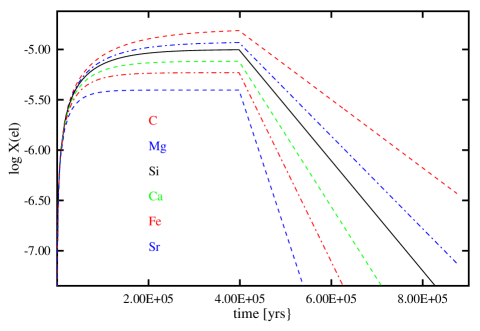
Figure 2: Possible accretion/diffusion history for GD 362. The element symbols are ordered in the same sequence as the corresponding curve.

In their study of accretion from the interstellar matter, Dupuis et al. (1993a) assumed schematically a duration of the accretion phase within a dense ISM cloud of $10^{6}$ yrs. This would correspond to the time required to complete all of the process indicated in Fig.2, and all phases would be possible for the current situation. On the other hand, in the scenario of accretion from the debris disk formed by an asteroid (see e.g., Z07 for an extensive discussion), the total accreted matter of the identified elements alone would be $\approx 7.5\times 10^{23}$ g after $3\times 10^{5}$ yrs, close to the mass of Ceres, the most massive asteroid in our system. This agrees with estimates of the lifetime of the debris disks, which are of the order of $1.5\times 10^{5}$ yrs (Jura, 2008; Kilic et al., 2008).

It is thus highly likely that we are witnessing the early phase of accretion, and that it will be possible to identify the composition of the accreted matter. This view is further supported by the visibility of rare elements such as strontium, which have short diffusion timescales. Within $\approx 10^{5}$ yrs of the end of the accretion phase, the Sr abundance would decrease by an order of magnitude, becoming undetectable.

We also note that the aforementioned deviations from solar abundances for C, N, Na, and Ca cannot be explained by assuming a post-accretion phase. Deviations would be in the opposite direction of expectations: C, O, and Na are underabundant, but should increase in this phase, and vice versa for Ca.

An element of particular importance for the accretion/diffusion scenario is hydrogen, because as the lightest element, it will always remain in the convection zone and not diffuse downward. Assuming that hydrogen would be accreted with solar ratio with respect to silicon, the current hydrogen mass present – $6.98\times 10^{24}$ g – would be reached in 16 580 yrs. We either are observing GD 362 in the very early phase of accretion, or the accreted matter is significantly hydrogen-depleted.

Jura et al. (2009) considered an exponentially decreasing accretion rate, which would be appropriate if the dust disk is not replenished from a reservoir farther out in the system. In such a case, the diffusion equation can also be solved analytically to have the solution (in our notation)

$$X_{\mathrm{cvz}}(el,t) = X_{\mathrm{cvz}}(el,0)\,{\mathrm{e}}^{-t/\tau(el)}$$ (8)

$$+ \frac{\tau(el)\,\dot{M}_{0}(el)}{M_{\mathrm{cvz}}}\,\frac{\tau_{\mathrm{acc}}}{\tau_{\mathrm{acc}}-\tau(el)}\,\left[{\mathrm{e}}^{-t/\tau_{\mathrm{acc}}}-{\mathrm{e}}^{-t/\tau(el)}\right]$$

with a timescale for the accretion rate of $\tau_{\mathrm{acc}}$ and an initial rate $\dot{M}_{0}(el)$. We calculated the “abundance history” for GD 362 with the smaller of the two times considered in Jura et al. (2009), $\tau_{\mathrm{acc}}=1.5\times 10^{5}$ yrs, and show the results in Fig. 3.

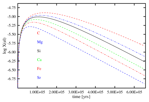
Figure 3: Alternative history for GD 362, assuming an exponentially declining accretion rate. Otherwise the meaning of the curves is the same as in Fig. 2.

In this case, the abundances never reach an asymptotic state, but instead begin to increase, reach a maximum, and then decline. The maxima are reached at different times for the elements, depending on their diffusion timescales. The initial accretion rate for Si (and all other elements) had to be increased by a factor of two from the case of constant rate, because otherwise the Si abundance would never reach the observed value.

In this example, the accretion timescale is longer than all diffusion timescales. As time increases, the later decline is governed by the accretion timescale, which is the same for all elements. The abundance ratios therefore do not show the large deviations from the accreted values as in the case, where accretion is switched off. Instead of the ratios of the diffusion timescales that govern the relative changes in the “steady state”, we obtain here the ratio

$$\frac{X(el1,\infty)}{X(el2,\infty)}=\frac{\tau(el1)\,X_{\mathrm{acc}}(el1)}{\tau(el2)\,X_{\mathrm{acc}}(el2)}\,\frac{\tau_{\mathrm{acc}}-\tau(el2)}{\tau_{\mathrm{acc}}-\tau(el1)},$$ (9)

which for very large $\tau_{\mathrm{acc}}$ relative to $\tau(el)$ recovers the solution for the steady state.

If the accretion timescale is shorter than the diffusion timescale of some elements, then at later times for these elements the conditions approach an exponential decline after the switching off of accretion, and there is the possibility of large deviations from the original abundance. This might in the future be helpful in providing constraints on the lifetimes of the disks.

6 Conclusions

We have extended the calculation of diffusion timescales to many more elements than currently available in the literature, to provide the data necessary to interpret the observed abundances in the increasing number of white dwarfs with traces of metals in their atmospheres and an infrared excess, indicative of the presence of a dust disk. With a simple example and the application to two of the most extensively observed objects (G 29-38 and GD 362), we have demonstrated that the observed abundances are in general not identical to the accreted abundances. If, however, we have good arguments that the steady state between accretion and diffusion is reached, the differences are typically only a factor of 2-4, in many cases within the errors of the determination. This is still true, if the accretion rate changes only slowly, on timescales longer than all diffusion timescales involved. With knowledge of the timescales, we can improve the comparison by calculating the accreted abundances from the observed ones. With further observations of the highest quality, it should thus be possible to resolve the question about the origin of the accreted matter.