Manipulating Higher Partial-Wave Atom-Atom Interaction by Strong Photoassociative Coupling

Abstract

We show that it is possible to change not only s-wave but also higher partial wave atom-atom interactions in cold collision in the presence of relatively intense laser fields tuned near a photoassociative transition.

Ability to control particle-particle interaction is important for exploring quantum physics of many-particle systems in various interaction regimes. Ultracold atoms offer a unique opportunity for such explorations with unprecedented control over atom-atom interaction. There are two methods of manipulating interaction in cold atoms. The most popular one is magnetic field Feshbach resonance (MFR) tiesingaPRA47 which has been extensively used to tune s-wave scattering length over a wide range. This has facilitated the recent demonstration of s-wave fermionic superfluidity in strongly interacting atomic gases Ketterle . In fact, MFR has become an essential tool in experimental investigations on the effects of large s-wave scattering length on the properties of atomic Fermi gases fermi and Bose-Einstein condensates (BEC) bose . The other method of modifying atomic interaction is optical Feshbach resonance (OFR) proposed by Fedichev et al. fedichevPRL771 and implemented in recent experiments fatemiPRL2002 ; theis ; EnomotoPRL101 . While MFR relies on magnetic effects of Zeeman and hyperfine interactions, OFR uses off-resonant continuum-bound optical dipole transitions. In the case of resonance or near-resonance, OFR can lead to photoassociation (PA) parmp of two atoms into an excited molecule. Recently, p-wave MFR ZhangPRA70 in fermionic atoms has been observed. Enhanced scattering in higher partial waves by magnetic-field induced dissociation of Feshabch molecule has been shown rempePRA72 . There is a proposal you for generating anisotropic interaction by static electric field. Both the methods of magnetic and optical Feshbach resonances are so far primarily used to tune s-wave scattering length in ultracold atoms. To go beyond s-wave physics of cold atoms, it is now essential to devise methods of controlling p-, d- and other higher partial-wave interactions. This is particularly important for testing models of unconventional superconductivity or superfluidity in atomic Fermi gases. Superfluidity and superconductivity are related phenomena. Conventional low temperature superconductivity can be explained by Bardeen-Cooper-Schrieffer theory which is based on s-wave Cooper-pairing. It is assumed that higher partial-wave interactions can lead to unconventional and high temperature superconductivity. Studies on Fermi superfluidity in cold atomic gases with controllable p- and d-wave interactions will help us to develop new insight about high temperature superconductivity which requires a proper theoretical understanding.

Here we show that it is possible to change not only $\ell=0$ (s-wave) but also nonzero partial-wave scattering amplitudes of two cold atoms by OFR with a relatively intense laser field. At low energy, the light-shift (or Stark-shift) due to laser-induced free-bound coupling can greatly exceed the spontaneous as well as stimulated line widths of excited molecular state. An intense PA laser can set in two photon processes in which one photon will cause PA transition from continuum to bound level and another photon will induce stimulated transition back to the continuum. If the light-shift largely exceeds the stimulated line width, then even when PA laser is tuned near the unperturbed (without Stark shift) excited molecular level, the formation of excited molecule becomes unlikely due to large light-shift. In such a situation, s-wave scattering wave function can be made to couple to p-wave or even d-wave scattering wave functions depending on the coupling of the molecular axis with the electronic orbital and spin angular momentum. Furthermore, it is possible to enhance $\ell\neq 0$ partial wave scattering amplitudes with multiple strong laser fields causing continuum-bound PA coupling with appropriate rotational states of an excited vibrational level as illustrated in Fig.1.

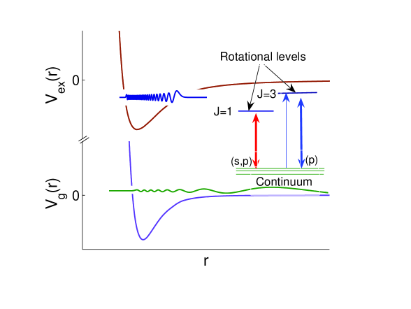
Figure 1: A schematic diagram of ground and excited potentials, scattering and bound states, rotational levels and relevant PA transitions for modifying $\ell\geq 0$ partial wave scattering amplitudes. An intense laser (double arrow red line on the left) is tuned near $J=1$ rotational state (of a particular vibrational level $v$) which can be accessed by PA transitions from s-wave and also at least the next nonzero (p-wave) scattering state. In the strong coupling dispersive regime with large light shift (see text), p-wave scattering amplitude will get modified due to its indirect coupling with s-wave scattering state. This modification can be probed by sending a weak probe laser (single arrow blue line) resonant with $J=3$ PA transition. The modification of p-wave can further be enhanced by applying another intense laser (double arrow blue line on the right) tuned near $J=3$ PA transition.

In this context, recent experimental results EnomotoPRL101 on the intense laser field PA of ytterbium may be of relevance. In molecular bound-bound spectroscopy, it is known that the rotational states of a molecule can be excited by intense laser fields seidmanJCP103 , but exciting higher partial waves in continuum states by continuum-bound PA spectroscopy has not been considered so far.

Let us consider that the scattering state of collision energy $E=\hbar^{2}k^{2}/(2\mu)$ (where $\mu$ is the reduced mass) of two colliding ground state atoms is coupled to an excited molecular state characterized by $v$ vibrational and $J$ rotational quantum numbers. The electronic orbital ($L$) and spin ($S$) angular momentum of the excited diatom are coupled to the diatomic axis according to either Hund’s case (a) or (c). In Hund’s case (a), $\Lambda$ and $\Sigma$ which are the projections of ${\mathbf{L}}$ and ${\mathbf{S}}$, respectively, on the internuclear axis are two good quantum numbers and so is their sum $\Omega=\Lambda+\Sigma$. In Hund’s case (c), the projection $\Omega$ of the total electronic angular momentum $\mathbf{J}_{e}=\mathbf{L}+\mathbf{S}$ is a good quantum number. The angular state of diatom can be written as $\mid J\Omega M\rangle=i^{J}\sqrt{\frac{2J+1}{8\pi^{2}}}{\cal D}^{(J)}_{M\Omega}(\hat{r})$ where $M$ is the z-component of J in the space-fixed coordinate (laboratory) frame. ${\cal D}^{(J)}_{M\Omega}(\hat{r})$ is the rotational matrix element with $\hat{r}$ representing the Euler angles for transformation from body-fixed to space-fixed frame. For $\Omega=0$, ${\cal D}^{(J)}_{M\Omega}(\hat{r})$ reduces to spherical harmonic $Y_{JM}$. The dressed state of a bound level ($v,J$) coupled to a continuum can be written as

$$\Psi_{E} = \sum_{M}\frac{\phi_{vJM}(r)}{r}\mid J\Omega M\rangle\mid e\rangle_{elec}$$ (1)

$$+ \int dE^{\prime}\beta_{E^{\prime}}\sum_{\ell m_{\ell}}\frac{\psi_{E^{\prime}\ell m_{\ell}}(r)}{r}\mid\ell m_{\ell}0\rangle\mid g\rangle_{elec}$$

where $\phi_{vJM}(r)$ is the radial part of the bound state, $\mid\alpha\rangle_{elec}$ denotes internal electronic part of the excited ($\alpha\equiv e$) and ground ($\alpha\equiv g$) molecular states, $\psi_{E^{\prime}\ell m_{\ell}}(r)$ represents energy-normalized partial wave scattering state with collision energy $E^{\prime}$. Here $|\beta_{E^{\prime}}|^{2}$ denotes density of states of the unperturbed continuum. The internal electronic states $\mid\alpha\rangle$ are the functions of electronic coordinates and have parametrical dependence on the internuclear separation $r$. In electric dipole approximation, the interaction Hamiltonian is $H_{int}=\sum_{i=1,2}E_{L}\hat{\pi}.\hat{d}_{i}$ where $\hat{d}_{i}=-{\mathrm{e}}{\mathbf{r}}_{i}$ is the dipole moment of $i$-th atom whose valence electron’s position is given by ${\mathbf{r}}_{i}$ with respect to the center of mass of this atom. Here ${\mathrm{e}}$ represents an electron’s charge, $E_{L}$ is the laser field amplitude and $\hat{\pi}$ is the polarization vector of the laser. In the absence of hyperfine interactions, the total Hamiltonian in the center-of-mass frame of the two atoms can be written as $H=H_{elec}({\mathbf{r}_{1}},{\mathbf{r}_{2}};{\mathbf{r}_{A}},{\mathbf{r}_{B}})-\frac{\hbar^{2}}{2\mu}\nabla_{r}^{2}-\frac{\hbar^{2}}{2M}\nabla_{R}^{2}+H_{int}$. where $H_{elec}$ includes terms which depend on electronic coordinates. Here ${\mathbf{r}_{A}}$ and ${\mathbf{r}_{B}}$ represent the position vectors of the nuclei of atoms A and B, respectively, $\nabla_{r}$ and $\nabla_{R}$ denote the Laplacian operators corresponding to the relative coordinate ${\mathbf{r}}={\mathbf{r}_{A}}-{\mathbf{r}_{B}}$ and the center-of-mass coordinate ${\mathbf{R}}=({\mathbf{r}_{A}}+{\mathbf{r}_{B}})/2$. From time-independent Schrödinger equation $H\Psi_{E}=E\Psi_{E}$, using Born-Oppenheimer approximation we obtain the following coupled equations

$$\left[-\frac{\hbar^{2}}{2\mu}\frac{d^{2}}{dr^{2}}+B_{J}(r)+V_{e}(r)-\hbar\delta-E-i\hbar\frac{\gamma}{2}\right]\phi_{vJM}$$

$$=-\sum_{\ell m_{\ell}}\Lambda_{JM;\ell m_{\ell}}\tilde{\psi}_{E\ell m_{\ell}}$$ (2)

$$\left[-\frac{\hbar^{2}}{2\mu}\frac{d^{2}}{dr^{2}}+B_{\ell}(r)+V_{g}(r)-E\right]\tilde{\psi}_{E\ell m_{\ell}}$$

$$=-\sum_{M}\Lambda_{\ell m_{\ell};JM}\phi_{vJM}$$ (3)

where $B_{J}(r)=\hbar^{2}/(2\mu r^{2})[J(J+1)-\Omega^{2}]$ is the rotational term of excited molecular bound state and $B_{\ell}(r)=\hbar^{2}/(2\mu r^{2})\ell(\ell+1)$ is the centrifugal term in collision of two ground state atoms and $\tilde{\psi}_{E\ell m_{\ell}}(r)=\int_{E^{\prime}}\beta_{E^{\prime}}\psi_{E^{\prime}\ell m_{\ell}}(r)dE^{\prime}$. The free-bound coupling matrix element is $\Lambda_{JM;\ell m_{\ell}}=\langle\ JM\Omega\mid\langle\phi_{e}({\mathbf{r}}_{1},{\mathbf{r}}_{2};r)\mid H_{int}\mid\phi_{g}({\mathbf{r}}_{1},{\mathbf{r}}_{2};r)\rangle\mid\ell m_{\ell}0\rangle$. The molecular electronic wave functions $\phi_{\alpha}({\mathbf{r}}_{1},{\mathbf{r}}_{2};r)=\langle{\mathbf{r}}_{1},{\mathbf{r}}_{2};r\mid\alpha\rangle$ can be constructed from the symmetrized (or antisymmetrized) product of atomic orbital of the two atoms using Movre-Pichler model MovreJPB13 which also provides the long-range part of adiabatic potentials $V_{\alpha}$. We have here introduced a term $\hbar\gamma/2$ corresponding to the natural line width of the excited molecular state in order to take into account the inelastic process of natural decay of the bound state. $V_{e}(r)$ goes as $-1/r^{3}$ for $r\rightarrow\infty$ while $V_{g}(r)$ behaves as $-1/r^{6}$ in the asymptotic regime. The excited state potential $V_{e}$ supports several bound states. Here $\delta=\omega_{L}-\omega_{A}$ is the frequency off-set between the laser frequency $\omega_{L}$ and atomic resonance frequency $\omega_{A}$. The coupled Eqs. (2) and (3) can be solved by the method of Green’s function. Let $\phi_{vJ}^{0}$ be the bound state solution of the homogeneous part ($\Lambda=0$) of (2) with rovibrational energy $E_{vJ}$. Note that we have here removed the subscript $M$ in the labelling of wavefunctions for simplicity. The corresponding Green’s function can then be written as

$$G_{v}(r,r^{\prime})=-\frac{\phi_{vJ}^{0}(r)\phi_{vJ}^{0}(r^{\prime})}{\Delta E_{vJ}+i\hbar\gamma/2}$$ (4)

where $\Delta E_{vJ}=\hbar\delta+E-E_{vJ}$. We can express the solution of equation (2) in the form

$$\phi_{vJM}(r)=\int_{E^{\prime}}dE^{\prime}\sum_{\ell m_{\ell}}A_{JM;\ell m_{\ell}}\beta_{E^{\prime}}\phi_{vJ}^{0}(r)$$ (5)

where

$$A_{JM;\ell m_{\ell}}=\frac{\int dr^{\prime}\Lambda_{JM;\ell m_{\ell}}(r^{\prime})\phi_{vJ}^{0}(r^{\prime})\psi_{E\ell m_{\ell}}(r^{\prime})}{\Delta E_{vJ}+i\hbar\gamma/2}$$ (6)

The Green’s function for the homogeneous part of (3) can be constructed from the scattering soultions. Let $\psi_{E\ell}^{0,reg}(r)$ and $\psi_{E\ell}^{0,irr}(r)$ represent the regular and irregular scattering solutions in the absence of laser field. $\psi_{E\ell}^{0,reg}(r)$ vanishes at $r=0$ while $\psi_{E\ell}^{0,irr}(r)$ is defined by boundary condition at $r\rightarrow\infty$ only. Asymptotically, they behave as $\psi_{E\ell}^{0,reg}(r)\sim j_{\ell}\cos\eta_{\ell}-n_{\ell}\sin\eta_{\ell}$ and $\psi_{E\ell}^{0,irr}(r)\sim n_{\ell}\cos\eta_{\ell}+j_{\ell}\sin\eta_{\ell}$, where $\eta_{\ell}$ is the background phase shift of $\ell$-th partial wave in the absence of light field and $j_{\ell}$ and $n_{\ell}$ are spherical Bessel and Neumann functions. According to threshold laws, as $k\rightarrow 0$ we have $\eta_{\ell}\sim k^{2\ell+1}$ for $\ell\leq(n-3)/2$, otherwise $\eta_{\ell}\sim k^{n-\ell}$; with $n$ being the exponent of the inverse power-law potential at large separation. The Green’s function mottmassey for the scattering wave function can be written as

$${\cal K}_{\ell}(r,r^{\prime}) = -\pi[\psi_{E\ell}^{0,reg}(r)\psi_{E\ell}^{0,irr}(r^{\prime})+i\psi_{E\ell}^{0,reg}(r)\psi_{E\ell}^{0,reg}(r^{\prime})]$$ (7)

$$\hskip 142.26378ptr^{\prime}>r$$

$${\cal K}_{\ell}(r,r^{\prime}) = -\pi[\psi_{E\ell}^{0,reg}(r^{\prime})\psi_{E\ell}^{0,irr}(r)+i\psi_{E\ell}^{0,reg}(r)\psi_{E\ell}^{0,reg}(r^{\prime})]$$ (8)

$$\hskip 142.26378ptr^{\prime}<r$$

Substituting equation (5) into equation (3) and using ${\cal K}_{\ell}(r,r^{\prime})$, we have

$$\psi_{E\ell m_{\ell}}(r) = \exp({i\eta_{\ell}})\psi_{E\ell}^{0}+\sum_{\ell^{\prime}m_{\ell^{\prime}}M}A_{JM;\ell^{\prime}m_{\ell^{\prime}}}(E)$$ (9)

$$\times \int{\cal K_{\ell}}(r,r^{\prime})\Lambda_{\ell m_{\ell};JM}(r^{\prime})\phi_{vJ}^{0}(r^{\prime})dr^{\prime}$$

where $\psi_{E\ell}^{0}=\psi_{E\ell}^{0,reg}$. On substitution of equation (9) into (6) and after some algebra, we obtain

$$A_{J,M;\ell,m_{\ell}} = \left[f_{J,M;\ell m_{\ell}}+\left(E_{J\ell}^{shift}-i\hbar\Gamma_{J\ell}/2\right)\tilde{A}_{J}\right]$$ (10)

$$\times \frac{1}{\Delta E_{vJ}+i\hbar\gamma/2},$$

$$E_{J\ell}^{{\mathrm{s}hift}}= \int\int dr^{\prime}dr\phi_{vJ}^{0}(r^{\prime})\Lambda_{JM;\ell m_{\ell}}(r^{\prime}){\rm Re}[{\cal K_{\ell}}(r^{\prime},r)]$$ (11)

$$\times \Lambda_{\ell m_{\ell};JM}(r)\phi_{vJ}^{0}(r).$$

where $f_{JM;\ell m_{\ell}}=\exp({i\eta_{\ell}})\int\phi_{vJ}^{0}(r^{\prime})\Lambda_{JM;\ell m_{\ell}}(r^{\prime})\psi_{E\ell}^{0}(r^{\prime})dr^{\prime}$, $\Gamma_{J\ell}=\frac{2\pi}{\hbar}\left|\int\phi_{vJ}^{0}(r)\Lambda_{JM;\ell m_{\ell}}(r)\psi_{E\ell}^{0}(r)dr\right|^{2}$ and $\tilde{A}_{J}=\sum_{\ell,m_{\ell},M}\frac{f_{JM;\ell m_{\ell}}}{\Delta E_{vJ}+i\hbar\gamma/2-E_{J}^{shift}+i\hbar\Gamma_{J}/2}$. Here $E_{J}^{shift}=\sum_{\ell,m_{\ell},M}E_{J\ell}^{shift}$ and $\Gamma_{J}=\sum_{\ell,m_{\ell},M}\Gamma_{J\ell}$. Using the asymptotic boundary conditions of regular and irregular scattering wave functions, the scattering $T$-matrix in the presence of light field can now be written as

$$T_{\ell}=\frac{1}{2i}\left[\exp({2i\eta_{\ell}})-1\right]-\exp[2i\eta_{\ell}]$$ (12)

$$\times \frac{\sum_{\ell^{\prime}M}f_{\ell m_{\ell};JM}f_{JM;\ell^{\prime}m_{\ell^{\prime}}}}{\hbar\delta+E-E_{vJ}+i\hbar\gamma/2-E_{J}^{{\mathrm{s}hift}}+i\hbar\Gamma_{J}/2}$$

The partial wave S-matrix element can now be obtained from the relation $S_{\ell}=1+2iT_{\ell}$. Only the second term on right hand side (RHS) of the above equation contains the effect of light field. This equation reveals that the T-matrix element for a partial wave $\ell\neq 0$ can be modified by its indirect coupling with $\ell=0$ via the excited rotational state. The modification for $\ell=1$ is mainly due to the two-photon transition amplitude $t_{\ell^{\prime}\ell}=f_{\ell^{\prime}=0\rightarrow J=1}f_{J=1\rightarrow\ell=1}$. The shift of Eq. (11) involves the real part of the Green’s function ${\cal K}_{\ell}(r,r^{\prime})$ and the bound wave functions at two space points $r$ and $r^{\prime}$. Thus the shift depends on the radial correlation between continuum and bound states. In the limit $k\rightarrow 0$, the shift becomes independent of collision energy for all partial waves. For large $k$ the shift will be vanishingly small.

For numerical illustration, we consider a model system of two cold ground state Na atoms coupled to $v=48$ vibrational state of 1_g molecular potential by a laser field. Recently, several (up to $J=6$) sharp rotational lines of this vibrational state have been observed in PA spectra with a strong laser field GOMEZPRA75 . The outer turning point of the excited $v=48,J=1$ level lies inside the centrifugal barrier of $\ell\neq 0$ of the ground continuum. Therefore, nonzero partial waves are not expected to contribute significantly to the PA transition amplitude at low temperature in the weak-coupling regime. This situation can be contrasted to the PA spectroscopy of higher rotational states where transitions occur outside the barrier region bigelow . The results of our numerical calculations as tabulated in Table-I show that the light shift $E_{J}^{{\mathrm{s}hift}}$ can exceed the stimulated line width $\Gamma_{J}$ by more than one order of magnitude when the PA laser intensity is as high as 10 kW/cm². The natural line width $\gamma$ of the ro-vibrational states is of the order of 100 kHz spon . However, the light shift remains much smaller than the rotational energy spacings $\Delta_{J}=E_{vJ+1}-E_{vJ}$.

Table 1: Numerically calculated partial energy shifts $E_{J\ell}^{{\mathrm{s}hift}}$ and partial stimulated line width $\Gamma_{J\ell}$ (in unit of MHz) for PA laser intensity $I$ = 10 kW/cm² and collision energy $E=50\mu$K. Also given are the rotational energy spacings $\Delta_{J}=E_{vJ+1}-E_{vJ}$ (in unit of GHz) for a few lowest $J$ values. The total shift and stimulated line width for $J=1$ are $E_{1}^{{\mathrm{s}hift}}=62.70$ MHz,    $\Gamma_{1}=2.87$ MHz, respectively.

$J$	$\ell$	$E_{J\ell}^{{\mathrm{s}hift}}$(MHz)	$\Gamma_{J\ell}$(MHz)		$J$	$\Delta_{J}$(GHz)
1	0	-14.22	2.66		1	1.56
1	1	-17.20	0.21		2	2.63
1	2	-15.28	$10^{-4}$		3	3.78
1	3	-16.00	$10^{-8}$		4	4.48

Since the background (without laser) phase-shift $\eta_{\ell}\rightarrow 0$ as the collision energy $E\rightarrow 0$, we can approximate $t_{\ell,\ell^{\prime}}\simeq\sqrt{\Gamma_{J\ell}\Gamma_{J\ell^{\prime}}}/2$ as real quantity unless the laser introduces a phase. It then follows that the elastic scattering will be predominant if the condition $(\Delta E_{vJ}-E_{J}^{{\mathrm{s}hift}})>\!>\hbar(\gamma+\Gamma_{J})$ is fulfilled. As $k\rightarrow 0$, in the leading order in $k$ the ratio of the laser-induced change in p-wave $T$-matrix element to that in s-wave one is given by $\sqrt{\Gamma_{J=1\ell=1}/\Gamma_{J=1\ell=0}}\simeq 0.28$. We can write an energy-dependent $\ell$-wave scattering length as $a_{\ell}=-\frac{T_{\ell}}{k}=a_{\ell}^{0}+a_{\ell}^{L}$, where $a_{\ell}^{0}$ is the background scattering length and $a_{\ell}^{L}$ denotes the laser-modified part of $a_{\ell}$. Note that the scattering length $a_{\ell}$ ( for $\ell\neq 0$) as defined here differs from the standard definition in scattering theory newton . However, $a_{\ell}$ as defined here can be related to the standard $\ell$-wave scattering length by using the behavior of $a_{\ell}$ in the limit $k\rightarrow 0$ and thereby can be compared with the results of Ref. pra69 . When $\delta_{vJ}=\hbar\delta+E-E_{vJ}\geq 0$, the real part of $a_{\ell}^{L}$ is positive since $E_{J}^{shift}<0$. This implies that when PA laser is tuned on resonance or on the blue side of the resonance, the modified two-body interaction is repulsive. On the other hand, when $\delta_{vJ}<E_{J}^{shift}$, the real part of $a_{\ell}^{L}$ is negative. This means that when PA laser is tuned on the red side of the resonance by an amount exceeding $|E_{J}^{shift}|$, the modified interaction becomes attractive. For the parameters given in Table-I and assuming $\delta_{vJ}=-15\times\hbar\Gamma_{1}$, we make an estimate of $a_{\ell=1}^{L}/a_{\ell=1}^{0}\simeq 11$. From low energy behavior of unperturbed scattering wave functions, it follows that $\Gamma_{\ell}\sim k^{2\ell+1}$ for $\ell=1$. Therefore, $a_{\ell}^{L}\sim k^{\ell}$ as $k\rightarrow 0$, which is significantly different from the behavior of background scattering length $a_{\ell}^{0}\sim k^{2\ell}$. This clearly demonstrates that nonzero partial wave scattering amplitudes can be significantly modified by OFR. The modification of p-wave scattering state can be experimentally observed by sending a weak probe laser beam tuned near $J=3$ transition while keeping the intense laser beam (tuned near $J=1$) operational as shown in Fig.1. Since $J=3$ level can not be populated by PA transition from s-wave scattering state, the appearance of $J=3$ line in PA spectra will unambiguously reveal optically induced p-wave Feshbach resonance. The modification can also be enhanced by applying another intense laser field tuned near $J=3$ level as schematically shown with the double blue arrow (on the right) in Fig. 1.

In conclusion, we have demonstrated that not only s-wave but also higher partial wave atom-atom interaction can be manipulated by the method of optical Feshbach resonance with an intense PA laser. We have given quantitative estimate of relative modification of p-wave scattering amplitude with a model calculation without hyperfine interaction. However, inclusion of hyperfine interaction will not alter the qualitative nature of our main results which are: (1) As a result of strong-coupling PA laser-induced large light-shifts, atoms experience dispersive light force leading to modified atom-atom interaction. (2) PA laser-induced modification changes the threshold behavior significantly.

References

(1) E. Tiesinga, B. J. Verhaar, and H. T. C.
Stoof, Phys. Rev. A 47, 4114 (1993).
(2) M. W. Zwierlein et al.,
Nature 435, 1047 (2005).
(3) O’Hara et al., Science 298, 2179
(2002); M. Greiner, C. A. Regal and D. S. Jin, Nature 426, 537 (2003); S. Jochim et al. Science 302, 2101
(2003); M. W. Zwierlein et al., Phys. Rev. Lett. 91,
250401 (2003); M. Bartenstein et al., Phys. Rev. Lett.
92, 203201 (2004); J. Kinast et al., Phys. Rev. Lett.
92, 150402 (2004);
(4) S. Inouye et al., Nature 392, 151 (1998);
Ph. Courteille et al., Phys. Rev. Lett. 81, 69
(1998); J. L. Roberts et al., Phys. Rev. Lett. 81,
5109 (1998).
(5) P. O. Fedichev, Y. Kagan, G. V. Shlyapnikov
and J. T. M. Walraven, Phys. Rev. Lett. 77, 2913 (1996).
(6) F. K. Fatemi, K. M. Jones and P. D. Lett, Phys.
Rev. Lett. 85, 4462 (2002).
(7) M. Theis et al. Phys. Rev. Lett. 93, 123001 (2004); G. Thalhammer et al, Phys. Rev. A 71, 033403 (2005).
(8) K. Enomoto, K. Kasa, M. Kitagawa
and Y. Takahashi, Phys. Rev. Lett. 101, 203201 (2008).
(9) For a recent review on PA, see K. M. Jones et
al., Rev. Mod. Phys. 78, 483 (2006).
(10) J. Zhang et al,
Phys. Rev. A 70, 030702 (2004).
(11) T. Volz et al., Phys. Rev. A 72,
010704 (2005).
(12) M. Marinescu and L. You, Phys. Rev. Lett. 81,
4596 (1998).
(13) T. Seidman, J. Chem. Phys. 103,
7887 (1995).
(14) M. Movre and G. Pichler, J. Phys. B: Atom, Molec. Phys. 10, 13 (1977).
(15) N. F. Mott and H. S. W. Massey, Theory of Atomic Collisions, 3rd ed. (Clarendon Press,
Oxford, 1965)
(16) E. Gomez, A. T. Black, L. D. Turner, E. Tiesinga and P. D. Lett, Phys. Rev. A 75, 013420 (2007).
(17) J. P. Shaffer, W. Chalupczak and N. P. Bigelow, Phys.
Rev. Lett 83, 3621 (1999).
(18) K. M. Jones et al., Phys. Rev. A 61,
012501 (1999).
(19) R. G. Newton, Scattering Theory of Waves and Particles, 2nd ed. (Springer, 1982).
(20) C. Ticknor et al. Phys. Rev. A 69, 042712 (2004).