Uniform Current in Graphene Strip with Zigzag Edges
Graphene exhibits zero-gap massless Dirac fermions and zero density of states at .[1] These particles form localized states called edge states on a finite-width strip with zigzag edges at .[2] Naively thinking, one may expect that a current is concentrated at the edge, but Muñoz-Rojas et al. noticed that it is homogeneously distributed,[3] and Zârbo and Nikolić[4] numerically obtained a result that the current density is maximum at the center of the strip. We rigorously derive an expression for the current density and clarify the reason why the current density of the edge state has a maximum at the center.
The expectation value of local current density for a state is defined as
| (1) |
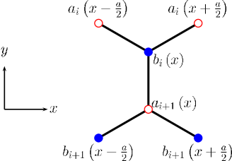
where is the current density operator of the bond from site to site , and are the corresponding amplitudes of the wave function at these sites as shown in Fig. 1, is the charge, and is the nearest-neighbor hopping parameter. Because of the translational symmetry along the -axis, the amplitudes of the wave function at the A-sublattice and B-sublattice with wave number are respectively defined as
| (2) | |||
| (3) |
The Schrdinger equations in the tight-binding model with nearest-neighbor hopping are written as
| (4) | |||
| (5) |
Here, , is the energy, and is the lattice constant.[5] In the region , a solution with exists, which is the edge state.[2] In this region, the wave amplitudes at the A- and B-sublattice are approximately written as
| (6) | |||
| (7) |
In these equations defines the width of the strip. The wave function becomes exact in the limit of either or .
In this paper, we derive a relation for the local current density in the -direction. The local current density flowing through the bond between and is written as
| (8) |
Using eqs.(4), (5), and (8), we obtain the relation between and as
| (9) |
At , namely, at the upper zigzag edge,
| (10) |
The -dependence of the local current density is calculated from the initial condition [eq.(10)] and the recurrence equation [eq.(9)]. In the edge state, where ,[6] the wave function is localized around the edges and is approximately given by eqs.(6) and (7).[7] Notice that the wave function at the A-sublattice is localized at the upper edge and that that at the B-sublattice is localized at the lower edge as shown in Fig. 2. Therefore, in the upper half of the strip, and the local current density increases as increases. At the center of the zigzag strip, is maximum since .

When or , the coupling of edges becomes small, the wave functions given by eqs.(6) and (7) become almost exact, and approaches zero. In such a situation eq.(9) implies that , namely, the current flows almost uniformly. This is also implied by eqs.(6) and (7). By substituting eqs.(6) and (7) into eq.(8), becomes independent of , and is written as
| (11) |
The energy of the edge state in such a situation is obtained from eqs.(4) and (5) to be[8]
| (12) |
The expression for the current is consistent with that obtained from the group velocity
| (13) |
at this energy.[9] When , the magnitude of the current for a state becomes small, as implied by eq.(11). However, the conductance is still , because the smallness of the current is compensated for by the large density of states.
To verify our analytical discussion, we numerically calculated the current density from eq.(1). Using Zrbo and Nikoli’s parameter , we reproduced their result[4] as shown in Fig. 3(a). With decreasing energy, the current flows almost uniformly in the -direction as shown in Fig. 3(b). These results are consistent with those derived from eq.(9).


In summary, a finite-width strip with zigzag edges has edge states with energy , and electrons are strongly localized around the edges. However, the current flows almost uniformly at the center and decreases towards the edges. This behavior is understood by the expression for the local current density in the -direction. This uniform current is realized as a result of three factors. Firstly, the wave function of the edge states decays exponentially towards the other edge. Secondly, graphene consists of an A-sublattice and B-sublattice. Thirdly, the local current density is calculated by the multiplication of amplitudes on both sublattices.[3]
In this short note we considered the current distribution of an edge state specified by wave number . The interaction between electrons is not taken into account. We remark that the possibility of magnetic ordering of the edge state has been suggested by several authors.[2, 10, 11]
Acknowledgments
We thank Yusuke Kato and Daisuke Takahashi for helpful discussions. YN acknowledges support by a Grant-in-Aid for JSPS Fellows (204840).
References
- [1] P. R. Wallace: Phys. Rev. 71 (1947) 622.
- [2] M. Fujita, K. Wakabayashi, K. Nakada, and K. Kusakabe: J. Phys. Soc. Jpn. 65 (1996) 1920.
- [3] F. Muñoz-Rojas, D. Jacob, J. Fernández-Rossier, and J. J. Palacios: Phys. Rev. B 74 (2006) 195417.
- [4] L. P. Zrbo and B. K. Nikoli: Europhys. Lett. 80 (2007) 47001.
- [5] Since and can be real, we choose them to be real hereafter.
- [6] A. Cresti, G. Grosso, and G. P. Parravicini: Phys. Rev. B 77 (2008) 115408.
- [7] K. Wakabayashi, M. Fujita, H. Ajiki, and M. Sigrist: Phys. Rev. B 59 (1999) 8271.
- [8] The expression for the energy in ref. \citenwaka2, eq.(3.12), is not correct.
- [9] For a strip of length , . Thus, the total current is , as expected.
- [10] Y.-W. Son, M. L. Cohen, and S. G. Louie: Phys. Rev. Lett. 97 (2006) 216803.
- [11] L. Pisani, J. A. Chan, B. Montanari, and N. M. Harrison: Phys. Rev. B 75 (2007) 064418.