Effects of impurities in Spin Bose-Metal phase on a two-leg triangular strip

Abstract

We study effects of nonmagnetic impurities in a Spin Bose-Metal (SBM) phase discovered in a two-leg triangular strip spin-1/2 model with ring exchanges (D. N. Sheng et al., arXiv:0902.4210). This phase is a quasi-1D descendant of a 2D spin liquid with spinon Fermi sea, and the present study aims at interpolating between the 1D and 2D cases. Different types of defects can be treated as local energy perturbations, which we find are always relevant. As a result, a nonmagnetic impurity generically cuts the system into two decoupled parts. We calculate bond energy and local spin susceptibility near the defect, both of which can be measured in experiments. The Spin Bose-Metal has dominant correlations at characteristic incommensurate wavevectors that are revealed near the defect. Thus, the bond energy shows a static texture oscillating as a function of distance from the defect and decaying as a slow power law. The local spin susceptibility also oscillates and actually increases as a function of distance from the defect, similar to the effect found in the 1D chain [S. Eggert and I. Affleck, Phys. Rev. Lett. 75, 934 (1995)]. We calculate the corresponding power law exponents for the textures as a function of one Luttinger parameter of the SBM theory.

I Introduction

There has been much interest in spin liquid phases and much progress has been made in our theoretical understanding of these (see Ref. LeeNagaosaWen, for a review). However, only recently several experimental candidates have emerged. Among these, the triangular lattice based organic compound $\kappa$-(ET)₂Cu₂(CN)₃ shows strong evidence of a gapless spin liquid. Shimizu03 ; Kurosaki05 ; SYamashita08 ; MYamashita09 One proposed theoretical state has a Fermi surface of fermionic spinons. This appears as a good variational stateringxch for an appropriate spin model with ring exchanges and also as an appealing state in a slave particle studySSLee of the Hubbard model near the Mott transition, leading to a U(1) gauge theory description.

The variational study is not sufficient to prove that a given state is realized in the system, and the 2D gauge theory does not give reliable information about the long-distance behavior. Driven by the need for a controlled theoretical access to such phases, Ref. Sheng09, considered the Heisenberg plus ring model on a two-leg triangular strip and found a ladder descendant of the 2D spin liquid in a wide regime of parameters; it also developed a Bosonization description of the quasi-1D state.

The present work is motivated by ¹³C NMR experiments Kawamoto04 ; Shimizu06 ; Kawamoto06 ; Itou08 in the organic spin liquid material that observed strong inhomogeneous line broadening at low temperatures. Theoretical Ref. Gregor08, studied effects of nonmagnetic impurities in the candidate spin liquid with spinon Fermi surface and calculated the local spin susceptibility using mean field approach. The susceptibility has an oscillating $2k_{F}$ component decaying with a $1/x$ power law envelope. A more complete gauge theory treatment is expected to modify this power law,Kim03 ; Kolezhuk06 ; Gregor08 but one cannot calculate the exponent quantitatively.

For comparison, the 1D Heisenberg chain can be loosely viewed as a 1D version of the spinon Fermi sea state,KimLee and in this case the staggered component of the local susceptibility grows away from an impurity as $x^{1/2}$ in the limit of zero temperature and zero field. This was discovered by Eggert and AffleckEggert92 ; Eggert95 and is responsible for strong inhomogeneous line broadening observed in several 1D spin-1/2 chain materials.Takigawa ; Fujiwara

In this paper we calculate effects of nonmagnetic impurities in the two-leg ladder descendant of the spin liquid using analytical approaches developed in Ref. Sheng09, , in the hope of obtaining some interpolation between the 1D chain and 2D spin liquid. We find strong enhancement of the $2k_{F}$ components of the local susceptibility compared with the mean field. The susceptibility increases away from an impurity as $\sim x^{1/2-g/4}\geq x^{1/4}$, where $g$ is one Luttinger parameter describing the phaseSheng09 and can take values $g<1$. This is a slower increase than in the 1D chain, but is still a dramatic effect. We also calculate bond textures around the defect.

II Non-magnetic impurities in the Spin Bose-Metal on the ladder

The spin system resides on the two-leg triangular ladder shown in Fig. 1, which we can also view as a zigzag chain. Throughout we assume that the model is in the described descendant phase, which we will refer to as “Spin Bose-Metal” (SBM) following Ref. Sheng09, . Examples of non-magnetic defects are shown in Fig. 1 and are discussed in detail later. Generally speaking, even though there are different types of defects, we find that they eventually (at low energies) cut the system into finite sections with essentially open boundary conditions.Kane92 ; Eggert92 ; Eggert95 We can then perform analytical calculations in a semi-infinite system studying physical properties as a function of the distance from the boundary. In the following, we focus on induced textures in two measurable quantities – the bond energy and local spin susceptibility. The physics is that an impurity perturbation has components on all wavevectors and can directly “nucleate” the dominant bond energy correlations. The impurity also allows the uniform external magnetic field to couple to the dominant spin correlations, producing textures in the local susceptibility.

Following the description in Ref. Sheng09, , there are three gapless modes with the fixed-point Lagrangian density

$${\cal L}_{\rm SBM} = \frac{1}{2\pi g}\left[\frac{1}{v}\left(\partial_{\tau}\theta_{\rho-}\right)^{2}+v\left(\partial_{x}\theta_{\rho-}\right)^{2}\right]$$

$$+ \sum_{a=1,2}\frac{1}{2\pi}\left[\frac{1}{v_{a}}\left(\partial_{\tau}\theta_{a\sigma}\right)^{2}+v_{a}\left(\partial_{x}\theta_{a\sigma}\right)^{2}\right]~{}.$$

Schematically, one route to this theorySheng09 is via a Bosonization treatment of electrons at half-filling on the ladder, where we start with two bands, $a=1,2$, and assume that the umklapp gaps out only the overall charge mode $\theta_{\rho+}$ while the other three modes $\theta_{\rho-}$, $\theta_{1\sigma}$, and $\theta_{2\sigma}$ remain gapless. Note that in this paper, we simply postulate SBM phase and do not discuss how to stabilize it. However, our intuition is that with long-ranged repulsive interaction between electrons, we can make (relatively stable) C2S2 metallic phase (with four gapless modes $\rho_{+},\rho_{-},1\sigma,2\sigma$) go to the SBM phase, which is C1S2 Mott insulator with the overall charge mode $\rho+$ gapped by appropriate umklapp process. In addition, $g_{1\sigma}$ and $g_{2\sigma}$ are equal to 1 because of SU(2) spin invariance.

Ref. Sheng09, describes various observables in the SBM. For the magnetic susceptibility calculations, we will need the spin operator. The $S^{z}$ component under Bosonization is

$$S^{z}(x)\simeq\frac{\partial_{x}(\theta_{1\sigma}+\theta_{2\sigma})}{\sqrt{2}\pi}+\sum_{Q}S^{z}_{Q}(x)e^{iQx}~{}.$$ (2)

The most important wavevectors are $Q=\pm 2k_{F1}$, $\pm 2k_{F2}$, $\mp(k_{F1}+k_{F2})=\pm\pi/2$, and $\pi$. Each term can be expressed as in Ref. Sheng09, :

$$S^{z}_{2k_{Fa}} = -e^{i\theta_{\rho+}}e^{\pm i\theta_{\rho-}}\sin(\sqrt{2}\theta_{a\sigma})~{},$$ (3)

$$S^{z}_{\pi/2} = e^{-i\theta_{\rho+}}\Big{[}-i\eta_{1\uparrow}\eta_{2\uparrow}e^{-i\theta_{\sigma+}}\sin(\varphi_{\rho-}+\varphi_{\sigma-})$$

$$~{}~{}~{}~{}~{}~{}~{}~{}~{}+i\eta_{1\downarrow}\eta_{2\downarrow}e^{i\theta_{\sigma+}}\sin(\varphi_{\rho-}-\varphi_{\sigma-})\Big{]}~{},$$

$$S^{z}_{\pi} = [\alpha\sin(2\theta_{\sigma+})+\alpha^{\prime}\sin(2\theta_{\sigma-})]\sin(2\theta_{\rho+})~{}.$$ (5)

Throughout, we keep $\theta_{\rho+}$ general, but it is understood to be pinned; details about the pinning value as well as the Klein factors $\eta_{a\sigma}$ can be found in Ref. Sheng09, . In the first line, the upper or lower sign corresponds to $a=1$ or $2$. We also introduce combinations $\theta_{\sigma\pm}=(\theta_{1\sigma}\pm\theta_{2\sigma})/\sqrt{2}$ and similarly for the conjugate fields $\varphi_{\sigma\pm}$. In the last line, $\alpha$ and $\alpha^{\prime}$ are independent numerical constants.

When discussing non-magnetic defects and also in the bond energy texture calculations, we need $n$-th neighbor bond energy operator like

$$B^{(n)}(x)\equiv\vec{S}_{x}\cdot\vec{S}_{x+n}~{}.$$ (6)

The bosonized form can be obtained from Ref. Sheng09, :

$$B^{(n)}\simeq\sum_{a=1,2}B^{(n)}_{2k_{Fa}}+B^{(n)}_{4k_{F1}}+B^{(n)}_{\pi/2}~{},$$ (7)

where we keep only the most important wavevectors and

$$B_{2k_{Fa}}^{(n)}(x)\sim\cos{(\sqrt{2}\theta_{a\sigma})}$$ (8)

$$\hskip 42.67912pt\times\cos{(2k_{Fa}x+\gamma^{(n)}_{2k_{Fa}}+\frac{\pi}{2}+\theta_{\rho+}\pm\theta_{\rho-})}~{},$$

$$B_{4k_{F1}}^{(n)}(x)\sim\cos{(4k_{F1}x+\gamma^{(n)}_{4k_{F1}}+2\theta_{\rho+}+2\theta_{\rho-})}~{},$$ (9)

$$B_{\pi/2}^{(n)}(x)\sim$$ (10)

$$-i\eta_{1\uparrow}\eta_{2\uparrow}\cos{(\frac{\pi}{2}x+\gamma^{(n)}_{\frac{\pi}{2}}-\theta_{\rho+}-\theta_{\sigma+})}\sin{(\varphi_{\rho-}+\varphi_{\sigma-})}$$

$$-i\eta_{1\downarrow}\eta_{2\downarrow}\cos{(\frac{\pi}{2}x+\gamma^{(n)}_{\frac{\pi}{2}}-\theta_{\rho+}+\theta_{\sigma+})}\sin{(\varphi_{\rho-}-\varphi_{\sigma-})}.$$

We do not show real factors in front of all terms. Here $\gamma^{(n)}_{Q}$ are phases that depend on $Q$ and the bond type:

$$\gamma^{(n)}_{Q}=nQ/2~{},$$ (11)

valid for $Q\neq\pi$. Note also that since $4k_{F2}=-4k_{F1}\mod 2\pi$, there is only one independent term $B_{4k_{F1}}$.

II.1 Nonmagnetic defects treated as perturbations

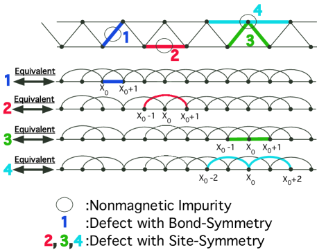
Figure 1: The top figure represents the original 2-leg triangular ladder model with ring exchanges, and the thick lines represent the defects due to the impurities. The bottom figures represent the corresponding defects in the equivalent 1D model.Sheng09 1) represents the defect symmetric with respect to a bond center, while 2), 3), and 4) represent defects symmetric about a site of the 1D chain. In general, different impurities will lead to different fixed points. Impurity 1) will likely lead to a fixed point with decoupled semi-infinite systems and a non-magnetic cluster containing an even number of sites, while impurities 2), 3), and 4) will likely lead to a fixed point with decoupled semi-infinite systems and an effective spin formed by a cluster with an odd number of sites.

When a nonmagnetic defect is introduced at $x_{0}$, we can treat it as a local perturbation in the Hamiltonian.Eggert92 ; Kane92 Figure 1 shows some possible defects; the corresponding perturbations are

$$\delta H^{(1)} \sim \vec{S}(x_{0})\cdot\vec{S}(x_{0}+1)\sim B^{(1)}(x_{0})~{},$$ (12)

$$\delta H^{(2)} \sim \vec{S}(x_{0}-1)\cdot\vec{S}(x_{0}+1)\sim B^{(2)}(x_{0}-1)~{},$$ (13)

$$\delta H^{(3)} \sim \vec{S}(x_{0})\cdot\left[\vec{S}(x_{0}-1)+\vec{S}(x_{0}+1)\right]$$ (14)

$$\sim B^{(1)}(x_{0}-1)+B^{(1)}(x_{0})~{},$$ (15)

$$\delta H^{(4)} \sim \vec{S}(x_{0})\cdot\left[\vec{S}(x_{0}-2)+\vec{S}(x_{0}+2)\right]$$ (16)

$$\sim B^{(2)}(x_{0}-2)+B^{(2)}(x_{0})~{}.$$ (17)

Here $B^{(1)}$ and $B^{(2)}$ are given by Eq. (7). We can characterize the defects by symmetry. In the 1D chain picture, $\delta H^{(1)}$ represents defects symmetric under inversion in a bond center, while $\delta H^{(2,3,4)}$ are defects symmetric under inversion in a site. One can readily check that $\delta H^{(2,3,4)}$ give equivalent expressions up to constant factors and, importantly, contain all $Q$ modes in general. We see that although the defects can be characterized as two distinct symmetry types $\delta H^{(1)}$ and $\delta H^{(2)}$, the perturbations to the Hamiltonian have the same dynamical field content and differ only by constant phases. This is unlike the Bethe phase of the 1D Heisenberg chain where a bond-symmetric perturbation contains a relevant contribution from a $Q=\pi$ bond operator while a site-symmetric perturbation does not. Eggert92

The scaling dimensions of the different contributions are

$$\Delta[B_{2k_{Fa}}] = \frac{1}{2}+\frac{g}{4}~{},$$ (18)

$$\Delta[B_{4k_{F1}}] = g~{},$$ (19)

$$\Delta[B_{\pi/2}] = \frac{1}{2}+\frac{1}{4g}~{}.$$ (20)

In the Spin Bose-Metal phase we have $g\leq 1$, so the $2k_{Fa}$ and $4k_{F1}$ terms are always relevant 0+1D perturbations, while the $\pi/2$ term is relevant if $g>1/2$. The relevant perturbations grow and one scenario is that they eventually pin the fields at the origin. Physically this leads to breaking the chain into two decoupled semi-infinite systems, which we can then study separately. The pinning conditions on the fields at the defect can be guessed by considering the most relevant perturbation and minimizing the corresponding energy. We expect the $B_{2k_{Fa}}$ and $B_{4k_{F1}}$ terms to be the dominant, which would

$${\rm Pin}~{}\theta_{1\sigma}(x_{0}),~{}\theta_{2\sigma}(x_{0}),~{}\theta_{\rho-}(x_{0})~{}.$$ (21)

This is the case that we focus on. In Appendix B we will consider pinning conditions preferred by the $B_{\pi/2}$ term, which may be of interest in the borderline case $g=1$.

A comment is in order. On physical grounds, the symmetry of the defect perturbation is important. For the case with no site inversion symmetry like the impurity 1) in Fig. 1, we can envision a possible outcome of the RG growth of the perturbation by considering a situation where the defect bond is strong. The two spins will form a singlet, and if we integrate it out, we get two semi-infinite chains weakly coupled to each other, which under further RG will eventually flow to decoupled semi-infinite systems with pinned values of the fields at the boundary. We can envision more general situations where an even number of spins will form a strongly coupled cluster with a singlet ground state, and upon integrating this out we again have two weakly coupled semi-infinite systems. Below, we will consider a fixed point of a semi-infinite system and give physical calculations of the bond textures and the oscillating susceptibility near the boundary (impurity). Turning to the case with impurities with site inversion symmetry like 2), 3), 4) in Fig. 1, such reasoning would give us a half-integer spin (formed by some effective strongly coupled cluster with an odd number of sites) weakly coupled to two semi-infinite systems. This would need to be analyzed further, which we briefly discuss in Sec. II.3.

II.2 Physical calculations of oscillating susceptibility and bond textures in the fixed-point theory of semi-infinite chains

From now on, we set the location of the defect to be the origin. We work with a semi-infinite system with specified boundary conditions at the origin and calculate the bond energy texture

$$\langle B(x)\rangle=\sum_{a=1,2}\langle B_{2k_{Fa}}(x)\rangle+\langle B_{4k_{F1}}(x)\rangle+\langle B_{\frac{\pi}{2}}(x)\rangle~{}.$$ (22)

We also calculate the local spin susceptibility, which can be measured in Knight shift experiments. We will see that there are contributions that oscillate as a function of distance from the boundary: $\chi(x)=\chi^{uni}(x)+\chi^{osc}(x)$; in fact, $\chi^{osc}(x)$ dominates over $\chi^{uni}(x)$ and can produce strong inhomogeneous broadening of the NMR lineshapes. The local spin susceptibility $\chi(i)$ at a lattice site $i$ measured in a small uniform magnetic field $h$ is

$$\chi(i)\equiv\frac{\partial\langle S_{i}^{z}\rangle}{\partial h}\Big{|}_{h=0}=\beta\langle S_{i}^{z}S_{\rm tot}^{z}\rangle~{},$$ (23)

where $S_{\rm tot}^{z}\equiv\sum_{j}S_{j}^{z}$ is the total spin and $\beta$ is the inverse temperature. Rewriting the spin operators in terms of bosonic fields introduced above,

$$\chi^{osc}(x)=\beta\left\langle S^{z}_{osc}(x)\int_{0}^{\infty}dyS^{z}_{uni}(y)\right\rangle~{},$$ (24)

where $S^{z}_{osc}=\sum_{Q}e^{iQx}S^{z}_{Q}$ and we are interested in $Q=2k_{F1}$, $2k_{F2}$, $\pi/2$, and $\pi$; while $S^{z}_{uni}(y)=\sum_{a=1,2}\frac{\partial_{y}\theta_{a\sigma}(y)}{\sqrt{2}\pi}$. Hence we define

$$\chi^{osc}_{Q}\equiv\beta\langle e^{iQx}S^{z}_{Q}(x)\int_{0}^{\infty}dyS^{z}_{uni}(y)+{\rm c.c.}\rangle~{}.$$ (25)

We consider the pinning Eq. (21) driven by the relevant local terms $B_{2k_{Fa}},B_{4k_{F1}}$; in order to minimize these energies, the natural pinning values of $\theta_{1\sigma}(0)$ and $\theta_{2\sigma}(0)$ are

$$\cos[\sqrt{2}\theta_{a\sigma}(0)]=\pm 1\Rightarrow\sqrt{2}\theta_{a\sigma}(0)={\rm integer}\times\pi~{}.$$ (26)

The pinning value of the field $\theta_{\rho-}$ depends on the details such as the amplitudes and phases $\gamma$ in Eqs. (8)-(10). As discussed in Appendix A, the pinning of a $\theta$ at the origin implies stronger fluctuation of the dual field $\varphi$ and consequently $\langle e^{i\varphi(x)}\rangle=0$.

Bond energy texture is given by Eq. (22). The $\langle B_{\pi/2}(x)\rangle$ term vanishes and the other contributions can be easily derived by applying the formulas in Appendix A:

$$\langle B_{2k_{Fa}}(x)\rangle \simeq \frac{A_{2k_{Fa}}\cos(2k_{Fa}x+\delta_{2k_{Fa}})}{\left[\frac{v_{a}\beta}{\pi}\sinh(\frac{2\pi x}{v_{a}\beta})\right]^{\frac{1}{2}}\left[\frac{v\beta}{\pi}\sinh(\frac{2\pi x}{v\beta})\right]^{\frac{g}{4}}}~{},$$ (27)

$$\langle B_{4k_{F1}}(x)\rangle \simeq \frac{A_{4k_{F1}}\cos(4k_{F1}x+\delta_{4k_{F1}})}{\left[\frac{v\beta}{\pi}\sinh(\frac{2\pi x}{v\beta})\right]^{g}}~{},$$ (28)

where $a=1,2$; $A_{Q}$ are some amplitudes; and $\delta_{Q}$ are phases that depend on the pinned $\theta$ values at the origin and are ultimately determined by the details of the defect. At low temperature $T\to 0$, we have the following behavior as a function of the distance $x$ from the open boundary (defect):

$$\langle B_{2k_{Fa}}(x)\rangle \sim \frac{\cos(2k_{Fa}x+\delta_{2k_{Fa}})}{x^{\frac{1}{2}+\frac{g}{4}}}~{},$$ (29)

$$\langle B_{4k_{F1}}(x)\rangle \sim \frac{\cos(4k_{F1}x+\delta_{4k_{F1}})}{x^{g}}~{}.$$ (30)

Thus, at low temperature the bond energy texture around the impurity reveals the correlations present in the system, and the physics can be viewed as a “nucleation” of the dominant “bond orders” near the defect. If we can tune the Luttinger parameter $g$, we see that there are two regimes: for $2/3<g<1$ the $2k_{Fa}$ terms dominate, while for $g<2/3$ the $4k_{F1}$ dominates.

Turning to the oscillating susceptibility, the $\chi^{osc}_{\pi/2}$ term vanishes and only the $\chi^{osc}_{2k_{Fa}}$ and $\chi^{osc}_{\pi}$ contribute to the final result. Applying the formulas from Appendix A gives

$$\chi^{osc}_{2k_{Fa}} \simeq \frac{C_{2k_{Fa}}\cdot x\cdot\cos(2k_{Fa}x+\delta_{2k_{Fa}}^{\prime})}{\left[\frac{v_{a}\beta}{\pi}\sinh\left(\frac{2\pi x}{v_{a}\beta}\right)\right]^{\frac{1}{2}}\left[\frac{v\beta}{\pi}\sinh\left(\frac{2\pi x}{v\beta}\right)\right]^{\frac{g}{4}}}~{},$$ (31)

$$\chi^{osc}_{\pi} \simeq \frac{C_{\pi}\cdot x\cdot(-1)^{x}}{\left[\frac{v_{1}\beta}{\pi}\sinh\left(\frac{2\pi x}{v_{1}\beta}\right)\right]^{\frac{1}{2}}\left[\frac{v_{2}\beta}{\pi}\sinh\left(\frac{2\pi x}{v_{2}\beta}\right)\right]^{\frac{1}{2}}}~{},$$ (32)

where $a=1,2$; $C_{Q}$ are some constant amplitudes; and $\delta_{Q}^{\prime}$ some phases absorbing all pinned field values and eventually determined by the details of the defect. At low temperatures $T\to 0$, the oscillating susceptibilities at $2k_{Fa}$ and $\pi$ become

$$\chi^{osc}_{2k_{Fa}}(x) \sim x^{\frac{1}{2}-\frac{g}{4}}\cos{(2k_{Fa}x+\delta_{2k_{Fa}}^{\prime})}~{},$$ (33)

$$\chi^{osc}_{\pi}(x) \sim x^{0}(-1)^{x}~{}.$$ (34)

The envelope function in the first line satisfies $x^{\frac{1}{2}-\frac{g}{4}}\geq x^{\frac{1}{4}}$, which comes from the condition $g<1$. Therefore, at low temperatures the oscillating susceptibility at $2k_{Fa}$ actually increases with the distance from the open end. On the other hand, the oscillating susceptibility at $\pi$ reaches a constant amplitude.

To conclude the discussion of the semi-infinite system with the boundary conditions Eq. (21), we note that this fixed point is stable [e.g., the scaling dimension of $B_{\pi/2}(0)$ becomes $1/2+1/(2g)>1$, so it is irrelevant]. The boundary spin operator has scaling dimension 1: e.g., $S^{z}_{\rm bound.}\sim\partial_{x}(\theta_{1\sigma}+\theta_{2\sigma})$ at the boundary. Knowing the fixed-point theory of the semi-infinite chain, we can briefly discuss other situations with impurities. Eggert92 ; Rommer98 ; Rommer00 ; Eggert01 (For a recent review of impurity problems, see Ref. Affleck08, .)

II.3 Other Situations with Impurities

II.3.1 Weakly coupled semi-infinite systems

In this case, we imagine two semi-infinite chains coupled to each other at the origin. Since in each semi-infinite system the scaling dimension of the boundary spin operator is $1$, the spin-spin coupling between the two systems is irrelevant and they will decouple at low energies. This is the reason why a non-magnetic impurity like 1) in Fig. 1 breaks the system into two halves at low energies and the physical calculations in Sec. II.2 apply generically.

II.3.2 Spin-$\frac{1}{2}$ impurity coupled to a semi-infinite system

In this case, the spin-1/2 impurity is coupled to the boundary spin operator which contains contributions from both “$1\sigma$” and “$2\sigma$” channels, $\delta H=\lambda\vec{S}_{\rm imp}\cdot(\vec{S}_{\rm bound.,1}+\vec{S}_{\rm bound.,2})\to\lambda_{1}\vec{S}_{\rm imp}\cdot\vec{S}_{\rm bound.,1}+\lambda_{2}\vec{S}_{\rm imp}\cdot\vec{S}_{\rm bound.,2}$. (The “$\rho-$” sector does not enter in the important terms.) The couplings $\lambda_{1}$ and $\lambda_{2}$ are both marginal. If they are marginally irrelevant, the impurity spin will decouple. If one of the couplings is marginally relevant while the other is marginally irrelevant, the relevant coupling will grow and the impurity spin will be absorbed into the corresponding channel. Finally, if both of the couplings are relevant, since the two channels are not equivalent, one coupling will grow faster; a likely scenario is that the impurity spin will be absorbed into the dominating channel and eventually the two channels will decouple.

II.3.3 Two semi-infinite systems coupled symmetrically to a spin-$\frac{1}{2}$ impurity

Now let us take two semi-infinite chains and couple them together through a spin-1/2 impurity symmetrically. This case is also relevant for the site-symmetric non-magnetic impurities like impurity 2), 3), and 4) in Fig. 1: The reason is that because of the site inversion symmetry, the non-magnetic impurity affects an even number of bonds which couple an odd number of spins; then we can imagine a strongly-coupled cluster with the odd number of spins, which will effectively behave as a half-integer spin weakly coupled to the left and right semi-infinite systems.

The situation is more complex than in the previous subsection because we now have symmetry between the two semi-infinite systems, reminiscent of the 2-channel Kondo problem. We can imagine the following possibilities. When all couplings are marginally irrelevant, the impurity spin and the two semi-infinite systems will decouple at low energies (and the physical calculations of textures in Sec. II.2 are valid in this case). Suppose now we have marginally relevant couplings and the dominant growth is for the channels $1\sigma$ in the two semi-infinite systems. One is tempted to speculate about the possibility of “healing” the channels $1\sigma$ across the impurity, while the channels $2\sigma$ remain open. However, it is likely that this is not a stable fixed point in the presence of the allowed terms in the Hamiltonian coming from the microscopic ladder system. While the eventual outcome is not clear and depends on details, on physical grounds we again expect arriving at some stage at a fixed point with some odd number of spins forming a half-integer spin that is decoupled from two semi-infinite systems.

III Conclusions

To summarize, following the theoretical descriptionSheng09 of the Spin Bose-Metal phase in the triangular strip spin-1/2 model with ring exchanges, we discussed the effects due to different types of impurities. The defects can have additional bond or site symmetry in the 1D zigzag chain language. We first treated the defects as local perturbations in the Hamiltonian and saw that all types produce relevant perturbations, eventually breaking the system into two halves and a separate decoupled cluster of spins. In the bond-symmetric case (or more general cases with no symmetries) the decoupled cluster is likely to be non-magnetic, while in the site-symmetric case it has half-integer spin, and the details of such fixed points depend on the microscopic details.Eggert92 ; Rommer00 ; Eggert01 This analysis also motivated appropriate boundary conditions for pinning the fields in the fixed point theory for the semi-infinite systems.

For such a semi-infinite chain, we calculated the bond energy texture near the boundary and found power law decays Eqs. (27, 28) of the oscillating components at wavevectors $2k_{Fa}$, $4k_{F1}$. The dominant power law switches from the $2k_{Fa}$ to the $4k_{F1}$ when the Luttinger parameter $g$ drops below $2/3$. We suggest that characterizing such bond textures in numerical studies, e.g. DMRG,Sheng09 could be useful for determining the Luttinger parameter $g$ of the SBM theory.

We also calculated the oscillating susceptibilities at $2k_{Fa}$ and $\pi$, Eqs. (31, 32), which behave differently at low temperatures. The susceptibilities at $2k_{Fa}$ actually increase with the distance from the boundary in the limit of zero temperature (and zero field), while the susceptibility at $\pi$ becomes distance-independent. Transfer-Matrix density-matrix Renormalization Group (TMRG) Rommer98 ; Rommer00 ; TMRG96 technique can measure local susceptibility at finite temperature and can be useful for exploring the susceptibility near defects in numerical studies. The rate of increase at $2k_{Fa}$ is slower than in the 1D chain,Eggert95 but would still produce strong NMR line broadening at low temperatures. Of course, this is the result for the long-distance behavior along the 1D direction. If we are thinking about the 2D spin liquid, we would likely expect a power-law decay away from an impurity.Kim03 ; Kolezhuk06 ; Gregor08 Nevertheless, the persistence of the oscillating susceptibilities on the quas-1D ladders suggests that in the 2D case the decay may be slow and also produce significant inhomogeneous line broadening. Finally, in this paper, we focused on non-magnetic impurities and the simplest “fixed-point” model with open boundary. We have not touched interesting and experimentally relevant crossovers present for a magnetic impurity weakly coupled to the system.Rommer98 ; Rommer00 Here again theoretical and numerical studies similar to Ref. Rommer98, ; Rommer00, could be very helpful, for example, in estimating the size of the Kondo screening cloud, which is an additional and potentially large effect near the magnetic impurity.

Appendix A One mode theory on a semi-infinite chain

For the simplest case,Eggert92 ; Eggert95 ; Rommer00 ; Bortz05 consider a one mode theory on a semi-infinite chain with pinned value at the origin, $\theta(0,\tau)=pinned=\theta_{0}$. The action is

$$S=\int_{0}^{\infty}dx\int_{0}^{\beta}d\tau\frac{1}{2\pi g}\left[v(\partial_{x}\theta)^{2}+\frac{1}{v}(\partial_{\tau}\theta)^{2}\right]~{}.$$ (35)

The correlation functions needed in this paper are

$$\left\langle e^{iu\theta(x,\tau)}\right\rangle\simeq\frac{Ae^{iu\theta_{0}}}{[\frac{v\beta}{\pi}\sinh{(\frac{2\pi x}{v\beta})}]^{\frac{u^{2}g}{4}}}~{},$$ (36)

$$\left\langle e^{iu\theta(x,\tau)}\int_{0}^{\infty}dy\frac{\partial_{y}\theta(y,\tau^{\prime})}{\pi}\right\rangle=\frac{iugx}{\beta v}\times\left\langle e^{iu\theta(x,\tau)}\right\rangle$$ (37)

$$\hskip 71.13188pt\simeq\frac{iugx}{\beta v}\frac{Ae^{iu\theta_{0}}}{[\frac{v\beta}{\pi}\sinh{(\frac{2\pi x}{v\beta})}]^{\frac{u^{2}g}{4}}}~{},$$ (38)

$$\left\langle e^{iu\varphi(x,\tau)}\right\rangle=0~{}.$$ (39)

Here $u$ is a parameter depending on which quantity is being measured and $A$ is some real constant. The $\langle e^{iu\theta}\rangle$ is non-zero because of the pinning at $x=0$ and decays as a power-law away from the origin at $T=0$. On the other hand, the conjugate field $\varphi$ fluctuates more strongly than in the bulk and $\langle e^{iu\varphi}\rangle=0$ everywhere.

We can similarly consider a one mode theory with the dual field pinned at the origin, $\varphi(0,\tau)=pinned=\varphi_{0}$. It is convenient to work with the action

$$S=\int_{0}^{\infty}dx\int_{0}^{\beta}d\tau\frac{g}{2\pi}\left[v(\partial_{x}\varphi)^{2}+\frac{1}{v}(\partial_{\tau}\varphi)^{2}\right]~{}.$$ (40)

The correlation function needed is

$$\left\langle e^{iu\varphi(x,\tau)}\right\rangle\simeq\frac{\tilde{A}e^{iu\varphi_{0}}}{[\frac{v\beta}{\pi}\sinh{(\frac{2\pi x}{v\beta})}]^{\frac{u^{2}}{4g}}}~{},$$ (41)

where $\tilde{A}$ is some constant.

Appendix B Calculations in a fixed point theory of a semi-infinite system with pinned $\theta_{\sigma+}(0)$, $\varphi_{\sigma-}(0)$, and $\varphi_{\rho-}(0)$

Here we consider the theory Eq. (II) on a semi-infinite chain with boundary conditions

$${\rm Pin}~{}\theta_{\sigma+}(0),~{}\varphi_{\sigma-}(0),~{}\varphi_{\rho-}(0)~{}.$$ (42)

This can arise if we minimize the $B_{\pi/2}(0)$ perturbation instead of the $B_{2k_{Fa}}(0)$ and $B_{4k_{F1}}(0)$, see Eqs. (8-10). Coming from the microscopic ladder spin system in the SBM phase with $g<1$, this fixed point is unstable to the allowed $B_{2k_{Fa}}(0)$ terms. Nevertheless, it can be of interest in the special case with $g=1$, which is realized, e.g., by the Gutzwiller wavefunctions or at phase transitions out of the SBM.Sheng09 The calculations of the physical textures are simple and we summarize these below.

Because of the pinning Eq. (42), the dual fields $\varphi_{\sigma+}$, $\theta_{\sigma-}$, and $\theta_{\rho-}$ fluctuate more strongly. The only non-vanishing term in the bond energy texture is

$$\langle B(x)\rangle=\langle B_{\pi/2}(x)\rangle~{}.$$ (43)

If $v_{1}=v_{2}$, then “$\sigma+$” and “$\sigma-$” variables decouple and we can apply the formulas in Appendix A. In the general case $v_{1}\neq v_{2}$, the calculations are more demanding but the result is simple:

$$\langle B_{\pi/2}(x)\rangle\simeq\frac{A_{\pi/2}\cos{(\frac{\pi}{2}x+\delta_{\pi/2})}}{\left[\frac{v_{r}\beta}{\pi}\sinh{(\frac{2\pi x}{v_{r}\beta})}\right]^{\frac{1}{2}}\left[\frac{v\beta}{\pi}\sinh{(\frac{2\pi x}{v\beta})}\right]^{\frac{1}{4g}}}~{},$$ (44)

where $\frac{1}{v_{r}}=\frac{1}{2}\left(\frac{1}{v_{1}}+\frac{1}{v_{2}}\right)$, $A_{\pi/2}$ is some amplitude and $\delta_{\pi/2}$ is a constant phase. The pinned values at the origin as well as the Klein numbers enter in the same way as they enter the assumed minimization of $B_{\pi/2}(0)$, Eq. (10), so the final result depends only on the physical details of this term at the origin. In the limit $T\to 0$,

$$\langle B_{\pi/2}(x)\rangle\sim\frac{\cos{(\frac{\pi}{2}x+\delta_{\pi/2})}}{x^{\frac{1}{2}+\frac{1}{4g}}}~{}.$$ (45)

As for the oscillating susceptibility, similarly to the bond energy texture, only the $Q=\pi/2$ term contributes to the final result. Again, for $v_{1}=v_{2}$ we can apply the formulas in Appendix A, while in the general case we get

$$\chi^{osc}_{\pi/2}\simeq\frac{C\cdot x\cdot\cos(\frac{\pi}{2}x+\delta_{\pi/2}^{\prime})}{\left[\frac{v_{r}\beta}{\pi}\sinh(\frac{2\pi x}{v_{r}\beta})\right]^{\frac{1}{2}}\left[\frac{v\beta}{\pi}\sinh(\frac{2\pi x}{v\beta})\right]^{\frac{1}{4g}}}~{},$$ (46)

where $C_{\pi/2}$ is some amplitude and $\delta_{\pi/2}^{\prime}$ is a constant phase absorbing all pinned values and eventually determined by the details of the defining energy $B_{\pi/2}(0)$. In the low temperature limit $T\to 0$,

$$\chi^{osc}_{\pi/2}\sim x^{\frac{1}{2}-\frac{1}{4g}}\cos(\frac{\pi}{2}x+\delta_{\pi/2}^{\prime})~{}.$$ (47)

References

- (1) P. A. Lee, N. Nagaosa, and X.-G. Wen, Rev. Mod. Phys. 78, 17 (2006).
- (2) Y. Shimizu, K. Miyagawa, K. Kanoda, M. Maesato, and G. Saito, Phys. Rev. Lett. 91, 107001 (2003).
- (3) Y.Kurosaki, Y. Shimizu, K. Miyagawa, K. Kanoda, and G. Saito, Phys. Rev. Lett. 95, 177001 (2005).
- (4) S. Yamashita, Y. Nakazawa, M. Oguni, Y. Oshima, H. Nojiri, Y. Shimizu, K. Miyagawa, and K. Kanoda, Nature Physics 4, 459 (2008).
- (5) M. Yamashita, N. Nakata, Y. Kasahara, T. Sasaki, N. Yoneyama, N. Kobayashi, S. Fujimoto, T. Shibauchi, and Y. Matsuda, Nature Physics 5, 44 (2009).
- (6) O. I. Motrunich, Phys. Rev. B 72, 045105 (2005).
- (7) S.-S. Lee and P. A. Lee, Phys. Rev. Lett. 95, 036403 (2005).
- (8) D. N. Sheng, O. I. Motrunich, and M. P. A. Fisher, arXiv:0902.4210
- (9) A. Kawamoto, Y. Honma, and K. I. Kumagai, Phys. Rev. B 70, 060510(R) (2004).
- (10) Y. Shimizu, K. Miyagawa, K. Kanoda, M. Maesato, and G. Saito, Phy. Rev. B 73, 140407(R) (2006); AIP Conf. Proc. 850, 1087 (2006).
- (11) A. Kawamoto, Y. Honma, K. I. Kumagai, N. Matsunaga, and K. Nomura, Phy. Rev. B 74, 212508 (2006).
- (12) T. Itou, A. Oyamada, S. Maegawa, M. Tamura, and R. Kato, Phys. Rev. B 77, 104413 (2008).
- (13) K. Gregor and O. I. Motrunich, Phys. Rev. B 79, 024421 (2009).
- (14) Y. B. Kim and A. J. Millis, Phys. Rev. B 67, 085102 (2003)
- (15) A. Kolezhuk, S. Sachdev, R. R. Biswas, and P. Chen, Phys. Rev. B 74, 165114 (2006).
- (16) D. H. Kim and P. A. Lee, Ann. Phys. (N.Y.) 272, 130 (1999).
- (17) S. Eggert and I. Affleck, Phy. Rev. B 46, 10866 (1992).
- (18) S. Eggert and I. Affleck, Phys. Rev. Lett. 75, 934 (1995).
- (19) M. Takigawa, N. Motoyama, H. Eisaki, and S. Uchida, Phys. Rev. B 55, 14129 (1997).
- (20) N. Fujiwara, H. Yasuoka, Y. Fujishiro, M. Azuma, and M. Takano, Phys. Rev. Lett. 80, 604 (1998)
- (21) C. L. Kane and M. P. A. Fisher, Phys. Rev. Lett. 68, 1220 (1992); Phys. Rev. B 46, 15233 (1992).
- (22) S. Eggert and S. Rommer, Phys. Rev. Lett. 81, 1690 (1998); Physica B 261, 200 (1999).
- (23) S. Rommer and S. Egger, Phys. Rev. B 62,4370 (2000).
- (24) S. Eggert, D. P. Gustafsson, and S. Rommer, Phys. Rev. Lett. 86, 516 (2001).
- (25) Ian Affleck, arXiv:0809.3474.
- (26) M. Bortz and J. Sirker, J. Phys. A 38 5957 (2005).
- (27) R. J. Bursill, T. Xiang, and G.A. Gehring, J. Phys. C 8, L583 (1996); X.Q. Wang and T. Xiang, Phys. Rev. B 56, 5061 (1997); N. Shibata, J. Phys. Soc. Jpn. 66, 2221 (1997).