Predictions of highest Transition-temperature for electron-phonon superconductors

Abstract

Using the Eliashberg strong coupling theory with vertex correction, we calculate maps of transition temperatures ( T_c ) of electron-phonon superconductors in full parameter space. The maximums of transition temperatures for superconductors are predicted based on the maps and the criterion of instability of superconductivity. The strong vertex correction and high transition temperature are tightly correlated in superconductors. We predict that the maximum of T_c of new iron-based superconductors will be close to 90(K).

1 Introductions

The researches to find home-temperature superconductors are still highlight in the field of material science [1]. The theoretical predictions of T_c are the main efforts of theoretical scientists working in this field. The BCS theory[2] and Eliashberg strong coupling theory [3, 4, 5, 6, 7] are well known acceptable theories to explain the superconductivity of electron-phonon superconductors. There exists the well known upper limit of T_c defined by the McMillan T_c formula [7]. The lattice instability (softening phonon) and the total strength of electron-phonon coupling also set the bounds of T_c of electron-phonon superconductors [8]. The dielectric properties have been expected to have significant influence on the possible maximum of T_c for a variety of superconductors, but the problem is still not answered because the complex relation between effective electron-electron interaction and dielectric function [9]. The magnetic fluctuation and the vertex correction (non-adiabatic effects)  [10] can suppress the T_c and lead to the instability of superconductivity of electron-phonon superconductors. .

The new novel Iron-based high-temperature superconductor [11, 12, 13, 14, 15] has been discovered and the new record of transition temperature T_c has reached about 57.4 (K) by doping rare earth elements into CaFeAsF [15]. Especially the significant normal isotope effects of iron with $\alpha\sim 0.4$  for Ba_1-xK_xFe₂As₂ indicates that electron-phonon interaction plays an essential role to explain their superconductivity [16]. The Eliashberg theory suitable for both weak-coupling and strong-coupling should be studied in more detailed. It is very desirable to study the effects of vertex correction beyond Migdal theorem [10], especially for superconductors have components of light atoms. The Eliashberg theory has been successfully used to calculate T_c of many types of superconductors [17, 18, 19]. However, only special regions in parameter space of $\lambda-\Omega_{P}-\mu^{*}$ have been explored, where $\lambda$ is the parameter of electron-phonon interaction, $\Omega_{P}$ the frequency of phonon and $\mu^{*}$ the Coulomb pseudo-potential. In this paper, we present the information ( T_c map ) in full parameter space $\lambda-\Omega_{P}-\mu^{*}$. The T_c maps obtained in this paper are very helpful to analyze the relation between T_c and these superconducting parameters and guide to find the superconductors with higher T_c.

2 Theory

In the paper, we generalize the equation of energy gap in reference [10] by including the Coulomb interaction. The standard energy-gap equation with the form of imaginary Matsubara’s formulation [5] and the equation after having considered vertex corrections are used in our calculations. For isotropic electron-phonon interaction,

$$H_{ep}=J\sum_{\alpha,pq}c^{+}_{\alpha,p}c_{\alpha,p+q}(a^{+}_{\alpha,-q}+a_{\alpha,q}),$$ (1)

the calculations of vertex corrections are greatly simplified. The electron-phonon interactions are included in the vertex corrections only by the functions of electron-phonon interaction $\lambda(n)$ defined below. The self-energy and Green’s function of electron in the Nambu scheme are expressed as

$$\hat{\Sigma}(k,i\omega_{n}) = (1-Z(k,i\omega_{n}))i\omega_{n}\hat{\tau}_{0}-\phi(k,i\omega_{n})\hat{\tau}_{1}+\chi(k,i\omega_{n})\hat{\tau}_{3},$$

$$\hat{G}(k,i\omega_{n}) = \frac{i\omega_{n}Z(k,i\omega_{n})\hat{\tau}_{0}-\phi(k,i\omega_{n})\hat{\tau}_{1}+\varepsilon_{k}(i\omega_{n})\hat{\tau}_{3}}{(i\omega_{n})^{2}Z^{2}(k,i\omega_{n})-\varepsilon^{2}_{k}(i\omega_{n})-\phi^{2}(k,i\omega_{n})},$$ (2)

where $\phi(k,i\omega_{n})$ is the function of energy gap, $Z(k,i\omega_{n})$ the renormalization function, and $\varepsilon_{k}(i\omega_{n})=\varepsilon^{0}_{k}(i\omega_{n})+\chi(k,i\omega_{n})$. In above equations $\hat{\tau}_{1}$ and $\hat{\tau}_{3}$ are two Pauli matrixes and $\hat{\tau}_{0}$ 2$\times$2 unity matrix.

If the density of state of phonon $F(\nu)=V/(2\pi)^{d}\int d^{d}pB(p,\nu)$ and its spectral function $B(p,\nu)$ are known, the effective electron-phonon interaction $\alpha^{2}(\nu)$ is defined by

$$\alpha^{2}(\nu)F(\nu)=\frac{V}{W}\int_{S}\frac{d^{d-1}p}{v_{F}}\int_{S^{\prime}}\frac{d^{d-1}p^{\prime}}{v_{F^{\prime}}}B(p-p^{\prime},\nu)|J^{e}_{p-p^{\prime}}|^{2},$$ (3)

where $W=(2\pi)^{d}\int_{S}d^{d-1}p/v_{F}$, $v^{F}$ Fermi velocity and $J^{e}_{p-p^{\prime}}$ the matrix element of electron-phonon interaction which is constant $J$ in this work. The first order self-energies of electrons contributed from electron-phonon interaction and electron-electron interaction are standard and written as

$$\hat{\Sigma}^{1}(i\omega_{n}) = k_{B}T\sum_{n^{\prime}}\lambda(n-n^{\prime})\int_{-E_{F}}^{E_{F}}d\varepsilon_{k^{\prime}}\hat{\tau}_{3}\hat{G}(\varepsilon_{k^{\prime}},i\omega_{n^{\prime}})\hat{\tau}_{3}$$ (4)

$$\hat{\Sigma}^{c}(i\omega_{n}) =- k_{B}T\sum_{n^{\prime}}\mu^{*}\int_{-E_{F}}^{E_{F}}d\varepsilon_{k^{\prime}}\hat{\tau}_{3}\hat{G}^{od}(\varepsilon_{k^{\prime}},i\omega_{n^{\prime}})\hat{\tau}_{3}$$

where $\hat{G^{od}}(\varepsilon_{k^{\prime}},i\omega_{n^{\prime}})$ is off-diagonal part of Green’s function matrix $\hat{G}(\varepsilon_{k^{\prime}},i\omega_{n^{\prime}})$. For convenience, the kinetic energy $\varepsilon_{k^{\prime}}$ has to shift $\varepsilon_{k^{\prime}}-E_{F}$ and a symmetric band from $-E_{F}$ to $E_{F}$ is chosen. Additionally we assume $k^{\prime}$-dependent $\hat{G}(k^{\prime},i\omega_{n^{\prime}})$ realized by $\hat{G}(\varepsilon_{k^{\prime}},i\omega_{n^{\prime}})$. The electron-phonon interaction is included in $\lambda(n)=2\int_{0}^{\infty}d\nu\alpha^{2}F(\nu)\nu/(\nu^{2}+\omega_{n}^{2})$. The Coulomb pseudo-potential is defined as $\mu^{*}=\mu_{0}/(1+\mu_{0}\ln(E_{F}/\omega_{0}))$, where $\mu_{0}=N(E_{F})U$, $N(E_{F})$ the density of state at Fermi energy E_F, U the Coulomb interaction between electrons and $\omega_{0}$ characteristic energy of typical phonon correlated to superconductivity.

The lowest order vertex correction comes from the second order self-energy that is written as

$$\hat{\Sigma}^{2}(k,i\omega_{n}) = (k_{B}T)^{2}|J|^{4}\Sigma_{n^{\prime}n^{\prime\prime}k^{\prime}k^{\prime\prime}}D(k-k^{\prime},i\nu_{n-n^{\prime}})D(k-k^{\prime\prime},i\nu_{n-n^{\prime\prime}})$$

$$\times \hat{\tau}_{3}\hat{G}(k^{\prime},i\omega_{n^{\prime}})\hat{\tau}_{3}\hat{G}(k^{\prime\prime\prime},i\omega_{n^{\prime\prime\prime}})\hat{\tau}_{3}\hat{G}(k^{\prime\prime},i\omega_{n^{\prime\prime}})\hat{\tau}_{3}$$

where $D(k^{*},i\nu_{n^{*}})$ is phonon Green’s function with the definitions of indexes $n^{*}$=$n-n^{\prime}$ or $n-n^{\prime\prime}$, $n^{\prime\prime\prime}=n^{\prime}+n^{\prime\prime}-n$, $k^{*}$=$k-k^{\prime}$ or $k-k^{\prime\prime}$ and $k^{\prime\prime\prime}=k^{\prime}+k^{\prime\prime}-k$. The summation $\sum_{k^{*}}$ of wave vector $k^{*}$ ($k^{*}=k^{\prime}$ or $k^{\prime\prime}$) is replaced by $V/(2\pi)^{3}\int d^{3}k^{*}=V/v_{F}(2\pi)^{3}\int d^{2}k^{*}\int d\varepsilon_{k^{*}}$. We introduce an integral $(1/2E_{F})\int^{E_{F}}_{-E_{F}}d\varepsilon_{k^{\prime\prime\prime}}$ in Eq.(2). So the second order self-energy after having averaged on Fermi surface can be simplified as

$$\hat{\Sigma}^{2}(i\omega_{n}) = \frac{(k_{B}T)^{2}}{2E_{F}}\Sigma_{n^{\prime}n^{\prime\prime}}\lambda(n-n^{\prime})\lambda(n-n^{\prime\prime})$$

$$\times \int^{E_{F}}_{-E_{F}}d\varepsilon_{k^{\prime}}\int^{E_{F}}_{-E_{F}}d\varepsilon_{k^{\prime\prime}}\int^{E_{F}}_{-E_{F}}d\varepsilon_{k^{\prime\prime\prime}}$$

$$\times \hat{\tau}_{3}\hat{G}(\varepsilon_{k^{\prime}},i\omega_{n^{\prime}})\hat{\tau}_{3}\hat{G}(\varepsilon_{k^{\prime\prime\prime}},i\omega_{n^{\prime\prime\prime}})\hat{\tau}_{3}\hat{G}(\varepsilon_{k^{\prime\prime}},i\omega_{n^{\prime\prime}})\hat{\tau}_{3}$$

now $\varepsilon_{k^{\prime\prime\prime}}$ is an independent variable. Three integrals of kinetic energy can independently be done by

$$\int^{E^{*}}_{-E^{*}}d\varepsilon_{k^{*}}\hat{G}(\varepsilon_{k^{*}},i\omega_{n})=-\pi(is_{n}\tau_{0}+\frac{\Delta_{n}}{|\omega_{n}|}\tau_{1})a_{n}$$ (7)

when temperature is very close to T_c, $\phi(k,i\omega_{n})\rightarrow 0$, so we ignore the term $\phi^{2}(k,i\omega_{n})$ in the denominator of Green’s function Eq.(2). Other parameters are defined as $s_{n}=\omega_{n}/|\omega_{n}|$, $a_{n}=(2/\pi)\arctan(E^{*}/|\omega_{n}|)$ and $\Delta_{n}=\phi(i\omega_{n})/Z(i\omega_{n})$ the energy-gap parameter. In the general situation, the second-order self-energy cannot simply be written as the functions of $\lambda(n)$. In terms of above approximation, we transform the formulas of second-order self energy to a new formation which is suitable for numerical calculations. Although effects of electron-electron correlation are not treated accurately, the above approximation is still reasonable because the main contributions to superconductivity come from $\lambda(n-n^{\prime})\lambda(n-n^{\prime\prime})$ in Eq.(2) and Eq.(2).

The total self-energy we consider is $\Sigma(i\omega_{n})=\Sigma^{1}(i\omega_{n})+\Sigma^{c}(i\omega_{n})+\Sigma^{2}(i\omega_{n})$. By combining with Dyson Equation and considering that, when temperature is very close to T_c, $\Delta_{n}\rightarrow 0$, the terms proportional to $\Delta^{2}$ are ignored and the energy-gap equation is generalized to

$$\sum_{n^{\prime}=-\infty}^{+\infty}(K_{nn^{\prime}}-\rho\delta_{nn^{\prime}})\frac{\Delta_{n^{\prime}}}{|\omega_{n^{\prime}}|}=0,$$ (8)

where the kernel matrix

$$K_{nn^{\prime}} = [\lambda(n-n^{\prime})B(nn^{\prime})-\mu^{*}+C(nn^{\prime})]a_{n^{\prime}}-\delta_{nn^{\prime}}H_{n^{\prime}},$$ (9)

$$H_{n^{\prime}} = \sum_{n^{\prime\prime}=-\infty}^{+\infty}[\delta_{n^{\prime}n^{\prime\prime}}\frac{|\omega_{n^{\prime\prime}}|}{\pi k_{B}T}+\lambda(n^{\prime}-n^{\prime\prime})A(n^{\prime}n^{\prime\prime})s_{n^{\prime}}s_{n^{\prime\prime}}a_{n^{\prime\prime}}]$$

with parameters $A(nn^{\prime})=1-V_{A}(nn^{\prime})$, $B(nn^{\prime})=1-V_{B}(nn^{\prime})$ and $a_{n}=(2/\pi)\arctan(E_{F}/Z_{n}|\omega_{n}|)$. The 3-dimensional parameters of vertex correction have the form

$$V_{A}(nn^{\prime}) = (\pi^{2}k_{B}T/2E_{F})\sum_{n^{\prime\prime}}\lambda(n-n^{\prime\prime})s_{n^{\prime}+n^{\prime\prime}-n}s_{n^{\prime\prime}}a_{n^{\prime}+n^{\prime\prime}-n}a_{n^{\prime\prime}}$$ (10)

$$V_{B}(nn^{\prime}) = (\pi^{2}k_{B}T/E_{F})\sum_{n^{\prime\prime}}\lambda(n-n^{\prime\prime})s_{n^{\prime}+n^{\prime\prime}-n}s_{n^{\prime\prime}}a_{n^{\prime}+n^{\prime\prime}-n}a_{n^{\prime\prime}}$$

$$C(nn^{\prime}) = (\pi^{2}k_{B}T/2E_{F})\sum_{n^{\prime\prime}}\lambda(n-n^{\prime\prime})\lambda(n^{\prime}-n^{\prime\prime})s_{n^{\prime}-n^{\prime\prime}+n}s_{n^{\prime\prime}}a_{n^{\prime}-n^{\prime\prime}+n}a_{n^{\prime\prime}}.$$

If we ignore the vertex corrections, three parameters $V_{A}(nn^{\prime})$, $V_{B}(nn^{\prime})$ and $C(nn^{\prime})$ are all equal to zero and the kernel Eq.(9) of energy-gap equation reduces to the general form without vertex correction [5]. At the same time, the differences of the equations of energy gap in 3-dimensional and 2-dimensional space are only included in the function $\alpha^{2}F(\nu)$ if vertex corrections are ignored. The introduction of pair-breaking parameter $\rho$ creates an eigenvalue problem. The physical gap-equation is corresponding to $\rho$=0. In the calculation of $a_{n}$, we choose $Z_{n}\sim$1 the value of normal state. The T_c is defined as the temperature when the maximum of eigenvalues E^max of kernel matrix $K_{nn^{\prime}}$ crosses zero and changes its sign. We use about N=200 Matsubara’s energies to solve above equation. The method to find T_c is similar to the bisection method used to find the roots of a nonlinear equation [20]. The nonlinear equation to find T_c is E^max(T)=0. We can reach the accurate of 0.0001(K) after only 20-30 iterations in temperature interval from 0 (K) to 600 (K).

In calculations of $\alpha^{2}F(\nu)$, we assume that $\alpha^{2}(\nu)$ is approximately a constant around the peak of phonon mode and the density of state of phonon is expressed as

$$F(\nu)=\left\{\begin{tabular}[]{cc}$\frac{c}{(\nu-\Omega_{P})^{2}+(\omega_{2})^{2}}-\frac{c}{(\omega_{3})^{2}+(\omega_{2})^{2}}$,&$|\nu-\Omega_{P}|<\omega_{3}$\\ 0&others,\end{tabular}\right.$$ (13)

where $\Omega_{P}$ is the energy of phonon mode, $\omega_{2}$ the half-width of peak of phonon mode and $\omega_{3}=2\omega_{2}$. The parameter of electron-phonon interaction is defined as $\lambda=\lambda(0)=2\int_{0}^{\infty}d\nu\alpha^{2}F(\nu)/\nu$. An important relation

$$M\langle\nu^{2}\rangle\lambda=\eta=const$$ (14)

will be used, where $M$ is the effective mass for a certain phonon mode, especially the constant $\eta$ , the so-called McMillan-Hopfiled parameter, is closely related to T_c [5]. The superconductor parameter $\eta=N(E_{F})\langle J^{2}\rangle$, characterizes the chemical environment of atoms and almost keeps as a constant against the simple structural changes or isotope substitutions.

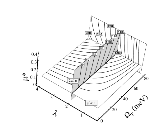
Figure 1: The 3-dimensional T_c map and three slice planes with $\lambda$=2.0, $\mu^{*}$=0.1 and $\Omega_{P}$=80 meV. The numbers within the rectangles nearby the contour lines are T_c values of the corresponding contour lines.

3 T_c Map without vertex corrections

A T_c map in full parameter-space $\lambda-\Omega_{P}-\mu^{*}$ is very helpful to understand the superconductivity with electron-phonon mechanism. At first, we choose three-dimensional 30$\times$30$\times$30 mesh-grid with 0.4$\leq\lambda\leq$4.0, 0$\leq\mu^{*}\leq$0.4 and 5.0 meV$\leq\Omega_{P}\leq$80 meV. We calculate T_c on every mesh point using Eq.(8). We plot three slice planes with $\lambda$=2.0, $\mu^{*}$=0.1 and $\Omega_{P}$=80 meV respectively shown in Fig.1. Comparing with others two parameters, the choice of $\mu^{*}$ has smaller effects on T_c. The parameter $\lambda$=2.0 is the upper limit of electron-phonon interaction [7]. When the parameter $\lambda$ is larger than 2.0, the crystal lattice will be unstable. In our calculations, the half-height width $\omega_{2}$ has the same value (4 meV ) for all points of the T_c map. If the peak of phonon mode is not too broad, the T_c map has no significant change. Conversely, the Einstein mode with $\omega_{2}\sim$0 has higher T_c.

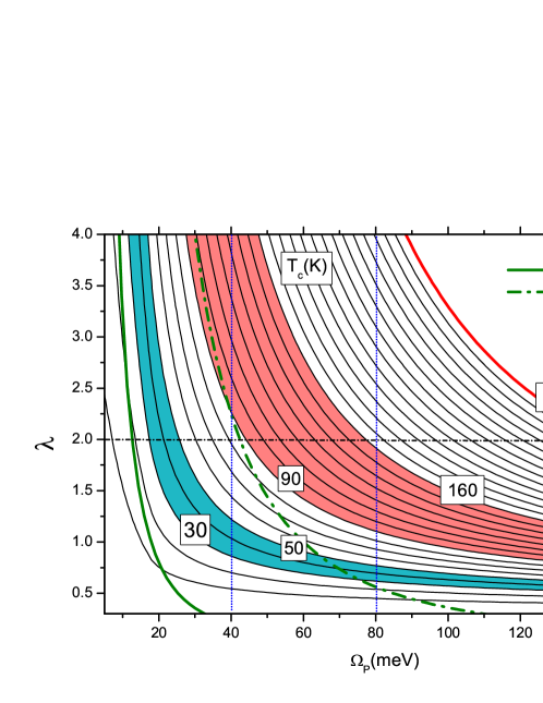
Figure 2: The T_c map in $\lambda-\Omega_{p}$ plane with $\mu^{*}$=0.10 obtained from imaginary-energy Matsubara’s method. The bold solid line and dash-dot line are the curves $\lambda\Omega^{2}_{P}$=320 (meV)² (T${}_{c}^{max}$=24 K) and 3600 (meV)² (T${}_{c}^{max}$=80 K) respectively.

In Fig.2, we plot a T_c map in two-dimensional $\lambda-\Omega_{P}$ plane in details using 50$\times$100 mesh-grid with parameters $\lambda$ from 0.4 to 4.0, $\Omega_{P}$ from 5 meV to 160 meV and the Coulomb pseudo-potential $\mu^{*}$=0.1. The two-dimensional map is the extension of the slice of the corresponding 3-dimensional map with $\mu^{*}$=0.1 shown in Fig.1. The important role of the relation $M\langle\nu^{2}\rangle\lambda$=const of Eq.(14) can be shown clearly on the T_c map. If the effective mass M of a certain phonon mode is constant, so is the parameter $\langle\nu^{2}\rangle\lambda$. We assume the half-width of peak of phonon mode $\omega_{2}\ll\Omega_{p}$, so $\langle\nu^{2}\rangle\lambda\sim\Omega^{2}_{P}\lambda$=const. The two curves of $\Omega^{2}_{P}\lambda$=320 and 3600 (meV)² are plotted in the same map. In the regime of strong coupling, $k_{B}T_{c}$ is approximately equal to $a\sqrt{\langle\nu^{2}\rangle\lambda}$ $\sim$ $a\sqrt{\Omega^{2}_{P}\lambda}$, where $a$=0.115. Thus $\langle\nu^{2}\rangle\lambda$=const is equivalent to T_c=const. In fact, $\langle\nu^{2}\rangle\lambda$=const was used to define the possible maximum of T_c [7]. The T_c increases with $\lambda$ and saturates at $\lambda=2$ by using the McMillan formula. Similar to McMillan’s idea, our results in the Fig.2 just show that the two curves coincide approximately with the contour lines of T_c in strong-coupling regime. The approximate saturations happen when $\lambda$ is very close to 2.

The term $\langle\nu^{2}\rangle\lambda$ characterizes the possible maximum of T_c for fixed $\langle\nu^{2}\rangle\lambda$ value if we consider possible bounds on $\lambda$. We can see from the Fig.2 that the curve will have more chances to meet contour lines with higher T_c for larger $\langle\nu^{2}\rangle\lambda$. Thus, the maximums of T_c above two curves with $\Omega_{P}^{2}\lambda$=320, 3600 (meV)² are close to 20K and 80K respectively. When superconductor under small structural modifications or isotope substitution, the corresponding parameters $\lambda$ and $\Omega_{P}$ move along these curves because the chemical environments keep almost unchanged. In the region of high-energy phonon, the smaller change of $\lambda$ can induce larger change of T_c because the curve $\Omega^{2}_{P}\lambda$=3600 (meV)² spans more contour-lines.

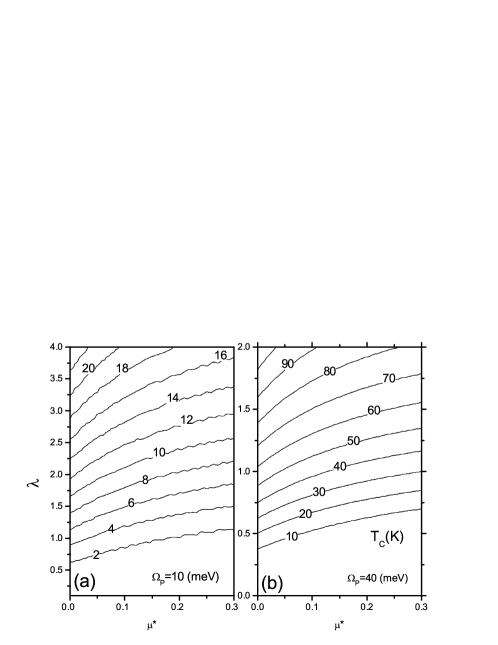
Figure 3: T_c maps in $\mu^{*}-\lambda$ plane with $\Omega_{P}$=10 meV (a) and 40 meV (b).

To study effects of Coulomb pseudo-potential $\mu^{*}$, we calculate two others T_c maps in $\mu^{*}-\lambda$ plane with mesh-grid 50$\times$50 for two phonon energies $\Omega_{P}$=10 meV and 40 meV respectively (Fig.3). For $\Omega_{P}$=10 meV, the maximum of T_c is about 24 K, however 100 K for $\Omega_{P}$=40 meV. We can find that when $\mu^{*}>$ 0.2, $\mu^{*}$ have smaller influences on T_c.

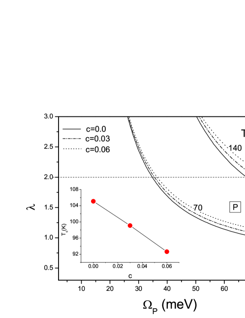
Figure 4: The effects of vertex correlations on T_c map ($\mu^{*}$=0.10) with two parameters c=0.12(eV)/E_F=0.03 and 0.06 compared with the results without vertex corrections c=0.0 (E${}_{F}=\infty$). Two groups of contour lines with T_c=70K and 140K are ploted for three values of c=0.0, 0.03 and 0.06 respectively. The inserted figure plots the curve of T_c by c at a fixed point $P$ shown on the $\lambda-\Omega_{P}$ plane.

4 T_c Map with vertex corrections

It is very important to study the vertex correction in general strong coupling theory  [10]. We control the vertex correction by changing the Fermi-energy $E_{F}$ in the parameter $a_{n}=(2/\pi)\arctan(E_{F}/Z_{n}|\omega_{n}|)$. We choose two values 1.0 eV and 2.0 eV of $E_{F}$. If E_F is too large ($\gg$ 2 eV) the vertex corrections are invisible in our calculations. Two groups of contour lines with T_c=70 K and 140 K are plotted, and for each of groups, there are three contour lines for c=0.0, 0.03 and 0.06 respectively, where c=0.12(eV)/E_F is the control parameter of vertex correction, especially c=0 or E${}_{F}=\infty$ is corresponding to the absence of vertex corrections. We can see that for two T_c, the vertex corrections are so small that the T_c map has no significant changes. For the same T_c, the contour lines only move to regions with larger $\lambda$ slightly. In the inserted figure of Fig.4, at a point $P$ with fixed $\lambda$=1.50 and $\Omega_{P}$=65meV, the vertex corrections decrease T_c to smaller value. However, the negative vertex corrections only happen when $\Omega_{P}<$80 meV and $\lambda<$4. Beyond the ranges of parameters, such as $\Omega_{P}$=90 meV and $\lambda\geq$3.2, the positive vertex corrections (T_c increases with $\omega_{0}/E_{f}$) are realized (Fig.5). It’s not surprised that, if $\lambda<$3.2, only the general negative vertex-corrections are found although the phonon energy $\Omega_{P}$ is larger that 80 meV (Fig.5). The key point is that, although the effects of vertex corrections are rather complicated, they do not change the T_c maps significantly if E_F isn’t too small.

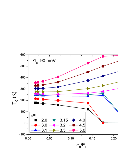
Figure 5: The positive ($\lambda\geq$3.2) and negative vertex corrections ($\lambda<$3.2) at high phonon energy $\Omega_{P}$=90 meV.

We expect that the vertex corrections are strong for superconductors with high T_c. From the Fig.4, we can see that, when $\Omega_{P}$ is smaller than 40 meV, the vertex effect is very small although the parameter $\lambda$ of electron-phonon interaction is probably large. The effect of vertex correction is determined by $\langle\nu^{2}\rangle\lambda$ and not solely by the parameter $\lambda$ of electron-phonon interaction in the region of low phonon-energy. The vertex correction is closely correlated to T_c because of $T_{c}\propto\sqrt{\langle\nu^{2}\rangle\lambda}$ in strong coupling regime with $\lambda>$ 2.0. We will prove that the vertex correction is also characterized by $\langle\nu^{2}\rangle\lambda$ in the region of low phonon energy. It easily sees that the parameter $V_{A}(nn^{\prime})=P_{V}\sum_{m}\lambda(\nu_{m})s_{n^{\prime}-m}s_{n-m}a_{n^{\prime}-m}a_{n-m}$ where $P_{V}=\pi^{2}k_{B}T_{c}/2E_{F}$ and $m=n-n^{\prime\prime}$. If the Einstein spectrum $\alpha^{2}F(\nu)=(\lambda/2)\Omega_{P}\delta(\nu-\Omega_{P})$ is considered, we can get

$$\lambda(\nu_{m})=\lambda\Omega_{P}^{2}/(\nu_{m}^{2}+\Omega_{P}^{2}).$$ (15)

If $\Omega_{P}\rightarrow 0$, then $\lambda(\nu_{m})\rightarrow(1/\nu_{m}^{2})\lambda\Omega_{P}^{2}$, and the parameter of vertex correction $V(nn^{\prime})\rightarrow P_{V}C(n,n^{\prime},T_{c})\lambda\Omega_{P}^{2}$, where $C(n,n^{\prime},T_{c})=\sum_{m}s_{n^{\prime}-m}s_{n-m}a_{n^{\prime}-m}a_{n-m}/\nu_{m}^{2}$ is well defined and finite. So the parameter $\Omega_{P}^{2}\lambda$ or $\langle\nu^{2}\rangle\lambda$ characterizes the vertex correction. In real materials $\Omega_{P}$($\ll E_{F}$) has an up limit $\Omega_{D}$. When $\Omega_{P}$ approaching to high energy, $\lambda(\nu_{m})\rightarrow\lambda\Omega_{D}^{2}/(\nu_{m}^{2}+\Omega_{D}^{2})$, $V(nn^{\prime})\rightarrow P_{V}D(n,n^{\prime},T_{c})\lambda$, where $D(n,n^{\prime},T_{c})=\sum_{m}s_{n^{\prime}-m}s_{n-m}a_{n^{\prime}-m}a_{n-m}\Omega_{D}^{2}/(\nu_{m}^{2}+\Omega_{D}^{2})$ is well defined. So we can see that the vertex correction is characterized by $\lambda$ at high energy. From the Fig.2, T_c is almost independent on $\Omega_{P}$ when $\Omega_{P}>$ 40 meV and $\lambda<2.0$, and T_c is determined by $\lambda$ as well. Thus, we have proven that the vertex correction (as well as T_c) is characterized by $\langle\nu^{2}\rangle\lambda$ in the region of low phonon energy and by $\lambda$ in the region of high phonon energy. There is a characteristic energy close to 40 meV and the vertex corrections (as well as T_c) have different behavior when $\Omega_{P}$ is larger or smaller than the characteristic energy.

5 Discussion and Summary

For superconductors with T_c close to home temperature, the parameter $\lambda$ of electron-phonon interaction should be larger than 2.0 or the phonon-energy $\Omega_{P}$ larger than 80 meV (Fig. 2). Generally, we hope to find higher T_c by increasing the frequency of phonon by choosing compounds including light atoms such as Hydrogen atoms in molecule crystals [21]. The contour line T_c=300K in Fig.2 is beneath the line of $\lambda=$2.0 when $\Omega_{P}$ is larger than 150 meV or 1210 cm^-1 for Raman shift. We can see that only small changes of $\lambda$ can induce large changes of T_c if $\Omega_{P}>$ 80 meV. In compounds with components of light atoms and heavy atoms, the frequencies of optical modes are determined by light atoms. The heavy atoms have the capability to stabilize the lattice vibrations so it is advantaged to form macroscopic-coherent superconducting states.

It is very interesting that we can explain the spatial anti-correlation between energy-gap and phonon energy of cuprate superconductor Bi2212 [22] in terms of the electron-phonon mechanism by having solved the real-energy Eliashberg Equation under the constraint from Eq.(14) [23]. The large value of $\lambda$ ($>$1.0) can be obtained from the frozen-phonon method by considering nonlocal long-range Madelung interaction which is non-adiabatic effect when an atom displaces away from its equilibrium position  [24, 25]. Our results in this context also indicate that the vertex corrections which include part of non-adiabatic effect are closely correlated to high T_c. On the other hand, in terms of the linear temperature-dependent resistivity at high temperature above T_c, the strong electron-phonon coupling could be extracted by the analysis of strong coupling theory [26, 27]. The upper limit of phonon energies of in-plane breathing modes of cuprate superconductors is close to $\Omega_{P}$=80 meV [28]. If the anisotropy of Bi2212 crystal is ignored, from the Fig.1, we can see that the maximum of T_c will be within 140K-160K. The highest T_c is about 130 K for cuprate superconductors close to the range. From the Fig.4, there are larger vertex corrections at higher $\Omega_{P}$ and larger $\lambda$, however the T_c doesn’t changes significantly because the band-width of CuO₂ plane for cuprate superconductors such as Bi2212 is not too small about 4 eV, and the Fermi-energy $E_{F}$ is at least 1 eV [29, 30].

Finally, we discuss the new iron-based layered high-temperature superconductors  [11, 12, 13, 14, 15]. The carriers are mostly possible in FeAs layers. The multi-band electronic structure, especially the cooper-pairs spanning different Fermi-surface sheets probably play an important role to its superconductivity. The pairing mechanism of different Fermi-surface sheets is absent in present model, but the model is still equivalent to the mean of multi-band model. Very similar to the cuprate superconductors, the linear-response calculation of electron-phonon interaction only provides very small parameter $\lambda$ of electron-phonon coupling that does not account the requirement of high T_c from 27(K) to 57(K) [31]. However, just like for cuprate superconductors [25], the nonlocal long-range Madelung interaction generally enhances parameter $\lambda$ of electron-phonon interaction and account the requirements for high T_c. Experimental evidence for strong electron-phonon coupling comes from the measurement of normal-state resistivity at high temperature [32]. The upper limit of phonon-energy is about 40 meV [33]. From the Fig.2 and Fig.3(b), we can predict that the maximum of transition temperature T_c for layered iron-based superconductors may access to 90(K).

In summary, we calculate T_c maps in full parameter space using strong coupling theory including vertex corrections. We also discuss the possibility increasing T_c by using materials including light atoms with higher phonon frequency. The strong vertex corrections are inevitable in materials with high T_c. Based on the maps obtained in this work, we predict the maximum of T_c of new finding iron-based superconductors is about 90(K).

6 Acknowledgement

The author gratefully thanks Dr. Li Yang-Ling for reading and criticizing the manuscript. This work is supported by Director Grants of Hefei Institutes of Physical Sciences, Knowledge Innovation Program of Chinese Academy of Sciences and National Science Foundation of China. The eigenvalues of kernel matrix are obtained by using the Lapack package.

References

- [1] N. W. Ashcroft, Physica C 468 (2008) 115; W. E. Pickett, Physica C 468 (2008) 126; all other papers in Room Temperature Superconductivity edited by B. Jankó, G. W. Crabtree and W. K. Kwok, Physica C 468, issue 2 (2008).
- [2] J. Bardeen, L. N. Cooper, and J. R. Schrieffer, Phys. Rev. 108 (1957) 1175.
- [3] G. M. Éliashberg, Soviet. Phys. JETP, 11 (1960) 696.
- [4] Y. Nambu, Phys. Rev. 117 (1960) 648.
- [5] P. B. Allen, and R. C. Dynes, Phys. Rev. B 12 (1975) 905.
- [6] D. J. Scalapino, J. R. Schrieffer, and J. W. Wilkins, Phys. Rev. 148 (1966) 263.
- [7] W. L. McMillan, Phys. Rev. 167 (1968) 331.
- [8] J. E. Moussa, and M. L. Cohen, Phys. Rev. B 74 (2006) 094520.
- [9] O. V. Dolgov, D. A. Kirzhnits, and E. G. Maksimov, Rev. Mod. Phys. 53 (1981) 81.
- [10] V. N. Kostur and B. Mitrović, Phys. Rev. B 50 (1994) 12774.
- [11] Y. Kamihara, T. Watanabe, M. Hirano, and H. Hosono, J. AM. Chem. Soc. 130 (2008) 3296.
- [12] X. H. Chen, T. Wu, G. Wu, R. H. Liu, H. Chen, D. F. Fang, Nature 453 (2008) 761.
- [13] Z. A. Ren, J. Yang, W. Lu, W. Yi, X. L. Shen, Z. C. Li, G. C. Che, X. L. Dong, L. L. Sun, F. Zhou, Z. X. Zhao, Europhys. Lett. 82 (2008) 57002.
- [14] C. Wang, L. J. Li, S. Chi, Z. W. Zhu, Z. Ren, Y. K. Li, Y. T. Wang, X. Lin, Y. K. Luo, S. Jiang, X. F. Xu, G. H. Cao, and Z. A. Xu, Europhys. Lett. 83 (2008) 67006.
- [15] P. Cheng, B. Shen, G. Mu, X. Y. Zhu, F. Han, B. Zeng, and H. H. Wen, arXiv: 0812.1192 (2008).
- [16] R. H. Liu, T. Wu, G. Wu, H. Chen, X. F. Wang, Y. L. Xie, J. J. Yin, Y. J. Yan, Q. J. Li, B. C. Shi, W. S. Chu, Z. Y. Wu, and X. H. Chen, arXiv:0810.2694 (2008).
- [17] J. P. Carbotte, Rev. Mod. Phys. 62 (1990) 1027.
- [18] C. P. Moca, and B. Jankó, Physica C 387 (2003) 122.
- [19] M. J. Holcomb, Phys. Rev. B 54 (1996) 6648.
- [20] W. H. Press, S. A. Teukolsky, W. T. Vetterling and B. P. Flannery, Numerical Recipes in Fortran 77, The art of scientific computing, Second Edition, Volume 1 of Fortran Numerical Recipes, chapter 9, (Press Syndicate of the University of Cambridge, 1997).
- [21] M. I. Eremets, I. A. Trojan, S. A. Medvedev, J. S. Tse and Y. Yao, Science 319 (2008) 1506.
- [22] Jinho Lee, K. Fujita, K. McElroy, J. A. Slezak, M. Wang, Y. Aiura, H. Bando, M. Ishikado, T. Masui, Jian-Xin Zhu, A. V. Balatsky, H. Eisaki, S. Uchida, and J. C. Davis, Nature 442 (2006) 546.
- [23] W. Fan, Chinese Physics Letter, 25 (2008) 2217.
- [24] T. Jarlborg, Solid State Communications 71 (1989) 669.
- [25] H. Krakauer, W. E. Pickett, and R. E. Cohen, Phys. Rev. B 47 (1993) 1002.
- [26] R. Zeyher, Phys. Rev. B 44 (1991) 10404.
- [27] I. I. Mazin, O. V. Dolgov, Phys. Rev. B 45 (1992) 2509.
- [28] G. M. Zhao, Phys. Rev. B 75 (2007) 214507.
- [29] H. Krakauer, W. E. Pickett, Phys. Rev. Lett. 60 (1988) 1665.
- [30] H. Lin, S. Sahrakorpi, R. S. Markiewicz, and A. Bansil, Phys. Rev. Lett. 96 (2006) 097001.
- [31] L. Boeri, O. V. Dolgov, and A. A. Golubov, Phys. Rev. Lett. 101 (2008) 026403.
- [32] D. Bhoi, P. Mandal, and P. Choudhury, arXiv:0808.2695 (2008).
- [33] S. Higashitaniguchi, M. Seto, S. Kitao, Y. Kobayashi, M. Saito, R. Masuda, T. Mitsui, Y. Yoda, Y. Kamihara, M. Hirano, and H. Hosono, arXiv:0807.3968 (2008).