Optimum Pilot Overhead in Wireless Communication: A Unified Treatment of Continuous and Block-Fading Channels

Nihar Jindal and Angel Lozano Nihar Jindal is with the University of Minnesota, Minneapolis, MN 55455, USA. His work was partially conducted during a visit to UPF under the sponsorship of Project TEC2006-01428.Angel Lozano is with Universitat Pompeu Fabra (UPF), 08018 Barcelona, Spain. His work is supported by the projects CONSOLIDER-INGENIO 2010 CSD2008-00010 ”COMONSENS” and IRG-224755 ”NetMIMO”.
Abstract

The optimization of the pilot overhead in single-user wireless fading channels is investigated, and the dependence of this overhead on various system parameters of interest (e.g., fading rate, signal-to-noise ratio) is quantified. The achievable pilot-based spectral efficiency is expanded with respect to the fading rate about the no-fading point, which leads to an accurate order expansion for the pilot overhead. This expansion identifies that the pilot overhead, as well as the spectral efficiency penalty with respect to a reference system with genie-aided CSI (channel state information) at the receiver, depend on the square root of the normalized Doppler frequency. Furthermore, it is shown that the widely-used block fading model is only a special case of more accurate continuous fading models in terms of the achievable pilot-based spectral efficiency, and that the overhead optimization for multiantenna systems is effectively the same as for single-antenna systems with the normalized Doppler frequency multiplied by the number of transmit antennas.

I Introduction

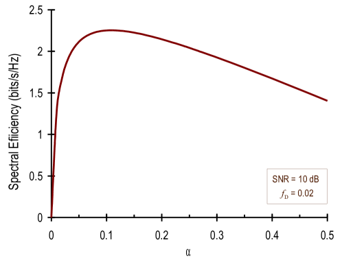
Most wireless communication systems perform coherent data detection with the assistance of pilot signals (a.k.a. reference signals or training sequences) that are inserted periodically [1, 2]. The receiver typically performs channel estimation on the basis of the received pilot symbols, and then applies standard coherent detection while treating the channel estimate as if it were the true channel. When such an approach is taken and Gaussian inputs are used, the channel estimation error effectively introduces additional Gaussian noise [3, 4]. This leads to a non-trivial tradeoff: increasing the fraction of symbols that serve as pilots improves the channel estimation quality and thus decreases this additional noise, but also decreases the fraction of symbols that can carry data. To illustrate the importance of this tradeoff, Fig. 1 depicts the spectral efficiency as function of the pilot overhead (cf. Section III for details) for some standard channel conditions. Clearly, an incorrect overhead can greatly diminish the achievable spectral efficiency.

Although this optimization is critical and has been extensively studied in the literature [3][13], on the basis of both the simplified block-fading model as well as the more accurate continuous-fading model, such optimization must be solved numerically except for one known special case.111A closed-form solution for the optimal overhead when the power of the pilot symbols can be boosted in a block-fading channel model is derived in [6]. Indeed, other than some low- and high-power asymptotes, no explicit expressions are available to identify the optimum overhead or to assess how it depends on the various parameters of interest (velocity, power, etc).

In this paper, we circumvent this difficulty by studying the overhead optimization in the limiting regime of slow fading. More precisely, by expanding the spectral efficiency around the perfect-CSI point, i.e., for small fading rates, the optimization can be tackled and a useful expansion (in terms of the fading rate) for the optimum pilot overhead is obtained. The key insights reached in the paper are as follows:

  • In terms of the spectral efficiency achievable with channel estimate-based decoding, block-fading is simply a special case of continuous (symbol-by-symbol) fading.

  • The optimal pilot overhead scales with the square root of the Doppler frequency; this result holds regardless of whether pilot power boosting is allowed.222To the best of our knowledge, this square-root dependence was first identified in the context of a different (and weaker) lower bound for the multiantenna broadcast channel in [14].

  • The spectral efficiency penalty w.r.t. the perfect-CSI capacity also scales with the square-root of the fading rate.

  • The pilot overhead optimization for multiantenna transmission is essentially the same as the optimization for single-antenna transmission except with the true Doppler frequency multiplied by the number of transmit antennas.

II Preliminaries

A Channel Model

Consider a discrete-time frequency-flat scalar fading channel $H(k)$ where $k$ is the time index. (The extension to multiantenna channels is considered in Section VI.) Pilot symbols are inserted periodically in the transmission [15] and the fraction thereof is denoted by $\alpha$, i.e., one in every $1/\alpha$ symbols is a pilot while the rest are data. Moreover, $\alpha\geq\alpha_{\rm min}$ where $\alpha_{\rm min}$ is established later in this section.

Let $\mathcal{D}$ denote the set of time indices corresponding to data symbols. For $k\in\mathcal{D}$,

$$Y(k)=H(k)\sqrt{P}X(k)+N(k)$$ (1)

where the transmitted signal, $X(k)$, is a sequence of IID (independent identically distributed) complex Gaussian random variables with zero mean and unit variance that we indicate by $X\sim\mathcal{N}_{\mathbb{C}}(0,1)$. The additive noise is $N\sim\mathcal{N}_{\mathbb{C}}(0,N_{0})$ and we define $\mbox{\scriptsize\sf SNR}=P/N_{0}$.

For $k\notin\mathcal{D}$, unit-amplitude pilots are transmitted and thus

$$Y(k)=H(k)\sqrt{P}+N(k).$$ (2)

Notice that pilot symbols and data symbols have the same average power. In Section V, we shall lift this constraint allowing for power-boosted pilots.

A.1 Block Fading

In the popular block-fading model, the channel is drawn as $H\sim\mathcal{N}_{\mathbb{C}}(0,1)$ at the beginning of each block and it then remains constant for the $n_{\sf b}$ symbols composing the block. This process is repeated for every block in an IID fashion.

In order for the receiver to estimate the channel, at least one pilot symbol must be inserted within each block. If $n_{\sf p}$ represents the number of pilot symbols in every block, then

$$\alpha=\frac{n_{\sf p}}{n_{\sf b}}$$ (3)

and clearly $\alpha_{\rm min}=1/n_{\sf b}$.

A.2 Continuous Fading

In this model, $H(k)$ is a discrete-time complex Gaussian stationary333The block-fading model, in contrast, is not stationary but only cyclostationary. random process, with an absolutely continuous spectral distribution function whose derivative is the Doppler spectrum $S_{H}(\nu)$, $-1/2\leq\nu\leq 1/2$. It follows that the channel is ergodic.

The discrete-time process $H(k)$ is derived from an underlying continuous-time fading process whose Doppler spectrum is $S(f)$. We consider bandlimited processes such that

$$\left\{\begin{array}[]{ll}S(f)>0,&\quad|f|\leq f_{\sf m}\\ S(f)=0,&\quad|f|>f_{\sf m}\end{array}\right.$$ (4)

User motion generally results in $f_{\sf m}=v/\lambda$ where $v$ is the velocity and $\lambda$ is the carrier wavelength. (Higher values for $f_{\sf m}$ may result if the reflectors are also in motion or if multiple reflexions take place.)

Denoting by $T$ the symbol period and by $\Pi(\cdot)$ the Fourier transform of the transmission pulse shape, the spectrum of the discrete-time and continuous-time processes are related according to

$$S_{H}(\nu)=\frac{1}{T}\,S\left(\frac{\nu}{T}\right)\Pi^{2}(\nu).$$ (5)

As a result, the discrete-time spectrum is nonzero only for $|\nu|\leq f_{\sf m}T$.444Note that (5) implies a matched-filter front-end at the receiver. This entails no loss of optimality if $f_{\sf m}\ll 1/T$, a premise usually satisfied, and the smooth pulse shaping $\Pi(\cdot)$ can thereby be disregarded altogether. For notational convenience, we therefore define a normalized Doppler $f_{\rm\scriptscriptstyle D}=f_{\sf m}T$.

To ensure that the decimated channel observed through the pilot transmissions has an unaliased spectrum, it is necessary that

$$\alpha_{\sf min}=2f_{\rm\scriptscriptstyle D}.$$ (6)

On account of its bandlimited nature, the channel is a nonregular fading process [16]. For simplicity we further consider $S_{H}(\cdot)$ to be strictly positive within $\pm f_{\rm\scriptscriptstyle D}$.555This premise can be easily removed by simply restricting all the integrals in the paper to the set of frequencies where $S_{H}(\nu)>0$, rather than to the entire interval $\pm f_{\rm\scriptscriptstyle D}$. In order to remain consistent with earlier definitions of signal and noise power, only unit-power processes are considered.

Two important spectra are the Clarke-Jakes [17]

$$S_{H}(\nu)=\frac{1}{\pi\sqrt{f_{\rm\scriptscriptstyle D}^{2}-\nu^{2}}}$$ (7)

and the rectangular

$$S_{H}(\nu)=\left\{\begin{array}[]{ll}1/(2f_{\rm\scriptscriptstyle D})&\quad|\nu|\leq f_{\rm\scriptscriptstyle D}\\ 0&\quad|\nu|>f_{\rm\scriptscriptstyle D}.\end{array}\right.$$ (8)

We will later find it useful to express the Doppler spectrum as

$$S_{H}(\nu)=\frac{1}{f_{\rm\scriptscriptstyle D}}\,\tilde{S}_{H}\!\left(\frac{\nu}{f_{\rm\scriptscriptstyle D}}\right)$$ (9)

where $\tilde{S}_{H}(\cdot)$ is a normalized spectral shape bandlimited to $\pm 1$. For the Clarke-Jakes spectrum in (7), for instance, the spectral shape is

$$\tilde{S}_{H}(\nu)=\frac{1}{\pi\sqrt{1-\nu^{2}}}$$ (10)

while, for the rectangular spectrum in (8), the spectral shape is

$$\tilde{S}_{H}(\nu)=\left\{\begin{array}[]{ll}1/2&\quad|\nu|\leq 1\\ 0&\quad|\nu|>1.\end{array}\right.$$ (11)

B Perfect CSI

With perfect CSI at the receiver, i.e., assuming a genie provides the receiver with $H(k)$, there is no need for pilot symbols ($\alpha=0$). The capacity in bits/s/Hz is then [18, 19]

$\displaystyle C(\mbox{\scriptsize\sf SNR})$ $\displaystyle=$ $\displaystyle E\left[\log_{2}\left(1+\mbox{\scriptsize\sf SNR}\,|H|^{2}\right)\right]$ (12)
$\displaystyle=$ $\displaystyle\log_{2}(e)\;e^{1/\mbox{\scriptsize\sf SNR}}E_{1}\!\left(\frac{1}{\mbox{\scriptsize\sf SNR}}\right)$ (13)

with $E_{q}(\cdot)$ the exponential integral of order $q$,

$$E_{q}(\zeta)=\int_{1}^{\infty}t^{-q}e^{-\zeta t}dt.$$ (14)

The first derivative of $C(\cdot)$ can be conveniently expressed as a function of $C(\cdot)$ via

$$\dot{C}(\mbox{\scriptsize\sf SNR})=\frac{1}{\mbox{\scriptsize\sf SNR}}\left(\log_{2}e-\frac{C(\mbox{\scriptsize\sf SNR})}{\mbox{\scriptsize\sf SNR}}\right).$$ (15)

In turn, the second derivative can be expressed as function of $C(\cdot)$ and $\dot{C}(\cdot)$ as

$$\ddot{C}(\mbox{\scriptsize\sf SNR})=-\frac{1}{\mbox{\scriptsize\sf SNR}^{2}}\left[\log_{2}e+\dot{C}(\mbox{\scriptsize\sf SNR})-2\frac{C(\mbox{\scriptsize\sf SNR})}{\mbox{\scriptsize\sf SNR}}\right].$$ (16)

III Pilot-Assisted Detection

In pilot-assisted communication, decoding must be conducted on the basis of the channel outputs (data and pilots) alone, without the assistance of genie-provided channel realizations. In this case, the maximum spectral efficiency that can be achieved reliably is the mutual information between the data inputs and the outputs (data and pilots). This mutual information equals

$$\lim_{K\rightarrow\infty}\frac{1}{K}\;I\!\left(\underbrace{\{X(k)\}_{k=0}^{K-1};\{Y(k)\}_{k=0}^{K-1}}_{k\in\mathcal{D}}|\underbrace{\{Y(k)\}_{k=0}^{K-1}}_{k\notin\mathcal{D}}\right)$$ (17)

where $K$ signifies the blocklength in symbols. Achieving (17), for which there is no known simplified expression, generally requires joint data decoding and channel estimation.

Contemporary wireless systems take the lower complexity, albeit suboptimal, approach of first estimating the channel for each data symbol—based exclusively upon all received pilot symbols—and then performing nearest-neighbor decoding using these channel estimates as if they were correct. This is an instance of mismatched decoding [20]. If we express the channel as $H(k)=\hat{H}(k)+\tilde{H}(k)$ where $\hat{H}(k)$ denotes the minimum mean-square error estimate of $H(k)$, the received symbol can be re-written as

$$Y(k)=\hat{H}(k)\sqrt{P}\,X(k)+\tilde{H}(k)\sqrt{P}\,X(k)+N(k).$$ (18)

Performing nearest-neighbor decoding as described above666More specifically, the decoder finds the codeword $[X(1),\ldots,X(K)]$ that minimizes the distance metric $\sum_{k=1}^{K}|Y(k)-\sqrt{P}\hat{H}(k)X(k)|^{2}$. has been shown to have the effect of making the term $\tilde{H}(k)\sqrt{P}\,X(k)$ appear as an additional source of independent Gaussian noise [4]. With that, the spectral efficiency becomes [3][11]

$$\bar{\mathcal{I}}(\mbox{\scriptsize\sf SNR},\alpha)=(1-\alpha)\,C(\mbox{\scriptsize\sf SNR}_{\sf eff})$$ (19)

with

$$\mbox{\scriptsize\sf SNR}_{\sf eff}=\frac{\mbox{\scriptsize\sf SNR}\,(1-\mbox{\scriptsize\sf MMSE})}{1+\mbox{\scriptsize\sf SNR}\cdot\mbox{\scriptsize\sf MMSE}}$$ (20)

where $\mbox{\scriptsize\sf MMSE}=E\left[|\tilde{H}|^{2}\right]$. Although not shown explicitly, MMSE and $\mbox{\scriptsize\sf SNR}_{\sf eff}$ are functions of SNR, $\alpha$ and the underlying fading model.

In addition to representing the maximum spectral efficiency achievable with Gaussian codebooks and channel-estimate-based nearest-neighbor decoding, $\bar{\mathcal{I}}(\cdot)$ is also a lower bound to (17). Because of this double significance, the maximization of $\bar{\mathcal{I}}(\cdot)$ over $\alpha$

$$\bar{\mathcal{I}}^{\star}(\mbox{\scriptsize\sf SNR})=\max_{\alpha_{\rm min}\leq\alpha\leq 1}\bar{\mathcal{I}}(\mbox{\scriptsize\sf SNR},\alpha)$$ (21)

and especially the argument of such maximization, $\alpha^{\star}$, are the focal points of this paper.

The expressions in (19) and (21) apply to both block and continuous fading, and these settings differ only in how MMSE behaves as a function of $\alpha$ and SNR.

In block fading, $n_{\sf p}$ pilot symbols are used to estimate the channel in each block and thus [6]

$$\mbox{\scriptsize\sf MMSE}=\frac{1}{1+\alpha\,n_{\sf b}\mbox{\scriptsize\sf SNR}}.$$ (22)

For continuous fading, on the other hand [2, 11]

MMSE $\displaystyle=$ $\displaystyle 1-\int_{-f_{\rm\scriptscriptstyle D}}^{+f_{\rm\scriptscriptstyle D}}\frac{\mbox{\scriptsize\sf SNR}\,S_{H}^{2}(\nu)}{1/\alpha+\mbox{\scriptsize\sf SNR}\,S_{H}(\nu)}\,d\nu$ (23)
$\displaystyle=$ $\displaystyle 1-\int_{1}^{+1}\frac{\tilde{S}_{H}^{2}(\xi)}{\frac{f_{\rm\scriptscriptstyle D}}{\alpha\,\mbox{\scriptsize\sf SNR}}+\tilde{S}_{H}(\xi)}\,d\xi$ (24)

where the latter is derived based upon the spectral shape definition in (9).

For the Clarke-Jakes spectrum, (23) can be computed in closed form as [13]

$$\mbox{\scriptsize\sf MMSE}=1-\frac{{\rm arctanh}\sqrt{1-\left(\frac{\alpha\,\scriptscriptstyle\sf SNR}{\pi f_{\rm\scriptscriptstyle D}}\right)^{2}}}{\frac{\pi}{2}\sqrt{\left(\frac{\pi f_{\rm\scriptscriptstyle D}}{\alpha\,{\scriptscriptstyle\sf SNR}}\right)^{2}-1}}$$ (25)

while, for the rectangular spectrum [11]

$$\mbox{\scriptsize\sf MMSE}=\frac{1}{1+\frac{\alpha}{2f_{\rm\scriptscriptstyle D}}\mbox{\scriptsize\sf SNR}}.$$ (26)

Comparing (22) with (26), the block-fading model is seen to yield the same MMSE as a continuous fading model with a rectangular spectrum where

$$f_{\rm\scriptscriptstyle D}=\frac{1}{2n_{\sf b}}.$$ (27)

Because $\bar{\mathcal{I}}(\cdot)$ depends on the fading model only through MMSE, this further implies equivalence in terms of spectral efficiency. Thus, for the remainder of the paper we shall consider only continuous fading while keeping in mind that block-fading corresponds to the special case of a rectangular spectrum with (27).

IV Pilot Overhead Optimization

The optimization in (21) does not yield an analytical solution, even for the simplest of fading models, and therefore it must be computed numerically.777Such numerical computation is further complicated by the fact that for most spectra other than Clarke-Jakes and rectangular, a closed-form solution for MMSE does not even exist. In this section, we circumvent this difficulty by appropriately expanding the objective function $\bar{\mathcal{I}}(\cdot)$. This leads to a simple expression that cleanly illustrates the dependence of $\alpha^{*}$ and $\bar{\mathcal{I}}^{*}$ on the parameters of interest.

In particular, we shall expand (19) with respect to $f_{\rm\scriptscriptstyle D}$ while keeping the shape of the Doppler spectrum fixed (but arbitrary). Besides being analytically convenient, this approach correctly models different velocities within a given propagation environment.888The propagation environment determines the shape of the spectrum while the velocity and the symbol time determine $f_{\rm\scriptscriptstyle D}$. We shall henceforth explicitly show the dependence of $\bar{\mathcal{I}}(\cdot)$ and $\bar{\mathcal{I}}^{\star}(\cdot)$ on $f_{\rm\scriptscriptstyle D}$. In addition, we recall the notion of spectral shape $\tilde{S}_{H}(\cdot)$ introduced in (9) and, for the sake of compactness, we introduce the notation

$$\left[z\right]_{a}^{b}=\left\{\begin{array}[]{ll}a&z\leq a\\ z&a<z<b\\ b&z\geq b\end{array}\right.$$ (28)
Proposition 1

The optimum pilot overhead for a Rayleigh-faded channel with an arbitrary bandlimited Doppler spectrum is given by

$\displaystyle\alpha^{\star}$ $\displaystyle=$ $\displaystyle\left[\sqrt{(1+\mbox{\scriptsize\sf SNR})\,\frac{\dot{C}(\mbox{\scriptsize\sf SNR})}{C(\mbox{\scriptsize\sf SNR})}\,2f_{\rm\scriptscriptstyle D}}\right.$ (29)
$\displaystyle\left.-\left((1+\mbox{\scriptsize\sf SNR})\,\frac{\ddot{C}(\mbox{\scriptsize\sf SNR})}{\dot{C}(\mbox{\scriptsize\sf SNR})}+2+\frac{1}{2\,\mbox{\scriptsize\sf SNR}}\int_{-1}^{+1}\frac{d\xi}{\tilde{S}_{H}(\xi)}\right)f_{\rm\scriptscriptstyle D}\right]_{2f_{\rm\scriptscriptstyle D}}^{1}\!\!\!\!\!\!\!+\mathcal{O}(f_{\rm\scriptscriptstyle D}^{3/2}).$

Proof: See Appendix A.

The expression for $\alpha^{\star}$ in Proposition 1 is a simple function involving the perfect-CSI capacity and its derivatives (cf. Section II). Furthermore, the leading term in the expansion does not depend on the particular spectral shape. Only the subsequent term begins to exhibit such dependence, through $\int_{-1}^{+1}d\nu/\tilde{S}_{H}(\nu)$. For a Clarke-Jakes spectrum, for instance, this integral equals $\pi^{2}/2$. For a rectangular spectrum, it equals $4$.

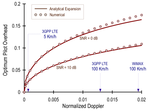
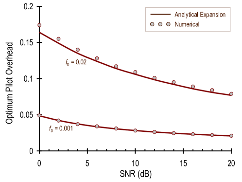
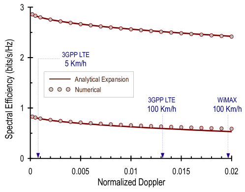
Comparisons between the optimum pilot overhead given by Proposition 1 and the corresponding exact value obtained numerically are presented in Figs. 23. The agreement is excellent for essentially the entire range of Doppler and SNR values of interest in mobile wireless systems.

Once the overhead has been optimized, the corresponding spectral efficiency is given, from (19) and Proposition 1, by

$$\bar{\mathcal{I}}^{\star}(\mbox{\scriptsize\sf SNR},f_{\rm\scriptscriptstyle D})=C\left(\mbox{\scriptsize\sf SNR}\right)-\sqrt{8f_{\rm\scriptscriptstyle D}\left(1+\mbox{\scriptsize\sf SNR}\right)C\left(\mbox{\scriptsize\sf SNR}\right)\dot{C}\left(\mbox{\scriptsize\sf SNR}\right)}+\mathcal{O}(f_{\rm\scriptscriptstyle D})$$ (30)

when $\alpha^{\star}>2f_{\rm\scriptscriptstyle D}$ (up to the order of the expansion). Otherwise,

$$\bar{\mathcal{I}}^{\star}(\mbox{\scriptsize\sf SNR},f_{\rm\scriptscriptstyle D})=(1-2f_{\rm\scriptscriptstyle D})\;C\!\left(\frac{\mbox{\scriptsize\sf SNR}-1}{2}\right)+\mathcal{O}(f_{\rm\scriptscriptstyle D}^{2}).$$ (31)

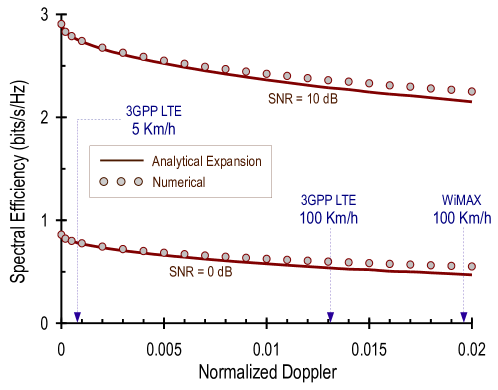
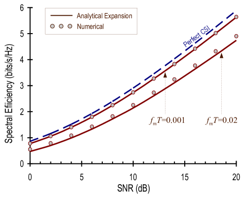
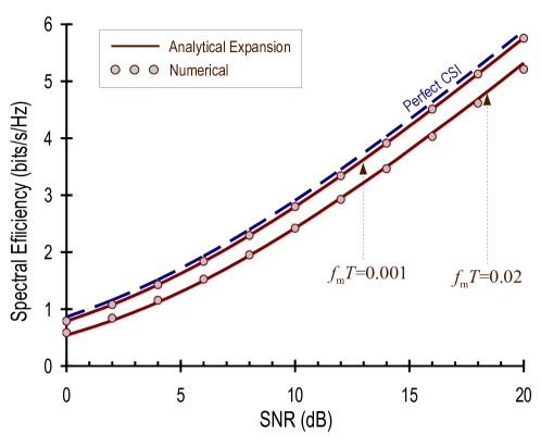
As with the optimum overhead, good agreement is shown in Figs. 45 between the spectral efficiency in (30) and its numerical counterpart as rendered by (21).

A direct insight of Proposition 1 is that the optimum pilot overhead, $\alpha^{*}$, and the spectral efficiency penalty w.r.t. the perfect-CSI capacity, $C(\mbox{\scriptsize\sf SNR})-\bar{\mathcal{I}}^{\star}(\mbox{\scriptsize\sf SNR},f_{\rm\scriptscriptstyle D})$, both depend on the Doppler as $\sqrt{f_{\rm\scriptscriptstyle D}}$. To gain an intuitive understanding of this scaling, we can express such penalty for an arbitrary $\alpha$ as (cf. Appendix A, Eq. A)

$$C(\mbox{\scriptsize\sf SNR})-\bar{\mathcal{I}}(\mbox{\scriptsize\sf SNR},\alpha,f_{\rm\scriptscriptstyle D})=\alpha\,C(\mbox{\scriptsize\sf SNR})+\frac{(1+\mbox{\scriptsize\sf SNR})\dot{C}(\mbox{\scriptsize\sf SNR})\,2f_{\rm\scriptscriptstyle D}}{\alpha}+\mathcal{O}(f_{\rm\scriptscriptstyle D}).$$ (32)

The first term in (32) represents the spectral efficiency loss because only a fraction $(1-\alpha)$ of the symbols contain data, while the second term is the loss on those transmitted data symbols due to the inaccurate CSI. If $\alpha$ is chosen to be $\mathcal{O}(f_{\rm\scriptscriptstyle D}^{s})$ for $0\leq s\leq 1$, the first and second terms in (32) are $\mathcal{O}(f_{\rm\scriptscriptstyle D}^{s})$ and $\mathcal{O}(f_{\rm\scriptscriptstyle D}^{1-s})$, respectively, and thus the overall penalty is

$$\mathcal{O}\left(f_{\rm\scriptscriptstyle D}^{\min\{s,1-s\}}\right).$$ (33)

Hence, the spectral efficiency penalty is minimized by balancing the two terms and selecting $\alpha^{\star}=\mathcal{O}(\sqrt{f_{\rm\scriptscriptstyle D}})$.

In parsing the dependence of $\alpha^{\star}$ upon SNR, it is worth noting that $(1+\mbox{\scriptsize\sf SNR})\,\dot{C}(\mbox{\scriptsize\sf SNR})/C(\mbox{\scriptsize\sf SNR})$ is very well approximated by $1/\log_{e}(1+\mbox{\scriptsize\sf SNR})$. Thus, the optimal overhead decreases with SNR approximately as $1/\sqrt{\log_{e}(1+\mbox{\scriptsize\sf SNR})}$. However, it is important to realize that, although our expansion is remarkably accurate for a wide range of SNR values, it becomes less accurate for $\mbox{\scriptsize\sf SNR}\rightarrow 0$ or $\mbox{\scriptsize\sf SNR}\rightarrow\infty$. In fact, in limiting SNR regimes it is possible to explicitly handle arbitrary Doppler levels [5, 6, 12, 13]. Thus, it is precisely for intermediate SNR values where the analysis here is both most accurate and most useful, thereby complementing those in the aforegiven references.

V Pilot Power Boosting

In some systems, it is possible to allocate unequal powers for pilot and data symbols. Indeed, most emerging wireless systems feature some degree of pilot power boosting [21, 22]. In our models, this can be accommodated by defining the signal-to-noise ratios for pilot and data symbols to be $\rho_{\sf p}\mbox{\scriptsize\sf SNR}$ and $\rho_{\sf d}\mbox{\scriptsize\sf SNR}$, respectively, with

$$\rho_{\sf p}\alpha+\rho_{\sf d}(1-\alpha)=1.$$ (34)

Eq. (19) continues to hold, only with

$$\mbox{\scriptsize\sf SNR}_{\sf eff}=\frac{\mbox{\scriptsize\sf SNR}\,(1-\mbox{\scriptsize\sf MMSE})}{1/\rho_{\sf d}+\mbox{\scriptsize\sf SNR}\cdot\mbox{\scriptsize\sf MMSE}}.$$ (35)

The expressions for MMSE in (22) and (23) hold with SNR replaced with $\rho_{\sf p}\mbox{\scriptsize\sf SNR}$. As a result, with block fading,

$$\mbox{\scriptsize\sf MMSE}=\frac{1}{1+\alpha\,n_{\sf b}\,\rho_{\sf p}\mbox{\scriptsize\sf SNR}}$$ (36)

while, with continuous fading,

$$\mbox{\scriptsize\sf MMSE}=1-\int_{-f_{\rm\scriptscriptstyle D}}^{+f_{\rm\scriptscriptstyle D}}\frac{\mbox{\scriptsize\sf SNR}\,S_{H}^{2}(\nu)}{1/(\rho_{\sf p}\alpha)+\mbox{\scriptsize\sf SNR}\,S_{H}(\nu)}\,d\nu.$$ (37)

It is easily verified, from (36) and (37), that the identity between block fading and continuous fading with a rectangular Doppler spectrum continues to hold under condition (27). In turn, for a Clarke-Jakes spectrum, (37) gives [13]

$$\mbox{\scriptsize\sf MMSE}=1-\frac{{\rm arctanh}\sqrt{1-\left(\frac{\rho_{\sf p}{\scriptscriptstyle\sf SNR}}{\pi/2}\right)^{2}}}{\frac{\pi}{2}\sqrt{\left(\frac{\pi/2}{\rho_{\sf p}{\scriptscriptstyle\sf SNR}}\right)^{2}-1}}.$$ (38)

It can be inferred, from (19), (35) and (37), that it is advantageous to increase $\rho_{\sf p}$ while simultaneously reducing $\alpha$ all the way to $\alpha_{\sf min}$. Indeed, for the block-fading model, the observation is made in [5, 6, 8] that, with pilot power boosting, a single pilot symbol should be inserted on every fading block. With continuous fading, that translates to

$$\alpha=2f_{\rm\scriptscriptstyle D}$$ (39)

and the issue is then the optimization of $\rho_{\sf p}$ and $\rho_{\sf d}$. With $\alpha$ fixed, moreover, the power boosting that maximizes $\bar{\mathcal{I}}(\cdot)$ is directly the one that maximizes $\mbox{\scriptsize\sf SNR}_{\sf eff}$, i.e.,

$$\rho_{\sf p}^{\star}={\rm arg}\max_{\rho_{\sf p}\alpha_{\sf min}+\rho_{\sf d}(1-\alpha_{\sf min})=1}\mbox{\scriptsize\sf SNR}_{\sf eff}$$ (40)

Although simpler than the optimization in Section IV, this nonetheless must be computed numerically, with the exception of the rectangular spectra/block-fading [6, Theorem 2].

As in Section III, we circumvent this limitation by expanding the problem in $f_{\rm\scriptscriptstyle D}$. Again, this yields expressions that are explicit and valid for arbitrary spectral shapes.

Proposition 2

The optimum power allocation for a Rayleigh-faded channel with an arbitrary bandlimited Doppler spectrum is given by

$\displaystyle\rho_{\sf p}^{\star}$ $\displaystyle=$ $\displaystyle\sqrt{\frac{1+1/\mbox{\scriptsize\sf SNR}}{2f_{\rm\scriptscriptstyle D}}}+\mathcal{O}(1)$ (41)
$\displaystyle\rho_{\sf d}^{\star}$ $\displaystyle=$ $\displaystyle 1-\sqrt{\left(1+\frac{1}{\mbox{\scriptsize\sf SNR}}\right)2f_{\rm\scriptscriptstyle D}}+\mathcal{O}(f_{\rm\scriptscriptstyle D}).$ (42)

Proof: See Appendix B.

As expected, an order expansion of the closed-form solution for the rectangular spectra [6, Theorem 2] matches the above proposition.

As a by-product of Proposition 2, the combination of the expansion of $\mbox{\scriptsize\sf SNR}_{\sf eff}$ with (19) and with (41)–(42) leads to

$$\bar{\mathcal{I}}^{\star}(\mbox{\scriptsize\sf SNR},f_{\rm\scriptscriptstyle D})=C\left(\mbox{\scriptsize\sf SNR}\right)-\sqrt{8f_{\rm\scriptscriptstyle D}\,\mbox{\scriptsize\sf SNR}\,(1+\mbox{\scriptsize\sf SNR})}\,\dot{C}(\mbox{\scriptsize\sf SNR})+\mathcal{O}(f_{\rm\scriptscriptstyle D}).$$ (43)

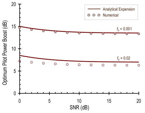
A comparison between the optimum pilot power boost given by (41) and the corresponding value obtained numerically is presented in Fig. 6. The agreement is excellent. Good agreement is further shown in Figs. 78 between the corresponding spectral efficiency in (43) and its exact counterpart, again obtained numerically.

While $\alpha$ is a direct measure of the pilot overhead in terms of bandwidth, the overhead in terms of power is measured by the product $\rho_{\sf p}\alpha$, which signifies the fraction of total transmit power devoted to pilot symbols. In light of (39) and Proposition 2, the optimum pilot power fraction when boosting is allowed equals

$$\rho_{\sf p}^{\star}\alpha=\sqrt{\left(1+\frac{1}{\mbox{\scriptsize\sf SNR}}\right)2f_{\rm\scriptscriptstyle D}}+\mathcal{O}(f_{\rm\scriptscriptstyle D})$$ (44)

while without boosting (i.e., with $\rho_{\sf p}=1$) the pilot power fraction is (from Proposition 1)

$$\alpha^{\star}=\sqrt{(1+\mbox{\scriptsize\sf SNR})\,\frac{\dot{C}(\mbox{\scriptsize\sf SNR})}{C(\mbox{\scriptsize\sf SNR})}\,2f_{\rm\scriptscriptstyle D}}+\mathcal{O}(f_{\rm\scriptscriptstyle D}).$$ (45)

In both cases the fraction of pilot power fraction is $\mathcal{O}(\sqrt{f_{\rm\scriptscriptstyle D}})$. Comparing the two, the pilot power fraction with boosting is larger than the fraction without boosting by a factor

$$\sqrt{\frac{C(\mbox{\scriptsize\sf SNR})}{\mbox{\scriptsize\sf SNR}~{}\dot{C}(\mbox{\scriptsize\sf SNR})}}.$$ (46)

This quantity is greater than unity and is increasing in SNR. Since MMSE is a decreasing function of $\rho_{\sf p}\alpha$, this implies that an optimized system with power boosting achieves a smaller MMSE than one without boosting.

Comparing (43) and (30), pilot power boosting increases the spectral efficiency by

$$\sqrt{8f_{\rm\scriptscriptstyle D}(1+\mbox{\scriptsize\sf SNR})\dot{C}(\mbox{\scriptsize\sf SNR})}\left(\sqrt{C(\mbox{\scriptsize\sf SNR})}-\sqrt{\mbox{\scriptsize\sf SNR}\,\dot{C}(\mbox{\scriptsize\sf SNR})}\right)+\mathcal{O}(f_{\rm\scriptscriptstyle D})$$ (47)

which is vanishing for $\mbox{\scriptsize\sf SNR}\rightarrow 0$ and increases monotonically with SNR.

VI Multiantenna Channels

The analysis extends to multiantenna settings in a straightforward manner when there is no antenna correlation. Letting $n_{\mathrm{\scriptscriptstyle T}}$ and $n_{\mathrm{\scriptscriptstyle R}}$ denote the number of transmit and receive antennas, respectively, the channel at time $k$ is now denoted by the $n_{\mathrm{\scriptscriptstyle R}}\times n_{\mathrm{\scriptscriptstyle T}}$ matrix ${\bf H}(k)$. Each of the $n_{\mathrm{\scriptscriptstyle T}}n_{\mathrm{\scriptscriptstyle R}}$ entries of the matrix varies in an independent manner according to the models described in Section II, for either block or continuous fading. The equivalence between block and continuous fading as per (27) extends to this multiantenna setting, and thus we again restrict our discussion to continuous fading.

We denote the perfect-CSI capacity as

$$C_{n_{\mathrm{\scriptscriptstyle T}},n_{\mathrm{\scriptscriptstyle R}}}(\mbox{\scriptsize\sf SNR})={\mathbb{E}}\left[\log_{2}{\rm det}\left({\bf I}+\frac{\mbox{\scriptsize\sf SNR}}{n_{\mathrm{\scriptscriptstyle T}}}{\bf H}{\bf H}^{\dagger}\right)\right],$$ (48)

for which a closed-form expression in terms of the exponential integral can be found in [23].

The spectral efficiency with pilot-assisted detection now becomes

$$\bar{\mathcal{I}}(\mbox{\scriptsize\sf SNR},\alpha)=(1-\alpha)\,C_{n_{\mathrm{\scriptscriptstyle T}},n_{\mathrm{\scriptscriptstyle R}}}(\mbox{\scriptsize\sf SNR}_{\sf eff})$$ (49)

with

$$\mbox{\scriptsize\sf SNR}_{\sf eff}=\frac{\mbox{\scriptsize\sf SNR}\,(1-\mbox{\scriptsize\sf MMSE})}{1+\mbox{\scriptsize\sf SNR}\cdot\mbox{\scriptsize\sf MMSE}}$$ (50)

where MMSE is the estimation error for each entry of the channel matrix ${\bf H}$. This error is minimized by transmitting orthogonal pilot sequences from the various transmit antennas [6], e.g., transmitting a pilot symbol from a single antenna at a time. A pilot overhead of $\alpha$ thus corresponds to a fraction $\frac{\alpha}{n_{\mathrm{\scriptscriptstyle T}}}$ of symbols serving as pilots for a particular transmit antenna (i.e., for the $n_{\mathrm{\scriptscriptstyle R}}$ matrix entries associated with that transmit antenna). As a result, the per-entry MMSE is the same as the single-antenna expression in (24) only with $\alpha$ replaced by $\alpha/n_{\mathrm{\scriptscriptstyle T}}$, i.e.,

$$\mbox{\scriptsize\sf MMSE}=1-\int_{1}^{+1}\frac{\tilde{S}_{H}^{2}(\xi)}{\frac{n_{\mathrm{\scriptscriptstyle T}}f_{\rm\scriptscriptstyle D}}{\alpha\,\mbox{\scriptsize\sf SNR}}+\tilde{S}_{H}(\xi)}\,d\xi.$$ (51)

This equals the MMSE for a single-antenna channel with a Doppler frequency of $n_{\mathrm{\scriptscriptstyle T}}f_{\rm\scriptscriptstyle D}$. The optimization w.r.t. $\alpha$ in a multiantenna channel is thus the same as in a single-antenna channel, only with an effective Doppler frequency of $n_{\mathrm{\scriptscriptstyle T}}f_{\rm\scriptscriptstyle D}$ and with the function $C(\mbox{\scriptsize\sf SNR})$ replaced by $C_{n_{\mathrm{\scriptscriptstyle T}},n_{\mathrm{\scriptscriptstyle R}}}(\mbox{\scriptsize\sf SNR})$. As a result, Proposition 1 naturally extends into

$\displaystyle\alpha^{\star}$ $\displaystyle=$ $\displaystyle\left[\sqrt{(1+\mbox{\scriptsize\sf SNR})\,\frac{\dot{C}_{n_{\mathrm{\scriptscriptstyle T}},n_{\mathrm{\scriptscriptstyle R}}}(\mbox{\scriptsize\sf SNR})}{C_{n_{\mathrm{\scriptscriptstyle T}},n_{\mathrm{\scriptscriptstyle R}}}(\mbox{\scriptsize\sf SNR})}\,2n_{\mathrm{\scriptscriptstyle T}}f_{\rm\scriptscriptstyle D}}\right.$ (52)
$\displaystyle\left.-\left((1+\mbox{\scriptsize\sf SNR})\,\frac{\ddot{C}_{n_{\mathrm{\scriptscriptstyle T}},n_{\mathrm{\scriptscriptstyle R}}}(\mbox{\scriptsize\sf SNR})}{\dot{C}_{n_{\mathrm{\scriptscriptstyle T}},n_{\mathrm{\scriptscriptstyle R}}}(\mbox{\scriptsize\sf SNR})}+2+\frac{1}{2\,\mbox{\scriptsize\sf SNR}}\int_{-1}^{+1}\frac{d\xi}{\tilde{S}_{H}(\xi)}\right)n_{\mathrm{\scriptscriptstyle T}}f_{\rm\scriptscriptstyle D}\right]_{2n_{\mathrm{\scriptscriptstyle T}}f_{\rm\scriptscriptstyle D}}^{1}\!\!\!\!\!\!\!+\mathcal{O}(f_{\rm\scriptscriptstyle D}^{3/2}).$

Notice here the dependence on $\sqrt{n_{\mathrm{\scriptscriptstyle T}}}$ in the leading term.

When pilot power boosting is allowed, it is again advantageous to reduce $\alpha$ to its minimum value, now given by $\alpha_{\sf min}=2n_{\mathrm{\scriptscriptstyle T}}f_{\rm\scriptscriptstyle D}$, and to increase $\rho_{\sf p}$. In this case the achievable spectral efficiency becomes

$$(1-2n_{\mathrm{\scriptscriptstyle T}}f_{\rm\scriptscriptstyle D})\,C_{n_{\mathrm{\scriptscriptstyle T}},n_{\mathrm{\scriptscriptstyle R}}}(\mbox{\scriptsize\sf SNR}_{\sf eff})$$ (53)

with $\mbox{\scriptsize\sf SNR}_{\sf eff}$ as defined in (20) and with

$$\mbox{\scriptsize\sf MMSE}=1-\int_{1}^{+1}\frac{\tilde{S}_{H}^{2}(\xi)}{\frac{n_{\mathrm{\scriptscriptstyle T}}f_{\rm\scriptscriptstyle D}}{\alpha\,\rho_{\sf p}\,\mbox{\scriptsize\sf SNR}}+\tilde{S}_{H}(\xi)}\,d\xi.$$ (54)

The optimization of the power boost again corresponds to the maximization of $\mbox{\scriptsize\sf SNR}_{\sf eff}$ with respect to $\rho_{\sf p}$. Since MMSE is the same as for a single-antenna channel with effective Doppler $n_{\mathrm{\scriptscriptstyle T}}f_{\rm\scriptscriptstyle D}$, the optimum pilot power boost for a multiantenna channel with Doppler frequency $f_{\rm\scriptscriptstyle D}$ is exactly the same as the optimum pilot power boost for a single-antenna channel with the same spectral shape and with Doppler frequency $n_{\mathrm{\scriptscriptstyle T}}f_{\rm\scriptscriptstyle D}$. As a result, the expressions in Section V apply verbatim if $f_{\rm\scriptscriptstyle D}$ is replaced by $n_{\mathrm{\scriptscriptstyle T}}f_{\rm\scriptscriptstyle D}$.

Applying (44), the fraction of power devoted to pilots is given by

$$\rho_{\sf p}^{\star}\alpha=\sqrt{\left(1+\frac{1}{\mbox{\scriptsize\sf SNR}}\right)2n_{\mathrm{\scriptscriptstyle T}}f_{\rm\scriptscriptstyle D}}+\mathcal{O}(f_{\rm\scriptscriptstyle D})$$ (55)

which increases with $\sqrt{n_{\mathrm{\scriptscriptstyle T}}}$.

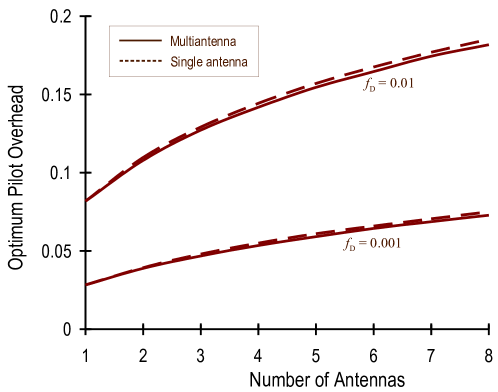
Based upon these results, the pilot overhead optimization on a multiantenna channel with Doppler frequency $f_{\rm\scriptscriptstyle D}$ and a particular spectral shape is effectively equivalent to the optimization on a single-antenna channel with the same spectral shape and with Doppler frequency $n_{\mathrm{\scriptscriptstyle T}}f_{\rm\scriptscriptstyle D}$. When pilot power boosting is allowed, this equivalence is in fact exact. The equivalence is not exact when power boosting is not allowed only because the perfect-CSI capacity functions $C(\mbox{\scriptsize\sf SNR})$ and $C_{n_{\mathrm{\scriptscriptstyle T}},n_{\mathrm{\scriptscriptstyle R}}}(\mbox{\scriptsize\sf SNR})$ differ. Roughly speaking, multiple antennas increase the perfect-CSI capacity by a factor of $\min(n_{\mathrm{\scriptscriptstyle T}},n_{\mathrm{\scriptscriptstyle R}})$ and thus $C_{n_{\mathrm{\scriptscriptstyle T}},n_{\mathrm{\scriptscriptstyle R}}}(\mbox{\scriptsize\sf SNR})\approx\min(n_{\mathrm{\scriptscriptstyle T}},n_{\mathrm{\scriptscriptstyle R}})C(\mbox{\scriptsize\sf SNR})$. If this approximation were exact, then the aforementioned equivalence would also be exact. Although the approximation is not exact, it is sufficiently valid, particularly for symmetric ($n_{\mathrm{\scriptscriptstyle T}}=n_{\mathrm{\scriptscriptstyle R}}$) channels, to render the equivalence very accurate also for the case of non-boosted pilots. To illustrate this accuracy, the optimal pilot overhead for a symmetric channel at an SNR of $10$ dB is plotted versus the number of antennas along with the optimal overhead for the single-antenna equivalent (with Doppler $n_{\mathrm{\scriptscriptstyle T}}f_{\rm\scriptscriptstyle D}$) in Fig. 9. Excellent agreement is seen between the two.

The main implication of the equivalence is that, based upon our earlier results quantifying the dependence of the pilot overhead on the Doppler frequency, the optimal overhead (with or without power boosting) scales with the number of antennas proportional to $\sqrt{n_{\mathrm{\scriptscriptstyle T}}}$.

VII Summary

This paper has investigated the problem of pilot overhead optimization in single-user wireless channels. In the context of earlier work, our primary contributions are two-fold.

First, we were able to unify prior work on continuous- and block-fading channels and on single- and multiantenna channels: the commonly used block-fading model was shown to be a special case of the richer set of continuous-fading models in terms of the achievable pilot-based spectral efficiency, and the pilot overhead optimization for multiantenna chanels is seen to essentially be equivalent to the same optimization for a single-antenna channel in which the normalized Doppler frequency is multiplied by the number of transmit antennas.

Second, by finding an expansion for the overhead optimization in terms of the fading rate, the square root dependence of both the overhead and the spectral efficiency penalty was cleanly identified.

Appendices

A Proof of Proposition 1

We set out to expand $\bar{\mathcal{I}}(\mbox{\scriptsize\sf SNR},\alpha)$ w.r.t. $f_{\rm\scriptscriptstyle D}$ about the point $f_{\rm\scriptscriptstyle D}=0$ while holding SNR and $\alpha$ fixed. We need

$\displaystyle\frac{\partial\bar{\mathcal{I}}(\mbox{\scriptsize\sf SNR},\alpha,f_{\rm\scriptscriptstyle D})}{\partial f_{\rm\scriptscriptstyle D}}|_{f_{\rm\scriptscriptstyle D}=0}$ $\displaystyle=$ $\displaystyle(1-\alpha)\,\dot{C}(\mbox{\scriptsize\sf SNR})\frac{\partial\mbox{\scriptsize\sf SNR}_{\sf eff}}{\partial f_{\rm\scriptscriptstyle D}}|_{f_{\rm\scriptscriptstyle D}=0}$ (56)
$\displaystyle=$ $\displaystyle-(1-\alpha)\,\mbox{\scriptsize\sf SNR}\,(1+\mbox{\scriptsize\sf SNR})\,\dot{C}(\mbox{\scriptsize\sf SNR})\,\frac{\partial\mbox{\scriptsize\sf MMSE}}{\partial f_{\rm\scriptscriptstyle D}}|_{f_{\rm\scriptscriptstyle D}=0}$ (57)

and

$\displaystyle\frac{\partial^{2}\bar{\mathcal{I}}(\mbox{\scriptsize\sf SNR},\alpha)}{\partial f_{\rm\scriptscriptstyle D}^{2}}|_{f_{\rm\scriptscriptstyle D}=0}$ $\displaystyle=$ $\displaystyle(1-\alpha)\left[\dot{C}(\mbox{\scriptsize\sf SNR})\,\frac{\partial^{2}\mbox{\scriptsize\sf SNR}_{\sf eff}}{\partial f_{\rm\scriptscriptstyle D}^{2}}+\ddot{C}(\mbox{\scriptsize\sf SNR})\left(\frac{\partial\mbox{\scriptsize\sf SNR}_{\sf eff}}{\partial f_{\rm\scriptscriptstyle D}}\right)^{2}\right]|_{f_{\rm\scriptscriptstyle D}=0}$ (59)
$\displaystyle=$ $\displaystyle-(1-\alpha)\left[\dot{C}(\mbox{\scriptsize\sf SNR})\,\mbox{\scriptsize\sf SNR}\,(1+\mbox{\scriptsize\sf SNR})\left(\frac{\partial^{2}\mbox{\scriptsize\sf MMSE}}{\partial f_{\rm\scriptscriptstyle D}^{2}}-2\,\mbox{\scriptsize\sf SNR}\left(\frac{\partial\mbox{\scriptsize\sf MMSE}}{\partial f_{\rm\scriptscriptstyle D}}\right)^{2}\right)\right.$
$\displaystyle\left.+\ddot{C}(\mbox{\scriptsize\sf SNR})\,\mbox{\scriptsize\sf SNR}^{2}(1+\mbox{\scriptsize\sf SNR})^{2}\left(\frac{\partial\mbox{\scriptsize\sf MMSE}}{\partial f_{\rm\scriptscriptstyle D}}\right)^{2}\right]|_{f_{\rm\scriptscriptstyle D}=0}.$

Based upon (24), regardless of the shape of the Doppler spectrum we have

$$\frac{\partial\mbox{\scriptsize\sf MMSE}}{\partial f_{\rm\scriptscriptstyle D}}|_{f_{\rm\scriptscriptstyle D}=0}=\frac{2}{\alpha\,\mbox{\scriptsize\sf SNR}}$$ (60)

where we have used the fact that $\tilde{S}_{H}(\cdot)$ is bandlimited to $\pm 1$. In turn,

$$\frac{\partial^{2}\mbox{\scriptsize\sf MMSE}}{\partial f_{\rm\scriptscriptstyle D}^{2}}|_{f_{\rm\scriptscriptstyle D}=0}=-\frac{2}{(\alpha\,\mbox{\scriptsize\sf SNR})^{2}}\int_{-1}^{+1}\frac{1}{\tilde{S}_{H}(\nu)}d\nu.$$ (61)

Combining (57), (59), (60) and (61),

$\displaystyle\bar{\mathcal{I}}(\mbox{\scriptsize\sf SNR},\alpha,f_{\rm\scriptscriptstyle D})$ $\displaystyle=$ $\displaystyle(1-\alpha)(1+\mbox{\scriptsize\sf SNR})\left[\frac{C(\mbox{\scriptsize\sf SNR})}{1+\mbox{\scriptsize\sf SNR}}-\dot{C}(\mbox{\scriptsize\sf SNR})\frac{2f_{\rm\scriptscriptstyle D}}{\alpha}\right.$
$\displaystyle\left.+\left(2\,(1+\mbox{\scriptsize\sf SNR})\,\ddot{C}(\mbox{\scriptsize\sf SNR})+\dot{C}(\mbox{\scriptsize\sf SNR})\left(\frac{1}{\mbox{\scriptsize\sf SNR}}\int_{-1}^{+1}\frac{d\xi}{\tilde{S}_{H}(\xi)}+4\right)\right)\frac{f_{\rm\scriptscriptstyle D}^{2}}{\alpha^{2}}\right]+\mathcal{O}(f_{\rm\scriptscriptstyle D}^{3})$

which, disregarding the constraints on $\alpha$, is maximized by

$$\alpha^{\star}=\sqrt{2f_{\rm\scriptscriptstyle D}(1+\mbox{\scriptsize\sf SNR})\frac{\dot{C}(\mbox{\scriptsize\sf SNR})}{C(\mbox{\scriptsize\sf SNR})}}-\left((1+\mbox{\scriptsize\sf SNR})\frac{\ddot{C}(\mbox{\scriptsize\sf SNR})}{\dot{C}(\mbox{\scriptsize\sf SNR})}+2+\frac{1}{2\,\mbox{\scriptsize\sf SNR}}\int_{-1}^{+1}\frac{d\xi}{\tilde{S}_{H}(\xi)}\right)f_{\rm\scriptscriptstyle D}+\mathcal{O}(f_{\rm\scriptscriptstyle D}^{3/2}).$$ (63)

To ensure that $\alpha_{\sf min}\leq\alpha^{\star}\leq 1$ with $\alpha_{\sf min}=2f_{\rm\scriptscriptstyle D}$, (63) must be further constrained as in (29). Note that the remanent $\mathcal{O}(f_{\rm\scriptscriptstyle D}^{3/2})$, however, is unaffected by the lower constraint (which is $\mathcal{O}(f_{\rm\scriptscriptstyle D})$). The upper constraint, on the other hand, turns out to be immaterial.

B Proof of Proposition 2

The derivation closely parallels that in Appendix A. The spectral efficiency equals

$$\bar{\mathcal{I}}(\mbox{\scriptsize\sf SNR},f_{\rm\scriptscriptstyle D})=(1-2f_{\rm\scriptscriptstyle D})\,C\left(\mbox{\scriptsize\sf SNR}_{\sf eff}\right)$$ (64)

where the dependence on $\rho_{\sf p}$ and $\rho_{\sf d}$ is concentrated on $\mbox{\scriptsize\sf SNR}_{\sf eff}$. To expand $\mbox{\scriptsize\sf SNR}_{\sf eff}$ w.r.t. $f_{\rm\scriptscriptstyle D}$, we need

$$\frac{\partial\mbox{\scriptsize\sf SNR}_{\sf eff}}{\partial f_{\rm\scriptscriptstyle D}}|_{f_{\rm\scriptscriptstyle D}=0}=-\rho_{\sf d}\mbox{\scriptsize\sf SNR}\,(1+\rho_{\sf d}\mbox{\scriptsize\sf SNR})\,\frac{\partial\mbox{\scriptsize\sf MMSE}}{\partial f_{\rm\scriptscriptstyle D}}|_{f_{\rm\scriptscriptstyle D}=0}.$$ (65)

and

$$\frac{\partial^{2}\mbox{\scriptsize\sf SNR}_{\sf eff}}{\partial f_{\rm\scriptscriptstyle D}^{2}}|_{f_{\rm\scriptscriptstyle D}=0}=-\rho_{\sf d}\mbox{\scriptsize\sf SNR}\,(1+\rho_{\sf d}\mbox{\scriptsize\sf SNR})\left[\frac{\partial^{2}\mbox{\scriptsize\sf MMSE}}{\partial f_{\rm\scriptscriptstyle D}^{2}}-2\rho_{\sf d}\mbox{\scriptsize\sf SNR}\left(\frac{\partial\mbox{\scriptsize\sf MMSE}}{\partial f_{\rm\scriptscriptstyle D}}\right)^{2}\right]|_{f_{\rm\scriptscriptstyle D}=0}.$$ (66)

In order to compute $\partial\mbox{\scriptsize\sf MMSE}/\partial f_{\rm\scriptscriptstyle D}$ and $\partial^{2}\mbox{\scriptsize\sf MMSE}/\partial f_{\rm\scriptscriptstyle D}^{2}$, we invoke again the normalized spectral shape in (9) and further use (34) to rewrite (37) as

$$\mbox{\scriptsize\sf MMSE}=1-\int_{1}^{+1}\frac{\tilde{S}_{H}^{2}(\xi)}{\frac{f_{\rm\scriptscriptstyle D}}{{\sf\scriptscriptstyle SNR}\,(1-\rho_{\sf d}(1-2f_{\rm\scriptscriptstyle D}))}+\tilde{S}_{H}(\xi)}\,d\xi.$$ (67)

Then,

$$\frac{\partial\mbox{\scriptsize\sf MMSE}}{\partial f_{\rm\scriptscriptstyle D}}|_{f_{\rm\scriptscriptstyle D}=0}=\frac{2}{\mbox{\scriptsize\sf SNR}\,(1-\rho_{\sf d})}.$$ (68)

and

$$\frac{\partial^{2}\mbox{\scriptsize\sf MMSE}}{\partial f_{\rm\scriptscriptstyle D}^{2}}|_{f_{\rm\scriptscriptstyle D}=0}=-\frac{2}{\mbox{\scriptsize\sf SNR}(1-\rho_{\sf d})^{2}}\left(2\rho_{\sf d}+\frac{1}{\mbox{\scriptsize\sf SNR}}\int_{-1}^{+1}\frac{d\nu}{\tilde{S}_{H}(\nu)}\right).$$ (69)

Combining (65), (66), (68) and (69), and using the fact that, for $f_{\rm\scriptscriptstyle D}\rightarrow 0$, $\mbox{\scriptsize\sf SNR}_{\sf eff}$ approaches $\rho_{\sf d}\mbox{\scriptsize\sf SNR}$, we have

$$\mbox{\scriptsize\sf SNR}_{\sf eff}=\rho_{\sf d}\mbox{\scriptsize\sf SNR}-\rho_{\sf d}\frac{1+\rho_{\sf d}\mbox{\scriptsize\sf SNR}}{1-\rho_{\sf d}}\,2f_{\rm\scriptscriptstyle D}+\rho_{\sf d}\frac{1+\rho_{\sf d}\mbox{\scriptsize\sf SNR}}{(1-\rho_{\sf d})^{2}}\left(6\rho_{\sf d}+\frac{1}{\mbox{\scriptsize\sf SNR}}\int_{-1}^{+1}\frac{d\nu}{\tilde{S}_{H}(\nu)}\right)f_{\rm\scriptscriptstyle D}^{2}+\mathcal{O}(f_{\rm\scriptscriptstyle D}^{3})$$ (70)

which, under the constraint that $\rho_{\sf d}\leq 1$, is maximized by

$$\rho_{\sf d}^{\star}=1-\sqrt{2f_{\rm\scriptscriptstyle D}\left(1+1/\mbox{\scriptsize\sf SNR}\right)}+\mathcal{O}(f_{\rm\scriptscriptstyle D}).$$ (71)

Analogously, combining (34) and (71), and with the constraint that $\rho_{\sf d}>1$,

$$\rho_{\sf p}^{\star}=\sqrt{\frac{1+1/\mbox{\scriptsize\sf SNR}}{2f_{\rm\scriptscriptstyle D}}}+\mathcal{O}(1).$$ (72)
Refer to caption
Figure 1: Spectral efficiency as function of the pilot overhead, $\alpha$, for $\mbox{\scriptsize\sf SNR}=10$ dB. The Doppler spectrum is Clarke-Jakes with a maximum normalized frequency $f_{\rm\scriptscriptstyle D}=0.02$ corresponding, for instance, to $100$ Km/h in a WiMAX system.
Refer to caption
Figure 2: Optimum pilot overhead, $\alpha^{\star}$, as function of $f_{\rm\scriptscriptstyle D}$ for $\mbox{\scriptsize\sf SNR}=0$ dB and $\mbox{\scriptsize\sf SNR}=10$ dB with a Clarke-Jakes spectrum. Relevant Doppler levels for LTE and WiMAX are highlighted.
Refer to caption
Figure 3: Optimum pilot overhead, $\alpha^{\star}$, as function of SNR for $f_{\rm\scriptscriptstyle D}=0.001$ and $f_{\rm\scriptscriptstyle D}=0.02$ with a Clarke-Jakes spectrum.
Refer to caption
Figure 4: Spectral efficiency with optimum pilot overhead as function of $f_{\rm\scriptscriptstyle D}$ for $\mbox{\scriptsize\sf SNR}=10$ dB with a Clarke-Jakes spectrum. Relevant normalized Doppler levels for LTE and WiMAX are highlighted.
Refer to caption
Figure 5: Spectral efficiency with optimum power overhead as function of SNR for $f_{\rm\scriptscriptstyle D}=0.001$ and $f_{\rm\scriptscriptstyle D}=0.02$ with a Clarke-Jakes spectrum. Also shown is the capacity with perfect CSI.
Refer to caption
Figure 6: Optimum pilot power boost, $\rho^{\star}_{\sf p}$, as function of SNR for $f_{\rm\scriptscriptstyle D}=0.001$ and $f_{\rm\scriptscriptstyle D}=0.02$ with a Clarke-Jakes spectrum.
Refer to caption
Figure 7: Spectral efficiency with optimum pilot power boost as function of $f_{\rm\scriptscriptstyle D}$ for $\mbox{\scriptsize\sf SNR}=10$ dB with a Clarke-Jakes spectrum. Relevant normalized Doppler levels for LTE and WiMAX are highlighted.
Refer to caption
Figure 8: Spectral efficiency with optimum pilot power boost as function of SNR for $f_{\rm\scriptscriptstyle D}=0.001$ and $f_{\rm\scriptscriptstyle D}=0.02$ with a Clarke-Jakes spectrum. Also shown is the capacity with perfect CSI.
Refer to caption
Figure 9: Optimum pilot overhead, $\alpha^{\star}$, as function of number of antennas ($n_{\mathrm{\scriptscriptstyle T}}=n_{\mathrm{\scriptscriptstyle R}}$) for $f_{\rm\scriptscriptstyle D}=0.001$ and $f_{\rm\scriptscriptstyle D}=0.01$ for a rectangular spectrum with $\mbox{\scriptsize\sf SNR}=10$ dB. Also shown is the optimal pilot overhead for the single-antenna equivalent with a normalized Doppler of $n_{\mathrm{\scriptscriptstyle T}}f_{\rm\scriptscriptstyle D}$.

References

  • [1] J. K. Cavers, “An analysis of pilot symbol assisted modulation for Rayleigh fading channels,” IEEE Trans. Veh. Technol., vol. 40, pp. 686 –693, Nov. 1991.
  • [2] L. Tong, B. M. Sadler, and M. Dong, “Pilot-assisted wireless transmissions: general model, design criteria, and signal processing,” IEEE Signal Proc. Magazine, vol. 21, no. 6, pp. 12 –25, Nov. 2004.
  • [3] M. Medard, “The effect upon channel capacity in wireless communications of perfect and imperfect knowledge of the channel,” IEEE Trans. Inform. Theory, vol. 46, no. 3, pp. 933 –946, May 2000.
  • [4] A. Lapidoth and S. Shamai, “Fading channels: How perfect need ‘perfect side information’ be?” IEEE Trans. Inform. Theory, vol. 48, no. 5, pp. 1118–1134, May 2002.
  • [5] L. Zheng and D. N. C. Tse, “Communication on the Grassman manifold: A geometric approach to the non-coherent multiple-antenna channel,” IEEE Trans. Inform. Theory, vol. 48, no. 2, pp. 359 –383, Feb. 2002.
  • [6] B. Hassibi and B. M. Hochwald, “How much training is needed in multiple-antenna wireless links?” IEEE Trans. Inform. Theory, vol. 49, no. 4, pp. 951–963, Apr. 2003.
  • [7] X. Ma, L. Yang, and G. B. Giannakis, “Optimal training for MIMO frequency-selective fading channels,” IEEE Trans. Wireless Communications, vol. 4, no. 2, pp. 453 –466, Mar. 2005.
  • [8] L. Zheng, D. N. C. Tse, and M. Medard, “Channel coherence in the low-SNR regime,” IEEE Trans. Inform. Theory, vol. 53, no. 3, pp. 976 –997, Mar. 2007.
  • [9] S. Furrer and D. Dahlhaus, “Multiple-antenna signaling over fading channels with estimated channel state information: Capacity analysis,” IEEE Trans. Inform. Theory, vol. 53, no. 6, pp. 2028 –2043, Jun. 2007.
  • [10] J. Baltersee, G. Fock, and H. Meyr, “An information theoretic foundation of synchronized detection,” IEEE Trans. Communications, vol. 49, no. 12, pp. 2115 –2123, Dec. 2001.
  • [11] S. Ohno and G. B. Giannakis, “Average-rate optimal PSAM transmissions over time-selective fading channels,” IEEE Trans. Wireless Communications, vol. 1, no. 4, pp. 712 –720, Oct. 2002.
  • [12] X. Deng and A. M. Haimovich, “Achievable rates over time-varying Rayleigh fading channels,” IEEE Trans. Communications, vol. 55, no. 7, pp. 1397 –1406, Jul. 2007.
  • [13] A. Lozano, “Interplay of spectral efficiency, power and Doppler spectrum for reference-signal-assisted wireless communication,” IEEE Trans. Communications, vol. 56, no. 12, Dec. 2008.
  • [14] M. Kobayashi, N. Jindal, and G. Caire, “How much training and feedback is optimal for MIMO broadcast channels?” Proc. of Int’l Symp. on Inform. Theory (ISIT’08), July 2008.
  • [15] M. Dong, L. Tong, and B. M. Sadler, “Optimal insertion of pilot symbols for transmissions over time-varying flat fading channels,” IEEE Trans. Signal Processing, vol. 52, no. 5, pp. 1403 –1418, May 2004.
  • [16] J. Doob, Stochastic Processes.   New York, Wiley, 1990.
  • [17] W. C. Jakes, Microwave Mobile Communications.   New York, IEEE Press, 1974.
  • [18] W. C. Y. Lee, “Estimate of channel capacity in Rayleigh fading environments,” IEEE Trans. Veh. Technology, vol. 39, pp. 187–189, Aug. 1990.
  • [19] L. Ozarow, S. Shamai, and A. D. Wyner, “Information theoretic considerations for cellular mobile radio,” IEEE Trans. Veh. Technol., vol. 43, pp. 359–378, May 1994.
  • [20] I. Czisar and J. Koerner, Information Theory.   Budapest, Akademia Kiado, 1981.
  • [21] UTRA-UTRAN Long Term Evolution (LTE), 3rd Generation Partnership Project (3GPP), Nov. 2004.
  • [22] J. G. Andrews, A. Ghosh, and R. Muhamed, Fundamentals of WiMAX: Understanding Broadband Wireless Networking.   Prentice Hall PTR, 2007.
  • [23] H. Shin and J. H. Lee, “Capacity of multiple-antenna fading channels: Spatial fading correlation, double scattering and keyhole,” IEEE Trans. Inform. Theory, vol. 49, pp. 2636–2647, Oct. 2003.