Large coupled oscillator systems with heterogeneous interaction delays

Abstract

In order to discover generic effects of heterogeneous communication delays on the dynamics of large systems of coupled oscillators, this paper studies a modification of the Kuramoto model incorporating a distribution of interaction delays. By focusing attention on the reduced dynamics on an invariant manifold of the original system, we derive governing equations for the system which we use to study stability of the incoherent states and the dynamical transitional behavior from stable incoherent states to stable coherent states. We find that spread in the distribution function of delays can greatly alter the system dynamics.

Large systems of coupled oscillators occur in many situations in modern science and engineering PRK . Noted examples include synchronous flashing of fireflies Buck , pedestrian induced oscillations of the Millennium Bridge MillB , cardiac pace-maker cells Glass , alpha rhythms in the brain Brain , glycolytic oscillations in yeast populations Yeast , cellular clocks governing circadian rhythm in mammals Yamaguchi , oscillatory chemical reactions Kiss , etc. An incompletely understood aspect of such systems is that signal propagation may take non-negligible time, and that systems often have a finite reaction time to inputs that they receive. Time delays are thus both natural and inevitable in many of these systems. In order to elucidate phenomena induced by time delay in large coupled oscillator systems, Refs.YS ; CKK and Park carried out studies of globally coupled oscillators of the Kuramoto type Kuramoto in the presence of time delay. These previous works all treated the special case in which all time delays between interacting oscillators were identical, and, in that context, they uncovered many interesting behaviors revealing that time delay can profoundly affect the dynamics of coupled oscillator systems. However, in most situations where delays are an important consideration, the delays are not all identical. The aim of this paper is to study the more realistic case where there is a distribution of time delays along the links connecting the oscillators. We shall see that previous striking features obtained in the case of uniform time delay are evidently strongly dependent on coherent communication between oscillators, and, as a consequence, are substantially changed by the incorporation of even modest spread in the time delays. For example, comparing results for typical cases with uniform delay and with a $30\%$ spread in delay, we will show that this delay spread (a) can completely eliminate the resonant structure in the average delay time dependence of the critical coupling $k_{c}$ for the onset of coherence, (b) can introduce hysteresis into the system behavior, and (c) can substantially decrease the number of attractors that simultaneously exist in a given situation.

We consider a network of oscillators with all-to-all coupling according to the classical Kuramoto scheme, but incorporating link-dependent interaction time delays $\tau_{ij}$ for coupling between any two oscillators $i$ and $j$,

$$\frac{d}{dt}\theta_{i}(t)=\omega_{i}+(k/N)\sum_{j=1}^{N}\sin\left[\theta_{j}(t-\tau_{ij})-\theta_{i}(t)\right],$$ (1)

where $\theta_{i}(t)$ is the phase of oscillator $i$, $\omega_{i}$ is the natural frequency of oscillator $i$, $k$ characterizes the coupling strength between oscillators, $N$ is the total number of oscillators, $\tau_{ii}=0$, and $i=1,2\cdots N$. Following Kuramoto, we note that the effect of all the oscillators in the network on oscillator $i$ may be expressed in terms of an “order parameter” $r_{i}$,

$$N^{-1}\sum_{j=1}^{N}\sin(\theta_{j}(t-\tau_{ij})-\theta_{i}(t))=\textrm{Im}[r_{i}e^{-i\theta_{i}(t)}],$$ (2)

$$r_{i}(t)=N^{-1}\sum_{j=1}^{N}e^{i\theta_{j}(t-\tau_{ij})}.$$ (3)

To facilitate the analysis, we consider the following two simplifying assumptions. First, we consider the continuum limit $N\rightarrow\infty$ appropriate to the study of large systems, $N\gg 1$. Second, we assume the collection of all delays $\tau_{ij}$ is characterized by a distribution $h(\tau)$ such that the fraction of links with delays between $\tau$ and $\tau+d\tau$ is $h(\tau)d\tau$. We, furthermore, assume that, for randomly chosen links, $\tau$ is uncorrelated with the oscillator frequencies $\omega$ at either end of the link. These assumptions enable a description of the system dynamics in terms of a single oscillator distribution function $f(\theta,\omega,t)$, which evolves in response to a mean field $r(t)$ according to the following oscillator continuity equation,

$$\frac{\partial}{\partial t}f+\frac{\partial}{\partial\theta}\left\{\left[\omega+\frac{k}{2i}\left(e^{-i\theta}r-e^{i\theta}r^{*}\right)\right]f\right\}=0.$$ (4)

In this case, the mean field $r(t)$ is given by

$$r(t)=\int_{0}^{\infty}\xi(t-\tau)h(\tau)d\tau,$$ (5)

$$\xi(t)=\int_{-\infty}^{\infty}\int_{0}^{2\pi}f(\omega,\theta,t)e^{i\theta}d\theta d\omega,$$ (6)

where Eq.(6) gives the input that nodes would receive in the absence of delay, and Eq.(5) “corrects” this input by incorporating the appropriate delay for each fraction of inputing links, $h(\tau)d\tau$, with delay $\tau$.

Expanding $f(\omega,\theta,t)$ in a Fourier series, we have

$$f(\omega,\theta,t)=\frac{g(\omega)}{2\pi}\left\{1+\sum_{n=1}^{\infty}\left[f_{n}(\omega,t)e^{in\theta}+f_{n}^{*}(\omega,t)e^{-in\theta}\right]\right\}$$

where $g(\omega)\equiv\int_{0}^{2\pi}f(\omega,\theta,t)d\theta$ is the time-independent oscillator frequency distribution. Following the method outlined in OA , we consider the dynamics of Eq.(4) on an invariant manifold in $f$-space:

$$f_{n}(\omega,t)=[a(\omega,t)]^{n}.$$ (7)

The macroscopic dynamics of $a(\omega,t)$ can be derived by substituting Eq.(7) into Eq.(4), leading to

$$\partial a/\partial t+i\omega a+(k/2)\left(ra^{2}-r^{*}\right)=0.$$ (8)

In the case when the oscillator frequency distribution $g(\omega)$ is Lorentzian, i.e.,

$$g(\omega)=\frac{\Delta/\pi}{(\omega-\omega_{0})^{2}+\Delta^{2}},$$ (9)

and assuming suitable properties of the analytic continuation into complex $\omega$ of $a(\omega,t)$ (see Ref.OA ), Eq.(6) can be evaluated explicitly by contour integration with the contour closing at infinity in the lower half complex $\omega$-plane to give $\xi(t)=\int_{-\infty}^{\infty}g(\omega)a^{*}(\omega,t)d\omega=a^{*}(\omega_{0}-i\Delta,t)$. Thus Eq.(5) becomes

$$r(t)=\int_{0}^{\infty}a^{*}(t-\tau)h(\tau)d\tau.$$ (10)

Furthermore, by setting $\omega=\omega_{0}-i\Delta$ in Eq.(8) we have

$$\frac{d}{dt}a(t)+(\Delta+i\omega_{0})a(t)+\frac{k}{2}\left(r(t)a(t)^{2}-r^{*}(t)\right)=0,$$ (11)

where in both Eqs.(10) and (11) the particular argument value $\omega=\omega_{0}-i\Delta$ has been suppressed; i.e., $a(\omega_{0}-i\Delta,t)$ is replaced by $a(t)$. Equations (10) and (11) thus form a complete description for the dynamics on the invariant manifold (7) when $g(\omega)$ is Lorentzian. Recently a result has been obtained OA_2 that, when applied to our problem, establishes that all attractors of the full system, Eqs.(4) - (6), are also attractors of our reduced system, Eqs.(10) and (11), and vice versa. (The result of Ref.OA_2 was previously strongly indicated by numerical experiments of Ref.Martens .)

Previous studies of the effect of delay on the Kuramoto system (Refs.YS ; CKK ; Park ) considered uniform delay on all the links, corresponding to $h(\tau)=\delta(\tau-T)$. Our goal is to uncover the effect of heterogeneity of delays along the network links. Accordingly, we consider that $h(\tau)$ has some average value $T$ with a spread about this value, and $h(\tau)\equiv 0$ for $\tau<0$. A convenient class of functions for this purpose is

$$h(\tau)=\frac{1}{T}\hat{h}_{n}\left(\frac{\tau}{T}\right),\mbox{where}\hskip 2.84526pt\hat{h}_{n}(\hat{\tau})=A_{n}\hat{\tau}^{n}e^{-\beta_{n}\hat{\tau}}.$$ (12)

Here, $A_{n}$ and $\beta_{n}$ are determined by the normalization conditions: $\int_{0}^{\infty}\hat{h}_{n}(\hat{\tau})d\hat{\tau}=1$ and $\int_{0}^{\infty}\hat{\tau}\hat{h}_{n}(\hat{\tau})d\hat{\tau}=1$, yielding

$$A_{n}=(n+1)^{n+1}/n!\hskip 5.69054pt,\hskip 5.69054pt\beta_{n}=n+1.$$ (13)

For this family of distributions, we have that the standard deviation of $\tau$ about its mean $T$ is given by

$$\delta\tau=(<\tau^{2}>-<\tau>^{2})^{1/2}=T/\sqrt{n+1}.$$ (14)

Thus, for $n\rightarrow\infty$, we recover the case, $h(\tau)=\delta(\tau-T)$, previously investigated in Refs.YS ; CKK ; Park . And, by decreasing $n$, we can study the effect of increasing the relative spread $\delta\tau/T$ in the delay times. The dependence of $h(\tau)$ on $n$ is depicted in Fig.1.

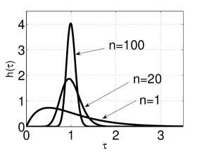
Figure 1: Graphs of $h(\tau)$ at $T=1$ for $n=1,20,100$.

We can exploit the convolution form of (5) and turn it into a differential equation for $r(t)$. Taking a Laplace Transform, we have, for the case of Lorentzian $g(\omega)$,

$$\bar{r}(s)=H(s)\bar{a}^{*}(s),$$ (15)

where $\bar{r}(s)$ and $\bar{a}(s)$ are the Laplace transform of $r(t)$ and $a(t)$ respectively, while

$$H(s)=[(T/\beta_{n})s+1]^{-(n+1)},$$ (16)

is the Laplace transform of $h(\tau)$. Our choice of the function class given by Eq.(12) is motivated by the fact that it yields a particularly convenient Laplace transform and corresponding time-domain formulation. In particular, transforming back to the time-domain by letting $s\rightarrow d/dt$, Eq.(15) yields

$$\left[(T/\beta_{n})(d/dt)+1\right]^{n+1}r(t)=a^{*}(t).$$ (17)

Thus, we now have Eqs.(11) and (17) as our description for the dynamics on the invariant manifold with heterogeneous link delays. Here, it is noteworthy that Eqs.(11) and (17) form a system of ordinary differential equations in comparison with the original system Eq.(1) which comprises a very large number of time-delay differential equations. Note that for the case of uniform delay, $h(\tau)=\delta(\tau-T)$, we take the limit $n\rightarrow\infty$, in which case Eq.(15) takes the form $\bar{r}(s)=e^{-sT}\bar{a}^{*}(s)$, yielding $r(t)=a^{*}(t-T)$, which, when substituted into Eq.(11), gives the time-delay differential equation for $a(t)$ in Ref.OA .

A trivial exact solution to the system (11) and (17) is given by $r(t)=a(t)=0$, which we refer to as the “incoherent state” note1 . Stability of the incoherent state can be studied by linearizing Eq.(11) about the solution $a(t)=0$ and setting $a(t)=a_{0}e^{st}$, from which we obtain

$$1=[kH(s)/2](s+i\omega_{0}+\Delta)^{-1}.$$ (18)

The critical coupling $k_{c}$ at which a stable incoherent state solution becomes unstable as $k$ increases through $k_{c}$, corresponds a solution to Eq.(18) with $\textrm{Re}(s)=0$.

The solid curves in Fig.2 show results obtained from Eq.(18) with Lorentzian $g(\omega)$ for the critical coupling value $k_{c}$ versus $T$ at different $n$’s with parameters $\omega_{0}=3$ and $\Delta=1$. For the case of uniform delays ($n\rightarrow\infty$), $k_{c}$ as a function of $T$ exhibits the type of dependence found in Ref.YS with characteristic “resonances”. However, as the relative spread $\delta\tau/T$ is increased ($n$ is decreased), we see that the resonant structure that applies for the case of zero spread is strongly modified. For example, even at the relatively small spread of $\delta\tau/T\approx 0.1$ (corresponding to $n=100$), there is only one peak (at $T\approx 1$) and one minimum (at $T\approx 2$), with $k_{c}$ for $T>2$ being very substantially higher than in the case of no spread. For $\delta\tau/T\approx 0.302$ ($n=10$) the effect is even more severe, and the previous resonant structure is completely obliterated. For comparison, the dashed curves in Fig.2 show results for $\delta\tau/T\approx 0.302$ (upper) and $0$ (lower) when $g(\omega)$ is Gaussian with the same peak value as for the Lorentzian distribution used to obtain the solid curves note3 . The Gaussian and Lorentzian results are similar, suggesting that the qualitative behavior does not depend strongly on details of $g(\omega)$.

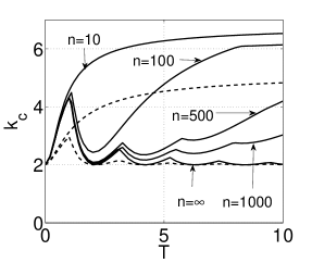
Figure 2: Solid curves are plots of the critical value of $k_{c}$ versus $T$ for Lorentzian $g(\omega)$ with $\omega_{0}=3,\Delta=1$, and $n=10,100,500,1000,\infty$, corresponding to $\delta\tau/T\approx 0.302,0.1,0.045,0.032,0$. The dashed curves are for Gaussian $g(\omega)$ as described in the text.

As reported in Ref.YS , bistable behavior can exist; i.e., a situation in which both incoherent and coherent states are stable. In Figs.3 and 3 we show the hysteresis loops obtained by numerical solution of Eqs.(11) and (17) for $n<\infty$ and, for $n=\infty$, where the $n=\infty$ result is obtained by solution of the delay equation obtained by inserting $r(t)=a^{*}(t-T)$ in (11). Comparing Fig.3, which is for $T=1$, with Fig.3, which is for $T=3$, we note the striking result that, for large $T$, hysteresis is sustained only with large enough spread in the delay distribution, i.e., when $n$ is small [e.g., for $n=\infty$ and $T=3$ (Fig.3) the bifurcation is supercritical and hysteresis is absent].

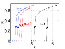
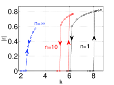
Figure 3: (Color online) Hysteresis loop at $\omega_{0}=3$, $\Delta=1$, (a) for $T=1$, (b) for $T=3$.

Coherent oscillatory states can be obtained by substituting the ansatz $a(t)=a_{0}e^{i\Omega t}$, where $a_{0}$ and $\Omega$ are real constants, into Eq.(10) and (11). This gives

$$\left[i(\Omega+\omega_{0})+\Delta\right]+ (k/2)\left(a_{0}^{2}H^{*}(i\Omega)-H(i\Omega)\right)=0,$$

$$r(t) =a_{0}e^{-i\Omega t}H^{*}(i\Omega).$$ (19)

As reported in both YS and CKK , for $h(\tau)=\delta(\tau-T)$, multiple branches of coherent state solutions are possible in Eq.(19). Furthermore, we can employ Eqs.(11) and (17) to study the stability of each coherent state by introducing a small perturbation $\delta a(t)e^{i\Omega t}$ to the coherent state solution in (19), with $\delta a(t)=K_{1}e^{st}+K_{2}e^{s^{*}t}$. This yields the following equation for $s$:

$$\begin{array}[]{l}[s-\frac{k}{2}H(s+i\Omega)+A][s-\frac{k}{2}H(s-i\Omega)+A^{*}]\\ =\left(ka_{0}^{2}/2\right)^{2}H(s-i\Omega)H(s+i\Omega),\end{array}$$ (20)

where $A=\Delta+i(\omega_{0}+\Omega)+ka_{0}^{2}H(-i\Omega)$. Instability of each coherent state is then determined by whether there are solutions to (20) for $s$ with positive real parts. In Fig.4 we compare the theoretical results for $|r|$ calculated from Eqs.(19) and (20) with simulation results based on Eq.(1) with $N=100$ and $\delta\tau/T\approx 0.1$ ($n=100$) for the first two branches of coherent states with $\omega_{0}=3,\Delta=0.1,T=1$. The solid (dashed) curves correspond to stable (unstable) coherent states. The Eq.(1) simulation values reported in the figures represent time averages of these quantities computed after the solution has apparently settled into the coherent state. It is seen that there is good agreement between the theory and simulations using Eq.(1). In addition, on simulating these two branches of coherent states, we verified that the finding of Ref.CKK that the basin of attraction is large for the first branch, but small for the second one, also holds with heterogeneous delays.

Furthermore, the number of coherent attractors strongly depends on the spread in delay times. Figure 4 shows the dependence of the number of coherent attractors on the relative delay spread $\delta\tau/T=(n+1)^{-1/2}$, with $k=40,\omega_{0}=0,T=1$, for two values of the frequency spread, $\Delta=5$ (dashed) and $\Delta=10$ (solid) (for which $k_{c}=10$ and $20$, respectively). For both cases, it is seen that as the relative delay spread is increased ($(n+1)^{-1/2}$ is increased), the number of coherent attractors decreases. And there remains at least one such attractor when $n$ approaches unity, while a parameter dependent maximum is attained when $n\rightarrow\infty$, which we find is generally larger for smaller $\Delta$ and larger $k$ note2 .

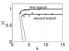
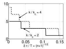
Figure 4: (a) Magnitude of $r$ for the first two branches of coherent states with parameter values: $\omega_{0}=3,\Delta=0.1$, $n=100,T=1$ for $h(\tau)$. Solid lines give the theoretical values of the stable coherent states, dashed lines give the unstable coherent states, and asterisks give the simulation results. (b) Number of coherent attractors (number of solutions of Eq.(19) that are stable according to (20)) versus $\delta\tau/T$ for the following parameters: $k=40,T=1,\omega_{0}=0$; $\Delta=10$ for the solid line ($k_{c}=20$), $\Delta=5$ for the dashed line ($k_{c}=10$).

In conclusion, in this paper we address, for the first time, the effect of heterogeneous delays on the dynamics of globally coupled phase oscillators. As compared to the case of uniform delay (Refs.YS ; CKK ; Park ), we find that delay heterogeneity can have important consequences, among which are the following: (i) decrease in resonant structure of the dependence of $k_{c}$ on $T$ (Fig.2); (ii) increase of $k_{c}$ (Fig.2); (iii) enhancement of hysteretic effects (Figs.3 and 3); (iv) reduction in the number of coherent attractors (Fig.4). Furthermore, we have introduced a framework for the study of delay heterogeneity that can be readily applied to a variety of extensions of the Kuramoto model, such as communities of oscillator populations with different community dependent characteristics Barretto , non-monotonic $g(\omega)$ Martens , and periodic driving Antonsen (see Ref.OA for more examples).

This work was supported by ONR award N00014-07-0734 and by NSF (Physics).

References

- (1) A. Pikovsky, M. Rosenblum and J.Kurths, Synchronization: A Universal Concept in Nonlinear Sciences (Cambridge University Press, 2004).
- (2) J. Buck, Q.Rev.Biol. 63, 265 (1988).
- (3) S.H. Strogatz, D.M. Abrams, A.McRobie, B. Eckhardt and E.Ott, Nature 438, 43 (2005).
- (4) L. Glass and M.C. Mackey, From Clocks to Chaos: The Rhythms of Life (Princeton University Press, NJ, 1988).
- (5) T.D. Frank, A. Daffertshofer, C.E. Peper, P.J. Beek and H. Haken, Physica D 144, 62 (2000).
- (6) J. Garcia-Ojalvo, M.B. Elowitz and S.H. Strogatz, Proc.Natl.Acad.Sci. 101, 10955 (2004).
- (7) S. Yamaguchi, et al., Sci. 302, 255 (Oct. 10, 2003).
- (8) I.Z.Kiss, Y.Zhai and J.L.Hudson, Sci. 296, 1676 (2002).
- (9) M.K.S. Yeung and S.H. Strogatz, Phys.Rev.Lett. 82, 648 (1999).
- (10) M.Y. Choi, H.J. Kim, D. Kim and H. Hong Phys.Rev.E 61, 371 (2000).
- (11) S. Kim, S.H. Park and C.S. Ryu, Phys.Rev.Lett. 79, 2911 (1997); E. Montbrió, D. Pazó and J. Schmidt, Phys.Rev.E 74, 056201 (2006).
- (12) Y. Kuramoto, International Symposium on Mathematical Problems in Theoretical Physics, Lecture Notes in Physics, vol.39, edited by H. Araki (Springer-Verlag, Berlin, 1975); Chemical Oscillations, Waves and Turbulence (Springer, 1984).
- (13) E. Ott and T.M. Antonsen, Chaos 18, 037113 (2008).
- (14) E. Ott and T.M. Antonsen, arXiv:0902.2773 (2009).
- (15) E. Martens, et al., Phys.Rev.E 79 026204 (2009).
- (16) Note that for , Eq.(4) implies that the oscillators do not interact, and run freely at their natural frequencies whose spread leads to a uniform distribution in phase.
- (17) In the Gaussian case the term in Eq.(18) is replaced by , where , , and is the “plasma dispersion function” (see http://farside.ph.utexas.edu/teaching/plasma/lectures /node82.html).
- (18) Kim et al. Park (and reference therein) propose that the presence of many attractors in a Kuramoto-like model with delay (uniform delay in their treatment) can serve as a mechanism for information storage in the nervous system.
- (19) E. Barreto, B. Hunt, E.Ott and P.So, Phys.Rev.E 77, 036107 (2008); E. Montbrió, J. Kurths, and B. Blasius, Phys.Rev.E 70, 056125 (2004).
- (20) T.M. Antonsen, R.T. Faghih, M. Girvan, E. Ott and J. Platig, Chaos 18, 037112 (2008).