On an alternative explanation of anomalous scaling and how well-defined is the concept of inertial range

M. Kholmyansky¹, A. Tsinober^1,2,

¹ Department of Fluid Mechanics and Heat Transfer, Faculty of Engineering, Tel-Aviv University, Tel-Aviv 69978, Israel

² Institute for Mathematical Sciences and Department of Aeronautics, Imperial College, SW7 2PG London, United Kingdom

Abstract. The main point of this communication is that there is a small non-negligible amount of eddies-outliers/very strong events (comprising a significant subset of the tails of the PDF of velocity increments in the nominally-defined inertial range) for which viscosity/dissipation is of utmost importance at whatever high Reynolds number. These events contribute significantly to the values of higher-order structure functions and their anomalous scaling. Thus the anomalous scaling is not an attribute of the conventionally-defined inertial range, and the latter is not a well-defined concept. The claim above is supported by an analysis of high-Reynolds-number flows in which among other things it was possible to evaluate the instantaneous rate of energy dissipation.

There are a variety of models of higher statistics that have meager or nonexistent deductive support from the NS equations but can be made to give good fits to experimental measurements${}^{\ref{ref:gokr}}$. These include ‘explanations’ of what is called anomalous scaling observed experimentally for higher-order structure functions of velocity and temperature increments, such that their scaling exponents $\zeta_{p}=p/3-\mu_{p}<p/3$ are nonlinear concave functions of the order $p$. Starting with refined similarity hypotheses by Kolmogorov${}^{\ref{ref:kolm}}$ and Oboukhov${}^{\ref{ref:obou}}$, numerous phenomenological models have been proposed to describe these deviations considered as the major manifestation of intermittency in the inertial range${}^{\ref{ref:frish}-\ref{ref:ssya}}$. The dominant of these models has been the multi-fractal formalism${}^{\ref{ref:frish}}$, others claimed the Reynolds number dependence as responsible${}^{\ref{ref:lund}-\ref{ref:qian}}$. The common in all these approaches is the basic, widely accepted premise that in the inertial range, the viscosity plays in principle no role${}^{\ref{ref:ruel}}$ so that nonlinear dependence of the algebraic scaling exponents $\zeta_{p}$ on the moment order p is a manifestation of the inertial-range intermittency${}^{\ref{ref:ssya}}$ with the inertial range defined as $\eta\ll r\ll L$ (with $\eta$ being the Kolmogorov and $L$ — some integral scale). Thus the issue is directly related to what is called inertial (sub)range and how inertial it is.

The main point of this communication is that there is a small non-negligible amount of eddies-outliers/very strong events (comprising a significant subset of the tails of the PDF of $\Delta u_{i}(r)$ in the nominally defined inertial range $\eta\ll r\ll L$) for which viscosity/dissipation is of utmost importance at whatever high Reynolds number. In other words, the inertial range is ill-defined in the sense that not all, but almost all statistics of $\Delta u_{i}(r)$ is independent of viscosity. As long as one deals with low-order statistics of $\Delta u_{i}(r)$ (as Kolmogorov did) this is of little (but not always negligible) importance. However, it appears that these events contribute significantly to the higher-order structure functions and thereby a non-negligible contribution to the higher-order structure functions is dominated by viscosity. In other words, the ‘anomalous scaling’ as exhibited by the behavior of higher-order structure functions is to a large extent due to significant contribution of viscosity/dissipation in the inertial range as commonly defined. The higher the order of the structure function, the stronger is the contribution due to viscosity (i.e. from the tails of the PDFs of $\Delta u_{i}(r)$) and the weaker is the ‘inertial’ contribution (i.e. from the core of those PDFs) to the structure function. Thus it seems problematic to speak about inertial-range behavior of higher-order structure functions.

The support for the above view comes from a recent analysis of high-Reynolds-number data in field experiments${}^{\ref{ref:gkk},\ref{ref:kty}}$. The experimental facilities and related matters are described in these papers and references therein. We give here a very brief reminding on these.

The measurement system, developed by the group of Prof. Tsinober, consists of the multi-hot-wire probe connected to the anemometer channels, signal normalization device (sample-and-hold modules and anti-aliasing filters), data acquisition and calibration unit. The probe is built of five similar arrays. Each calibrated array allows to obtain three velocity components “at a point”. The differences between the properly chosen arrays give the tensor of the spacial velocity derivatives (without invoking of Taylor hypothesis), temporal derivatives can be obtained from the differences between the sequential samples.

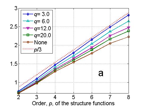
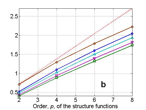
FIG. 1: (a) Scaling exponents of structure functions at $Re_{\lambda}\sim 10^{4}$ for the longitudinal velocity component corresponding to the full data and the same data in which the strong dissipative events (when at least at one point $x$ or $x+r$ the instantaneous dissipation $\epsilon>q\langle\epsilon\rangle$) with various thresholds $q$ were removed. (b) Scaling exponents for the strong events themselves.

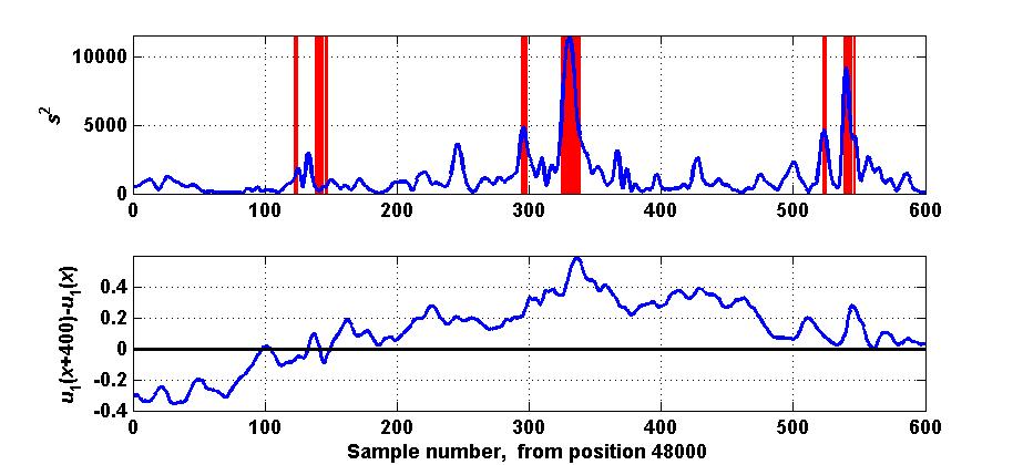
FIG. 2: Example of simultaneous time series of the squared magnitude of the rate of strain tensor, $s^{2}$, proportional to the dissipation $\epsilon$ (top) and the velocity increments, $\Delta u_{1}\equiv u_{1}(x+r)-u_{1}(x)$ for $r=400\eta$ (bottom). The marked segments correspond to the strong events, selected with the value of the threshold $q=12$ equivalent to the value of $s^{2}\approx 4,000$. It should be noted that the first two marked segments are considered strong events because the value of $s^{2}$ reaches the threshold at the point $x+r$.

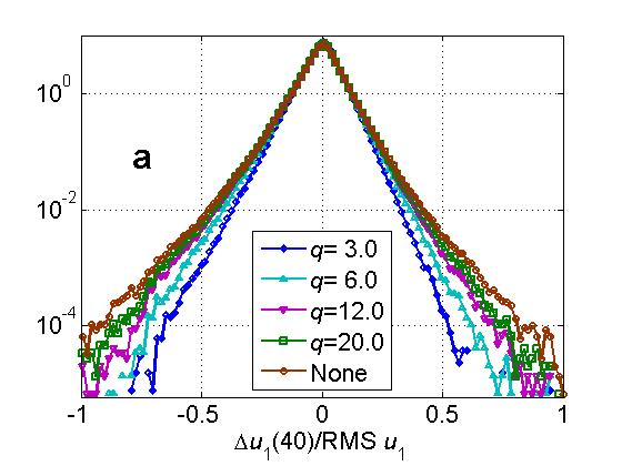
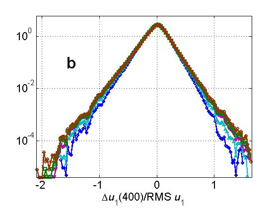
FIG. 3: PDFs of the increments of the longitudinal velocity component for the same data as in Fig. 1. (a) $r/\eta=40$ corresponds to the lower edge of the inertial range. (b) $r/\eta=400$ is deep in the inertial range.

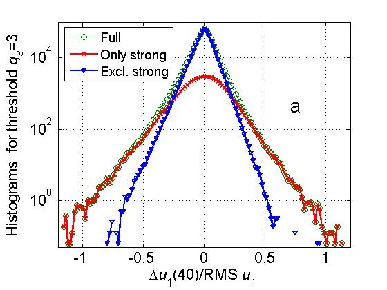
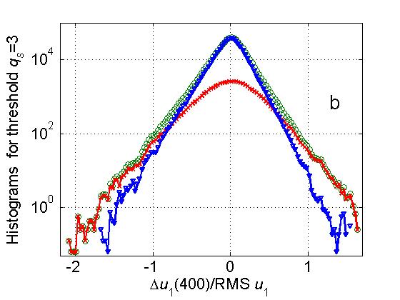
FIG. 4: Histograms of the increments of the longitudinal velocity component for the same data as in Fig. 1 for the threshold $q=3$. $r/\eta=40$ (a). $r/\eta=400$ (b).

The calibration unit produces a jet with variable velocity magnitude and variable angles around two orthogonal axes. The probe is located in the jet core, the values of velocity magnitude and angles are recorded together with the readings of the anemometer channels and later approximated by polynomials, used for obtaining velocity components from the measured hot-wires data.

A selection of results is shown in Fig. 1 — Fig. 6.

Fig. 1 (a) shows the scaling exponents of structure functions $S_{p}^{||}(r)$ up to order 8 corresponding to the full data and the same data in which the strong dissipative events with various thresholds were removed. By an event we mean here a velocity increment, $\Delta u_{1}\equiv u_{1}(x+r)-u_{1}(x)$. It is qualified as a strong dissipative event if at least at one of its ends $(x,x+r)$ the instantaneous dissipation $\epsilon>q\langle\epsilon\rangle$ for $q>1$. We have chosen $q=3,6,12$ and $20$. This corresponds to the instantaneous Kolmogorov-like scales $0.76$, $0.64$, $0.54$ and $0.47$ of the conventional Kolmogorov scale $\eta$ based on the mean dissipation $\langle\epsilon\rangle$. It is seen that the removal of the strong dissipative events results in an increase of the exponents $\zeta_{p}$. For example, with the removal of the dissipative events between the threshold $3\langle\epsilon\rangle$ ($0.76\eta$) and $6\langle\epsilon\rangle$ ($0.64\eta$) the dependence of $\zeta_{p}$ on $p$ becomes pretty close to the Kolmogorov $p/3$. The strong events/outliers themselves have different scaling properties (Fig. 1 (b)). The time series in Fig. 2 illustrate the selection of strong events.

The next example in Fig. 3 shows that indeed the removal of the strong dissipative events results in narrowing of the tails in the PDFs of $\Delta u_{1}(r)$.

As an additional illustration we show in Fig. 4 two examples of histograms of the increments of $u_{1}$ for the whole field, with removed strong dissipative events for the threshold $q=3$ and the dissipative events themselves for the same threshold, for the same data as in Fig. 1.

The effect of the removal of the strong dissipative events is obviously much stronger for higher-order structure functions. For example, there are only $5\%$ of dissipative events (Fig. 5 (a)) for $q=6$ sitting mostly at tails of the PDF of $\Delta u_{i}(r)$ for $r/\eta=400$ (i.e. deep in the ‘inertial’ range), which contribute about $36\%$ to the total dissipation (Fig. 5 (b)). These events contribute nearly $60\%$ to the value of $S_{8}^{\shortparallel}(r)$ at $Re_{\lambda}\sim 10^{4}$ (Fig. 6 (a)). These same events change the $S_{2}^{\shortparallel}(r)$ by about $11.5\%$ (Fig. 6 (b)), but contribute about $9\%$ to $S_{3}^{\shortparallel}(r)$ (see Fig. 6 (c)).

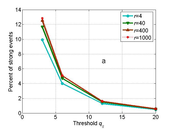
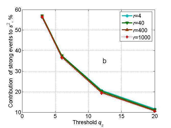
FIG. 5: Percent of the strong dissipative events as defined in the text (a) and their contribution to the total dissipation (b) as a function of the threshold $q$ for various separations $r$.

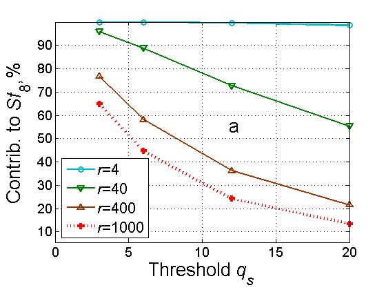
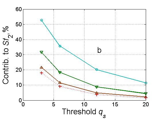
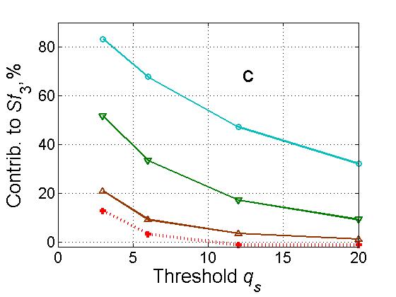
FIG. 6: Contributions of the strong dissipative events, as defined in the text, to the eighth-order structure function (a), the second-order structure function (b) and the third-order structure function (c) as a function of the threshold $q$ for various separations $r$.

It is noteworthy that the data used here${}^{\ref{ref:gkk},\ref{ref:kty}}$ was somewhat spatially underresolved, $1\div 3\eta$. This means that the conclusions are to some extent qualitative. However, with properly resolved data the strong dissipative events, lost in the underresolved ones, would somewhat enhance the tendencies just described above. This is in agreement with the fact that essentially the same results are obtained using the same data smoothed over up to eight sequential samples. Additional support comes from reference${}^{\ref{ref:ssya}}$, indicating that the underresolved data reproduce faithfully the flow at scales about two times smaller than those resolved ($\sim 0.6\eta$) at least as concerns the instantaneous dissipation rate. Finally, using enstrophy $\omega^{2}$ and/or the surrogate $(\partial u_{1}/\partial x_{1})^{2}$ as a criterion for the threshold instead of the true dissipation $\epsilon$ gives the same qualitative (but not quantitative) results.

Summarizing, the main point is the distinction between roughly two kinds of events (in the nominal inertial range $\eta\ll r\ll L$), contributing to the value of the velocity increment. One is represented by the core of the PDF of $\Delta u_{i}$, and the other — by the outliers/extreme events (comprising a significant subset of the tails of the PDF of $\Delta u_{i}$). They have not only different statistical properties (such as scaling if such exists), but also are of different nature in the sense that the former exhibit ‘inertial’ behavior as reflected in the slopes of low-order structure functions, whereas the latter are dominated by viscous effects as seen in the slopes of higher-order structure functions. Removal of these highly-dissipative events brings the dependence of $\zeta_{p}$ on $p$ pretty close to the Kolmogorov $p/3$. Thus the anomalous scaling is not the attribute of the inertial range. Our results leave little doubt that the strong dissipative events contribute significantly to the anomalous scaling of higher-order structure functions. However, there are other effects which are expected to contribute to ‘anomalous scaling’ such as a variety of nonlocal effects understood in a broad sense as direct and bidirectional coupling/interaction between large and small scales${}^{\ref{ref:atsi},\ref{ref:khts}}$. The quality of our data does not allow to address properly this and similar issues. This is a matter of far more precise and well-controlled experiments which among other things require information at high Reynolds numbers with sub-Kolmogorov resolution.

Along with the fact that velocity increments (let alone structure functions and their scaling if such exists) are not the only objects of interest and do not constitute a representation basis for a flow${}^{\ref{ref:gokr}}$, they are not a good object to define a perfect inertial range. Such a definition seems to be not possible in principle due to a variety of nonlocal effects as mentioned above${}^{\ref{ref:atsi},\ref{ref:khts}}$.

A special remark is about the contribution of the dissipative events as defined/described above to the 4/5 law. These events do contribute to the 4/5 law, and removing them leads to an increase of the scaling exponent above unity, see Fig. 1 (a) and Fig. 6 (c). An important point here is that the neglected viscous term in the Karman–Howarth equation does not contain all the viscous contributions. Those which are present in the structure function $S_{3}$ itself remain and keep the 4/5 law precise. It this sense this law is not a pure inertial law. In fact, the contribution of the strongly-dissipative events is non-negligible also in the core of the PDFs of $\Delta u_{1}$ (but not dominating as in their tails) as can be seen from Fig. 4.

Among the main challenges for future work is an experiment similar to that described in references${}^{\ref{ref:gkk},\ref{ref:kty}}$ but with sub-Kolmogorov resolution. This includes also the issue of passive scalar. So far, we have pretty crude qualitative results (due to poor resolution and quality of the data) concerning the passive scalar${}^{\ref{ref:gkk3}}$, which show the same trends as described above and which raise similar questions concerning the anomalous scaling of passive scalars.

• T. Gotoh, and R. H. Kraichnan, “Turbulence and Tsallis statistics,” Physica, D 193, 231–244 (2004).

• A. N. Kolmogorov, “A refinement of previous hypotheses concerning the local structure of turbulence in a viscous incompressible fluid at high Reynolds number,” J. Fluid Mech., 13, 82–85 (1962).

• A. M. Oboukhov, “Some specific features of atmospheric turbulence,” J. Fluid Mech., 13, 77–81 (1962).

• U. Frisch, Turbulence — The Legacy of A. N. Kolmogorov, (Cambridge University Press, 1995).

• A. Tsinober, An informal conceptual introduction to turbulence, (Springer, 2009), in press.

• J. Schumacher, K. R. Sreenivasan, and V. Yakhot, “Asymptotic exponents from low-Reynolds-number flows,” New J. Physics, 9, 89 (1–19) (2007).

• T. S. Lundgren, “Turbulent scaling,” Phys. Fluids, 20, 031301/1–10 (2008).

• V. S. Lvov, and I. Procaccia, “Intermittency in hydrodynamic turbulence as intermediate asymptotics to Kolmogorov scaling,” Phys. Rev. Lett., 74, 2690–2693 (1995).

• T. Nakano, T. Gotoh, and D. Fukayama, “Roles of convection, pressure, and dissipation in three-dimensional turbulence,” Phys. Rev., E67, 026316/1–14 (2003).

• J. Qian, “Normal and anomalous scaling of turbulence,” Phys. Rev., E58, 7325–7329 (1998).

• D. Ruelle, “Conceptual problems of weak and strong turbulence,” Phys. Reports, 103, 81–85 (1984).

• G. Gulitski, M. Kholmyansky, W. Kinzelbach, B. Lüthi, A. Tsinober, and S. Yorish, “Velocity and temperature derivatives in high-Reynolds-number turbulent flows in the atmospheric surface layer. Part 1. Facilities, methods and some general results,” J. Fluid Mech. 589, 57–81 (2007).

• M. Kholmyansky, A. Tsinober, and S. Yorish, “Velocity derivatives in the atmospheric surface layer at $Re_{\lambda}=10^{4}$,” Phys. Fluids 13, 311–314 (2001).

• M. Kholmyansky, and A. Tsinober, “Kolmogorov 4/5 law, nonlocality, and sweeping decorrelation hypothesis,” Phys. Fluids, 20, 041704/1–4 (2008).

• G. Gulitski, M. Kholmyansky, W. Kinzelbach, B. Lüthi, A. Tsinober, and S. Yorish, “Velocity and temperature derivatives in high-Reynolds-number turbulent flows in the atmospheric surface layer. Part 3. Temperature and joint statistics of temperature and velocity derivatives,” J. Fluid Mech. 589, 103–123 (2007).