Spitzer IRAC Detection and Analysis of Shocked Molecular Hydrogen Emission

Abstract

We use statistical equilibrium equations to investigate the IRAC color space of shocked molecular hydrogen. The location of shocked H₂ in $[3.6]-[4.5]$ vs $[4.5]-[5.8]$ color is determined by the gas temperature and density of neutral atomic hydrogen. We find that high excitation H₂ emission falls in a unique location in the color-color diagram and can unambiguously be distinguished from stellar sources. In addition to searching for outflows, we show that the IRAC data can be used to map the thermal structure of the shocked gas. We analyze archival Spitzer data of Herbig-Haro object HH 54 and create a temperature map, which is consistent with spectroscopically determined temperatures.

1. Introduction

Protostellar outflows have strong molecular hydrogen emission in the wavelength range covered by the Spitzer Infrared Array Camera (IRAC). Spitzer studies of known outflows reveal that shocked H₂ emission appears particularly strong in the 4.5 $\mu$m IRAC band (Noriega-Crespo et al., 2004; Teixeira et al., 2008). Many groups are beginning to visually inspect IRAC data to search for outflows and objects with extended H₂ emission based on the strong emission in the 4.5 $\mu$m band. Smith & Rosen (2005) created synthetic Spitzer images from their models of precessing protostellar jets. These models calculated the population of the first three vibrational levels by solving for statistical equilibrium and assuming local thermal equilibrium (LTE) for the rotational levels. Their simulations showed that the emission in the 4.5 $\mu$m band to be the strongest, which was consistent with observations. In taking a census of the young stellar objects (YSOs) in NGC 1333, Gutermuth et al. (2008) empirically determined an IRAC color cut based on observations of known shocked emission within NGC 1333. This was used to remove any possible shocked emission in their source list of YSOs. Due to the multitude of lines in the IRAC bands it was thought that information on the physical parameters of the gas could not be ascertained from the Spitzer IRAC data. In analyzing the IRAC images of IC 443, Neufeld & Yuan (2008) calculated the IRAC band ratios for shocked H₂ using the 13 strongest lines covered by IRAC but only included collisional excitation by H₂ and He in their calculations. They found the measured flux in the 3.6 $\mu$m band to be stronger than predicted in their calculations, which may have been due to neglecting collisional excitation with atomic hydrogen. Until now, the color space of shocked H₂ emission due collisional excitation with atomic hydrogen, He, and H₂ has not been calculated.

In order to use Spitzer IRAC data to find outflows and study their properties we have calculated the IRAC color space of shocked H₂ emission.

2. Calculations

We have calculated the intensities of shocked molecular hydrogen and determined the location of the shocked emission within IRAC color space. At typical shock temperatures and densities, the excitation of molecular hydrogen is through collisions with H atoms and He atoms, and with ground state ortho- and para-H₂ molecules. The typical densities in outflows are less than critical so we do not assume LTE. Instead the populations of the first 47 ro-vibrational excited states were calculated from solving the equations of statistical equilibrium where we set $n(\rm{He})/n_{\rm{H}}=0.10$, $n_{\rm{H}}=n(\rm{H})+2n(\rm{H}_{2})$, and $n(\rm{H})/n(\rm{H}_{2})=0.10$. The atomic hydrogen fraction was set to the median value consistent with shock models and the temperature range we chose (Le Bourlot et al., 2002; Timmermann, 1998). To solve the equations we employed a non-LTE code based on the method by Li et al. (1993). We used the latest H-H₂ non-reactive collisional rate coefficients calculated by Wrathmall et al. (2007). The reactive collisional rate coefficients were derived from the relations of Le Bourlot et al. (1999). The rate coefficients for He-H₂ and H₂-H₂ collisions are from Le Bourlot et al. (1999). The degeneracy of the states is given by $g_{J}=(2J+1)$ for even $J$, and $g_{J}=3(2J+1)$ for odd $J$. The quadrupole transition probabilities used are from Wolniewicz et al. (1998). We calculated the populations of the states over a wide range of atomic hydrogen densities, $n({\rm{H}})=50-10^{5}$ cm^-3, and gas temperatures, $T=1000-6000$ K. The relative intensities of 49 lines that fall within the IRAC bands (3.08 $\mu$m $<\lambda<$ 10.5 $\mu$m) were determined and used to calculate the IRAC band fluxes using the latest published IRAC spectral response (Hora et al., 2008) and calibration data (Reach et al., 2005). Table 1 lists the fractional contribution of the strongest H₂ lines to each IRAC band for $n({\rm{H}})=10^{4}$ cm^-3 and temperatures 2000 K and 4000 K.

Table 1Fractional contribution of the strongest H₂ lines to the IRAC bands

Transition	$\lambda$ ($\mu$m)	IRAC	T=2000 K	T=4000 K
$\nu$ = 1-0 $O$(5)	3.234	1	0.51	0.20
$\nu$ = 2-1 $O$(5)	3.437	1	0.05	0.08
$\nu$ = 1-0 $O$(6)	3.500	1	0.14	0.06
$\nu$ = 2-1 $O$(6)	3.723	1	0.01	0.02
$\nu$ = 0-0 $S$(14)	3.724	1	0.01	0.10
$\nu$ = 1-0 $O$(7)	3.807	1	0.21	0.13
$\nu$ = 0-0 $S$(13)	3.845	1	0.04	0.34
$\nu$ = 0-0 $S$(12)	3.996	2	0.01	0.04
$\nu$ = 0-0 $S$(11)	4.180	2	0.17	0.29
$\nu$ = 0-0 $S$(10)	4.408	2	0.13	0.12
$\nu$ = 1-1 $S$(11)	4.416	2	0.01	0.07
$\nu$ = 0-0 $S$(9)	4.694	2	0.57	0.33
$\nu$ = 1-1 $S$(9)	4.952	2	0.02	0.05
$\nu$ = 0-0 $S$(8)	5.052	3	0.11	0.14
$\nu$ = 0-0 $S$(7)	5.510	3	0.61	0.51
$\nu$ = 1-1 $S$(7)	5.810	3	0.02	0.10
$\nu$ = 0-0 $S$(6)	6.107	3	0.24	0.13
$\nu$ = 0-0 $S$(5)	6.907	4	0.77	0.66
$\nu$ = 1-1 $S$(5)	7.279	4	0.02	0.11
$\nu$ = 0-0 $S$(4)	8.024	4	0.19	0.12

3. H₂ emission in IRAC color space

Figure 1 shows location of shocked H₂ gas in IRAC $[3.6]-[4.5]$ vs. $[4.5]-[5.8]$ color space. We find that the observed emission in the bands is a function of kinetic gas temperature and atomic hydrogen density. We restrict our plot to gas temperatures below 4000 K where H₂ emission is expected to be the dominant. Shocks that would produce gas temperatures in excess of 4000 K are likely to be dissociative (J-type) decreasing the abundance of H₂ molecules. These shocks are also likely to produce vibrationally excited CO emission and fine structure [Fe II] emission in addition to the H₂ emission. The CO molecule, which has a higher dissociation energy than H₂, is able to survive at higher shock velocities and temperatures. In these high energy shocks, CO becomes vibrationally excited and emits in $\nu=1-0$ (4.45 $\mu$m $\lesssim\lambda\lesssim$ 4.9 $\mu$m) lines and can contribute significantly to the total emission from the shocked gas. (González-Alfonso et al., 2002; Draine & Roberge, 1984). Furthermore, the majority of [Fe II] lines in the range covered by IRAC fall within the 4.5 $\mu$m band. Consequently, 4.5 $\mu$m emission in excess to the color space defined by H₂ at 4000 K is likely to trace gas with T $>$ 4000 K placing shocked emission into the upper left portion of the color-color diagram.

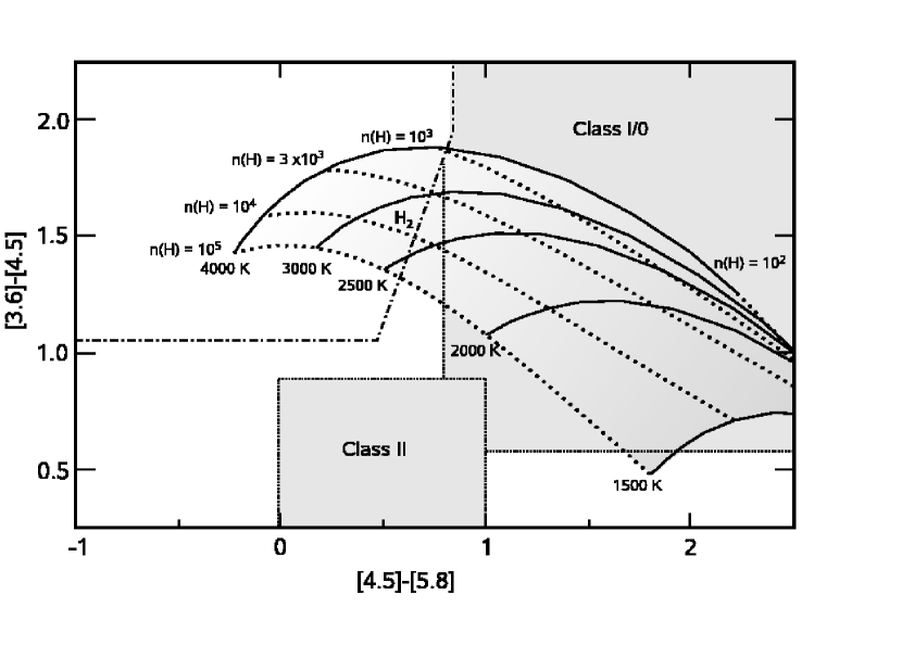
Figure 1.— IRAC $[3.6]-[4.5]$ vs. $[4.5]-[5.8]$ color-color plot indicating the region occupied by shocked H₂. Constant density (dotted) and temperature (solid) lines are indicated. The region to the left and above the dashed-dotted line was empirically determined by Gutermuth et al. (2008) to contain outflows.

We chose not to use the 8 $\mu$m band as there may be dust and PAH contamination in this band. PAH emission is particularly strong in the 8 $\mu$m band and it is still unclear what contribution PAHs may have in the emission of shocked gas from outflows. Dust continuum emission also becomes a possibility as dust may survive the shock. Furthermore our calculations are restricted to a single temperature along the line of sight. In the case of multiple temperature components, the cooler gas will significantly contribute to the lower excitation pure rotational lines, 0$-$0 $S$(4) and 0$-$0 $S$(5), that dominate the emission in the 8 $\mu$m band. The 8 $\mu$m band would then trace the cooler temperature component while the other bands would be more sensitive to the hotter gas. Thus our analysis can include gas containing multiple temperature components along the line of sight but will still be restricted to analyzing only the hotter gas.

As seen in Figure 1, the shocked H₂ lies in a well defined location in the color-color diagram. For comparison, the location of YSOs is also shown in the figure based on the criteria of Gutermuth et al. (2008) and Megeath et al. (2004). Shocked H₂ gas with sufficiently high temperature and atomic hydrogen density is found in a unique location on this diagram and can be distinguished from YSOs. This is consistent with the empirically determined color cut of Gutermuth et al. (2008). Therefore these colors offer an unambiguous method for searching for shocked gas from outflows/jets. However, there is overlap in IRAC color space between low temperature shocked H₂ gas and protostellar sources. Consequently surveys searching for outflows using IRAC color analysis will be restricted to finding flows containing higher excitation gas. Additional data at different wavelengths (2MASS, MIPS, etc.) and/or morphology may be able to break this degeneracy. Our results are consistent with empirical observations of strong 4.5 $\mu$m emission in outflows and with the hydrodynamic simulations of Smith & Rosen (2005).

Using this color analysis, two methods can be applied to identify outflows in the images: 1) Visual inspection of 3-color images constructed out of the 3.6 $\mu$m, 4.5 $\mu$m, and 5.8 $\mu$m band data with appropriate scaling to enhance the shocked emission, and 2) analysis of the photometry of the field where features consistent with colors of shocked H₂ emission are selected. This can be accomplished by evaluating the color pixel by pixel across the field.

The location of the shocked H₂ in color space depends on its temperature. Therefore color analysis provides a new way to probe the temperature structure of the gas. This can be accomplished by evaluating the colors pixel by pixel across the field. The colors can then be compared to the colors of shocked H₂ and the temperature of the gas can be estimated. Resulting temperature maps are restricted to temperatures between $2000-4000$ K and high atomic hydrogen densities. The color space for H₂ at temperature less than 2000 K moves further into the color space of Class I/0 objects and it becomes more likely to misidentify scattered light from YSOs as H₂ emission. Note that, at low atomic hydrogen densities the constant temperature lines start to converge and thus temperature estimates from this region of color space may have large uncertainties.

4. Example

We applied our analysis to Spitzer archival data of the known outflow HH 54 (catalog ). We evaluated the IRAC colors at each pixel in the field of HH 54. The median value of the image was used to estimate the background and was subtracted from the images. Figure 2 shows the color-color diagram for the knots (A,B,C,E,K,M) of shocked H₂ previously studied by Giannini et al. (2006). We plot all the pixels on the diagram that are encompassed by the knots. The majority of points fall within our calculated color space for shocked H₂ emission. One exception is knot A which contains several pixels with colors that fall more than 3$\sigma$ outside the 4000 K boundary. This region of color space with excess 4.5 $\mu$m emission is consistent with higher gas temperatures and possible additional emission from CO $\nu=1-0$ and [Fe II].

Giannini et al. (2006) obtained spectroscopic data of various knots in HH 54 in the near-infrared and used H₂ emission lines to estimate the rotational and vibrational excitational temperatures of the gas. We created a temperature map of HH 54 (figure 3) by selecting the pixels whose colors fall within the range we identified as belonging to shocked H₂ ($T=2000-4000$ K) and $[4.5]-[5.8]\leq 1.5$, and then estimated the temperature of the gas based on the pixels location in color space. The estimated temperatures are compared to the vibrational ($\nu\geq 1$) excitation temperatures obtained by Giannini et al. (2006) in table 2. Because typical atomic hydrogen densities in shocks are less than critical, the gas cannot be assumed to be in LTE. In these environments the rotational temperatures are often far below the kinetic gas temperature, while the ro-vibrational $\nu\geq 1$ excitation temperatures are close to the kinetic gas temperature. For most of the knots the temperatures we estimate from color analysis and the spectroscopically determined temperatures are consistent.

There is an additional knot, labeled I ($\alpha_{\rm{J2000}}$=12:55:54.8, $\delta_{\rm{J2000}}$=-76:56:06), 5 arcseconds to the east of knot C seen in the IRAC images that is not found in the NIR images of HH 54 which we identify as the mid-infrared counterpart to the optical knot HH 54I (catalog ) (Sandell et al., 1987). The temperature of the gas in this knot peaks at 3500 K as seen in figure 2 and 3. This knot is also found on the edge of the [Ne II] 12.8 $\mu$m map of HH 54 by Neufeld et al. (2006). The presence of the fine-structure [Ne II] line is consistent with the high temperature structure of this knot. Knot B ($T\sim 2600$ K)is also found to be spatially coincident with strong [Ne II] 12.8 $\mu$m emission. The distribution of the [Fe II] 26 $\mu$m line (Neufeld et al., 2006) covers a region containing knots A, B, M. We find that spatial distribution of fine-structure emission lines is consistent with regions within our temperature map where $T\gtrsim 2600$ K. Knots A, B, and I are spatially aligned with each other as indicated by the green line in figure 3. These high temperature knots may trace the jet component of the outflow. This line points in the direction of IRAS 12496-7650 which is believed to be the source of the outflow.

Table 2Temperature estimates of HH 54

Knot	$\alpha$(J2000)	$\delta$(J2000)	$T_{gas}$	$T_{\nu\geq 1}$
A	12:55:49.5	-76:56:30	3300$\pm$500 K	3000$\pm$150 K
B	12:55:51.1	-76:56:21	2600$\pm$300 K	3000$\pm$140 K
C	12:55:53.1	-76:56:06	2200$\pm$100 K	2960$\pm$150 K
E	12:55:53.8	-76:56:23	2000$\pm$100 K	2500$\pm$90 K
K	12:55:54.3	-76:56:25	2100$\pm$100 K	2500$\pm$90 K
M	12:55:51.6	-76:56:13	2800$\pm$400 K	3000$\pm$140 K

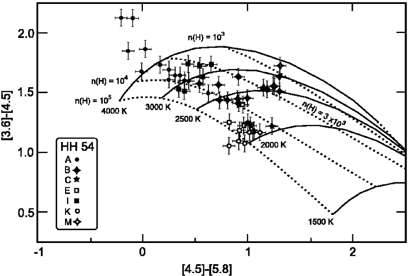
Figure 2.— IRAC color-color plot for identified knots in HH 54. Each point represents the colors at an individual pixel within the knots. Different knots are represented with different symbols.

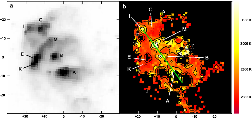
Figure 3.— a) IRAC 4.5$\mu$m image of HH 54. Image center is at $\alpha$(J2000) = 12^h55^m49$\fs$5 $\delta$(J2000) = -76°56′22″. Individual knots are identified and labeled according to Giannini et al. (2006). Knot I, not seen on the NIR, is identified as the optical counterpart to HH 54I b) Temperature map of HH 54 based on IRAC color-color analysis for 2000 K $\leq T\leq$ 4000 K. The black contour levels are 2000 K, 2500 K, 3000 K, and 3500 K. The green line connecting the higher temperature knots A, B, and I points toward the proposed source IRAS 12496-7650.

5. Conclusions

We have quantitatively shown that analysis of Spitzer data can be used to discover and characterize emission from protostellar outflows. Shocked H₂ with sufficiently high temperature and neutral atomic hydrogen density can be distinguished unambiguously from stellar objects in IRAC color space. IRAC color analysis is useful for studying intermediate-excitation shocked gas within the temperature range $T=2000-4000$ K. Higher temperature gas may contain significant contribution from ionic lines like [Fe II] and also from the CO $\nu=1-0$ emission band. Even with this limitation, Spitzer IRAC data provides a useful tool in the study of outflows. In particular, IRAC color analysis can be used to probe the thermal structure of the gas without the need of using spectroscopic data.

References

- Draine & Roberge (1984) Draine, B. T., & Roberge, W. G. 1984, ApJ, 282, 491
- Giannini et al. (2006) Giannini, T., McCoey, C., Nisini, B., Cabrit, S., Caratti o Garatti, A., Calzoletti, L., & Flower, D. R. 2006, A&A, 459, 821
- González-Alfonso et al. (2002) González-Alfonso, E., Wright, C. M., Cernicharo, J., Rosenthal, D., Boonman, A. M. S., & van Dishoeck, E. F. 2002, A&A, 386, 1074
- Gutermuth et al. (2008) Gutermuth, R. A., et al. 2008, ApJ, 674, 336
- Hora et al. (2008) Hora, J. L., et al. 2008, PASP, 120, 1233
- Irwin (1987) Irwin, A. W. 1987, A&A, 182, 348
- Le Bourlot et al. (1999) Le Bourlot, J., Pineau des Forêts, G., & Flower, D. R. 1999, MNRAS, 305, 802
- Le Bourlot et al. (2002) Le Bourlot, J., Pineau des Forêts, G., Flower, D. R., & Cabrit, S. 2002, MNRAS, 332, 985
- Li et al. (1993) Li, H., McCray, R., & Sunyaev, R. A. 1993, ApJ, 419, 824
- Megeath et al. (2004) Megeath, S. T., et al. 2004, ApJ, 154, 367
- Neufeld et al. (2006) Neufeld, D. A., et al. 2006, ApJ, 649, 816
- Neufeld & Yuan (2008) Neufeld, D. A., & Yuan, Y. 2008, ApJ, 678, 974
- Noriega-Crespo et al. (2004) Noriega-Crespo, A., et al. 2004, ApJS, 154, 352
- Reach et al. (2005) Reach, W. T., et al. 2005, PASP, 117, 978
- Sandell et al. (1987) Sandell, G., Zealey, W. J., Williams, P. M., Taylor, K. N. R., & Storey, J. V. 1987, A&A, 182, 237
- Smith & Rosen (2005) Smith, M. D., & Rosen, A. 2005, MNRAS, 357, 1370
- Teixeira et al. (2008) Teixeira, P. S., McCoey, C., Fich, M., & Lada, C. J. 2008, MNRAS, 384, 71
- Timmermann (1998) Timmermann, R. 1998, ApJ, 498, 246
- Waech & Bernstein (1967) Waech, T. G., & Bernstein, R. B. 1967, J. Chem. Phys., 46, 4905
- Wolniewicz et al. (1998) Wolniewicz, L., Simbotin, I., & Dalgarno, A. 1998, ApJS, 115, 293
- Wrathmall et al. (2007) Wrathmall, S. A., Gusdorf, A., & Flower, D. R. 2007, MNRAS, 382, 133