Pulsars versus Dark Matter
Interpretation of ATIC/PAMELA
Abstract
In this paper, we study the flux of electrons and positrons injected by pulsars and by annihilating or decaying dark matter in the context of recent ATIC, PAMELA, Fermi, and HESS data. We review the flux from a single pulsar and derive the flux from a distribution of pulsars. We point out that the particle acceleration in the pulsar magnetosphere is insufficient to explain the observed excess of electrons and positrons with energy TeV and one has to take into account an additional acceleration of electrons at the termination shock between the pulsar and its wind nebula. We show that at energies less than a few hundred GeV, the flux from a continuous distribution of pulsars provides a good approximation to the expected flux from pulsars in the Australia Telescope National Facility (ATNF) catalog. At higher energies, we demonstrate that the electron/positron flux measured at the Earth will be dominated by a few young nearby pulsars, and therefore the spectrum would contain bumplike features. We argue that the presence of such features at high energies would strongly suggest a pulsar origin of the anomalous contribution to electron and positron fluxes. The absence of features either points to a dark matter origin or constrains pulsar models in such a way that the fluctuations are suppressed. Also we derive that the features can be partially smeared due to spatial variation of the energy losses during propagation.
pacs:
97.60.Gb, 95.35.+d, 96.50.S-, 98.70.SaI Introduction
The nature of dark matter (DM) remains one of the most interesting problems in cosmology and astrophysics. Recently, several cosmic ray experiments reported higher than expected fluxes of electrons and positrons at energies between 10 GeV and 1 TeV :2008zzr ; Adriani:2008zr ; Collaboration:2008aaa ; Aharonian:2009ah ; Abdo:2009zk . One interpretation is that this excess is a result of DM annihilation or decay Cholis:2008vb ; Bergstrom:2008gr ; Cirelli:2008pk ; Cholis:2008hb ; ArkaniHamed:2008qn ; Yin:2008bs ; Hamaguchi:2008rv ; Chen:2008fx . Standard astrophysical sources, such as pulsars 1995A&A…294L..41A ; Kobayashi:2003kp ; Hooper:2008kg ; Yuksel:2008rf ; Profumo:2008ms ; Ioka:2008cv , are also a viable possibility. The main purpose of this work is to identify an observational signature which might differentiate between these two models.
Pulsars are known to produce and accelerate electrons and positrons in their magnetosphere Rees:1974nr . However, as we will argue below, this acceleration is insufficient to explain the observed excess. Moreover, the spectrum of particles in the magnetosphere is further modified at the termination shock between the pulsar and the interstellar medium (ISM) or the supernova remnant (SNR) which may contain the pulsar wind nebula (PWN). It is important to emphasize that termination shocks are observed around middle-aged pulsars (e.g., Geminga 2003Sci…301.1345C ; Pavlov:2005wc , PSR J1747-2958 Gaensler:2003iy ) and not just young pulsars like the Crab. Most young energetic pulsars are also surrounded by a PWN (for a review see, e.g., Gaensler:2006ua ) which is powered by the continuous emission from the pulsar and remains inside the shell or envelope produced by the initial explosion (a discussion of various regions surrounding a pulsar can be found in, e.g., Kennel:1984vf ). Inside a PWN, the electrons and positrons are confined by the nebula’s magnetic field for a long period of time before escaping into the ISM. Since a pulsar loses the vast majority of the spin-down energy while its PWN still exists, we assume that most of the electrons and positrons injected by pulsars spend a significant amount of time inside a PWN before reaching the ISM. This has two main consequences:
-
•
The spectrum of electrons and positrons injected by a pulsar into the surrounding ISM is not the spectrum of particles inside the magnetosphere (as assumed by many authors, e.g Hall:2008qu ; Hooper:2008kg ; Profumo:2008ms ), but the spectrum of particles that escape the PWN into the surrounding ISM. In this paper, we assume that this is the same as the electron/positron spectrum inside the PWN when it is disrupted, which we estimate using the observed broadband spectrum of these objects.
-
•
Since the lifetime of a PWN ( kyr; Gaensler:2006ua ) is generally much smaller than the typical propagation time ( kyr), the electrons observed at the Earth come from PWNe that no longer exist, whereas electrons inside existing PWNe cannot reach us. Since the variability of PWNe properties is very large, we cannot predict the electron flux from a pulsar that has already lost its PWN, even if we fully know its current properties (e.g age, position, spin-down luminosity).
Therefore, the best one can do is to use the currently observed PWNe to derive a statistical distribution of their properties. This distribution can be used to find either the average flux of electrons expected from pulsars or, by assigning the PWNe random properties according to the distribution, the typical electron flux observed on Earth from all pulsars.
The observed spectrum on Earth of electrons and positrons injected by pulsars is also strongly dependent on propagation effects. In particular, the observed cutoff in the flux of electrons from a pulsar can be much smaller than the injection cutoff due to energy losses (“cooling”) during propagation. We define the cooling break, , as the maximal energy electrons can have after propagating for time . Since – as stated above – the typical electron propagation time is much larger than the lifetime of a PWN, we can assume that a pulsar is a delta-function source and the propagation time for electrons from this pulsar can be estimated by the pulsar’s age . If the cooling break is at a lower energy than the injection cutoff from a PWN, , then the observed break is the cooling break which depends on the age of the pulsar but is independent of the injection cutoff. Since the cooling break is much steeper than the injection break, the existence of several pulsars with sufficiently close to the Earth such that the propagation time of electrons they inject into the ISM is less than their age will result in a sequence of steps or bumps in the spectrum. At high energies, only a few pulsars will satisfy this criterion, so these steps are expected to be well separated and therefore observable. At lower energies, we expect many pulsars to contribute, causing these steps to be averaged together and resulting in a smooth spectrum. We argue that the presence of significant steps, or bumps, in the electron spectrum at high energies would strongly suggest this excess is generated by pulsars, since the flux from the dark matter is expected to be smooth with a single cutoff. If these features are not observed, a pulsar explanation of the observed excess is possible if there are no young energetic pulsars in the vicinity of the Earth with Grasso:2009ma or there are considerable spatial variations in the energy losses of these particles as they diffuse through the ISM. The amplitude of these fluctuations also depends on the relative contributions of the backgrounds and the pulsars. If backgrounds dominate at high energies, these fluctuations may be undetectable.
This paper is organized as follows: In Sec. II, we review the propagation of electrons in the ISM. We estimate the typical propagation time and distance for electrons and positrons of a given energy and show that injection of electrons and positrons by a pulsar can be approximated by delta-functions in space and time. Using the properties of pulsars and their PWN derived in Appendix A, we derive the temporal evolution of the observed flux from a single pulsar at a given distance. In Sec. III, we study the flux from a distribution of pulsars, calculating the average expected flux and comparing this result to the estimate flux from pulsars in the Australia Telescope National Facility (ATNF) catalog Manchester:2004bp – demonstrating that at energies GeV this flux is well approximated by the average curve while at higher energies there are significant deviations and bumplike features due to the cooling breaks. We then compare both spectra with the ATIC, Fermi-LAT, and PAMELA data. In Sec. IV, we review the flux from dark matter. In Sec. V, we present our conclusions. We argue that the flux from dark matter is likely indistinguishable from the flux from a single pulsar or from a continuous distribution of pulsars. Thus, unless there are additional features at high energies that point to the contribution from several pulsars, it may be impossible to tell whether the excess is due to dark matter or pulsars.
The paper also contains a few appendixes: In Appendix A we give a general review of pulsars and pulsar wind nebulae. In Appendix B we derive the smearing of the cooling breaks due to spatial variability of energy losses. In Appendix C we study some constraints that current electron and positron data put on the pulsar models.
II Single pulsar flux
The flux of cosmic ray electrons at the Earth depends on both the spectrum of injected electrons and the properties of the ISM. First, we review the propagation of electrons in the ISM, and then derive the expected flux from pulsars and dark matter.
II.1 Properties of the interstellar medium
The ISM contains a magnetic field with a strength on the order of Longair1992 . Since the corresponding Larmor radius for a 1 TeV electron is small, pc, electrons are expected to mostly follow the ISM’s magnetic field lines. Because the ISM magnetic field has random fluctuations, electrons propagate along on a random path. The corresponding diffusion coefficient for relativistic particles is Strong:2007nh
| (1) |
where and for GeV. [The typical mean free path for a 1 TeV electron pc is much larger than the Larmor radius pc.] We find it convenient to express the diffusion coefficient in terms of the energy rather than the magnetic rigidity, , where is the momentum and is the charge of the particle. In our case, the two definitions are equivalent.
As electrons propagate in the ISM, they lose energy. For electrons with energy GeV, the dominant loss mechanisms are synchrotron radiation and inverse Compton scattering off cosmic microwave background, infrared (IR), and starlight photons. The corresponding energy losses are
| (2) |
where for the local density of photons Porter:2005qx and . Before we present a formal solution to the propagation equations, we define a few characteristic numbers. In estimations, it is convenient to represent the parameters in the units of pc cm and kyr = s. In this paper we will usually use and with .
By integrating Eq. (2), we find the energy loss in terms of the electron travel time is
| (3) |
where is the initial energy of the electron and is the energy at time . The cooling break, defined as the maximal energy an electron can have after traveling for time , is
| (4) |
The characteristic travel time is therefore
| (5) |
The characteristic distance an electron travels before cooling to energy is the diffusion distance , where ,
| (6) |
II.2 Green function for diffusion-loss propagation
In general, the evolution of the energy density of electrons moving in random paths and losing energy can be described by the following diffusion-loss equation Longair1992 Ginzburg1964
| (7) |
where is the energy density of electrons injected by the source. In principle, one can also take into account reacceleration, convection, and decays (collisions), but for electrons with GeV these contributions can be ignored.
The general solution to Eq. (7) is found in Ginzburg1964 1959AZh….36…17S . To solve Eq. (7) for a general source, one introduces the Green function which satisfies
| (8) |
Then, the solution to (7) is
| (9) |
The Green function can be derived as follows. One can define the variables and Ginzburg1964 1959AZh….36…17S , where
| (10) | |||
| (11) |
The variable is invariant with respect to the differential operator . In fact, and Eq. (8) becomes the usual diffusion equation in and . The Green function is then Ginzburg1964 1959AZh….36…17S
| (12) |
Equation (7) and the above Green function have a few limitations. Both the ISM magnetic field and density of IR and starlight photons vary in space. Consequently the diffusion coefficient and the energy loss function depend on the coordinates: , , and there is no simple analytic solution to Eq. (7). In Appendix B we calculate corrections to the predicted spectrum at the Earth due to spatial variations in the energy loss function.
II.3 Flux from a single pulsar
With the general Green function in hand, one can find the density of electrons at any point in space for any source. In this Section, we derive the expected flux of electrons and positrons produced by a single pulsar.
The distances to pulsars are sufficiently large that we can assume that pulsars are point sources. We also assume that most of the pulsars’ rotational energy is lost via magnetic dipole radiation Shapiro1983 which eventually transforms into the energy of electrons and positrons
| (13) |
where is the pulsar age and is its position. is the step function that ensures for . Note that the pulsar spin-down time scale in this formula and the variable introduced in (10) are unrelated. We review the derivation of this formula in Appendix A.
At late times (), the spin-down luminosity scales as . Consequently, most of the energy is emitted during . The pulsar spin-down time scale kyr is much smaller than the typical electron propagation time kyr. Consequently, we can take the limit , which results in
| (14) |
For pulsars with a significant PWN, the time dependence in Eq. (13) does not describe the escape of electron and positrons from the PWN into the ISM. However, for most pulsars the lifetime of the PWN ( kyr; Gaensler:2006ua ) is much smaller than the typical propagation time kyr [Eq. (5)]. Thus, the detailed time dependence of the escape is not significant and the delta-function approximation in Eq. (14) is still valid.
We assume that the energy spectrum of particles injected into the ISM by a given pulsar has the form
| (15) |
where is the injection index and is the injection cutoff. We denote the initial rotational energy of the pulsar by and define to be the fraction of this energy deposited in the ISM as . The total energy emitted in is then
| (16) |
For , this gives
| (17) |
The index and the cutoff of the electron spectrum can be derived from the broadband spectrum of a PWN, and may vary significantly between pulsars. We argue in Appendix A that reasonable values for energetic pulsars are and .
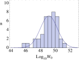
The overall normalization is more difficult to derive because neither the initial rotational energy nor the conversion efficiency are known for most pulsars. Currently, models can only estimate to an order of magnitude with significant theoretical uncertainties FaucherGiguere:2005ny . In Appendix A, we derive that, assuming a constant pulsar time scale kyr for all pulsars in the ATNF catalog Manchester:2004bp , the distribution of pulsar initial rotational energies erg satisfies a log-normal distribution with and which gives the average erg. If we use kyr, the same analysis gives , , and erg. If the age of a pulsar is known independently, then the initial rotational energy can be estimated more robustly. For example, the Crab pulsar is associated with the SN1054 supernova explosion and has kyr and erg.
Let us now discuss the conversion coefficient . The energy density near the surface of the pulsar is dominated by the magnetic field and the spin-down luminosity is dominated by the magnetic dipole radiation. In most PWNe the energy density is believed to be particle dominated, i.e. at large distances from the neutron star most of the energy outflow has been converted to particles and at this stage (see, e.g., 1996MNRAS.278..525A for a discussion of the Crab PWN). However, these particles do not immediately escape to the ISM but are trapped inside the PWN by its magnetic field where they can lose a significant fraction of their energy. In Appendix A, we estimate due to cooling of the particles before they escape into the ISM. Based on the discussion above, we find that the average energy in electrons and positrons erg is reasonable. This value is model dependent and can vary greatly from one pulsar to another.
The density of electrons propagated from a pulsar to the Earth can be found by substituting the source function into Eq. (9)
| (18) |
where parameter is defined in Eq. (11) and is the initial energy of the electrons that cool down to in time
| (19) |
The density in Eq. (18) has a cutoff at the cooling break, , since for .
For a density of relativistic particles, the flux is defined as
| (20) |
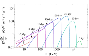
The time evolution of the flux from a single pulsar is shown in Fig. 1. At early times, the electrons have not had enough time to diffuse to the observer and the flux is exponentially suppressed. At later times, the flux grows until the diffusion distance is similar to the distance from the pulsar to the Earth. After that the flux decreases as the electrons diffuse over a larger volume. The cutoff moves to lower energies due to cooling of electrons.
For energies much smaller than the cooling break, we can neglect energy losses. In this case, , and Eq. (18) reduces to
| (21) |
Assuming that , the flux for is
| (22) |
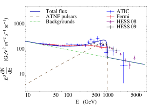
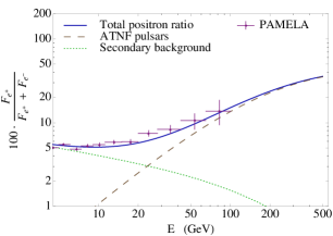
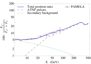
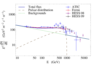
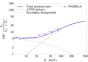
In general, the flux that we add to the backgrounds to fit the data can be effectively parametrized by three numbers: the normalization, the index at low energies, and the cutoff energy. From the right hand side of Eqs. (17) and (22) we find that these three parameters correspond to at least 8 parameters describing the pulsar and the ISM. In particular, the propagated index is a linear combination of and , , the propagated cutoff is , and the normalization depends on , , , , and . In order to fix this degeneracy, as a matter of convenience, we choose , , , erg, and TeV. With this choice, our fit to the data will determine , , and . If some of the parameters are known independently, e.g., the propagation model, the energy losses, the age of the pulsar etc., this approach becomes more constrained and more predictive. As shown in Fig. 2, the expected flux from a pulsar with erg, , distance 0.3 kpc, and age 200 kyr reproduces the positron fraction measured by PAMELA and is a good fit to the cosmic-ray electron spectrum measured by ATIC, Fermi, and HESS below TeV. This suggests that the anomaly in the flux could be due to a single pulsar. However, given the considerable number of known nearby, energetic pulsars Manchester:2004bp , it is unlikely that the flux from any single pulsar is significantly larger than the flux from all such pulsars. In the next section, we will derive the expected flux of electrons and positrons from a collection of pulsars.
III Flux from a collection of pulsars
In this section, we derive the flux from a continuous distribution of pulsars and compare it with the predicted flux from the pulsars in the ATNF catalog Manchester:2004bp .
III.1 Flux derivation
We assume that pulsars are homogeneously distributed in the galactic plane and are born at a constant rate FaucherGiguere:2005ny . The “continuous” distribution of pulsars is defined as the average of all possible realizations of pulsar distributions. This results in a source function constant in time, localized in the vertical direction, and homogeneous in the galactic plane
| (23) |
with the normalization constant
| (24) |
where is the area of the galactic plane. Since the diffusion distance of these electrons is significantly smaller than the distance from the Earth to the edge of the galactic plane FaucherGiguere:2005ny ( kpc), we can neglect the effects of having an edge at a finite distance.

Using the general Green function in Eq. (II.2), the flux of electrons from this distribution is
| (25) |
Integrating over and , we obtain
| (26) |
where is defined in Eq. (11). This flux can be rewritten as
| (27) |
where
| (28) |
for example, if , , and , then .
As in the case of a single pulsar flux, the number of parameters we need to fit the data is much smaller than the number of parameters characterizing the flux from a collection of pulsars. In this case, the index of the observed flux and the normalization can be found from Eq. (27). For example, the index of the flux at low energies . Formally, the cutoff in this case is equal to the injection cutoff , but for an actual distribution of pulsars the expected cutoff is lower and is determined by the age of the youngest pulsar within the diffusion distance from the observer – as derived in Sec. III.2. If we break the degeneracy by picking a particular propagation model, we can constrain the properties of the pulsar distribution. The opposite is also true: by choosing some properties of the pulsars one can constrain the properties of the ISM – as demonstrated in Appendix C.
In order to break the degeneracy we fix the ISM properties as in Sec. II.3. To calculate the flux from the pulsars in the ATNF catalog we use the following toy model. We assume that every pulsar has injection index and conversion efficiency (these values are chosen to fit the low energy electron and positron data in Fig. 4). We choose an injection cutoff TeV for every pulsar (for smaller values of the features at high energies will be less sharp, since the injection cutoff is not as abrupt as the cooling break). In order to estimate the initial rotational energy, we assume that for each pulsar, the spin-down time scale is = 1 kyr. Then we use Eq. (44) to express the initial rotational energy in terms of the current spin-down luminosity and the pulsar age :
| (29) |
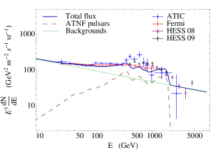
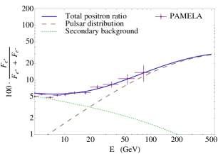
The result in shown in Fig. 3, and the relative normalization between this spectrum and that of the continuous distribution described above depends on the pulsar birth rate , or, to be more precise, on the local value of the pulsar birth rate. In order to have a good agreement between the two curves for energies 30 – 300 GeV, we require , assuming a Milky Way radius = 20 kpc FaucherGiguere:2005ny . For energies below 30 GeV, we find that the main contribution to flux comes from the pulsars with age Myr. These pulsars typically have a very low spin-down luminosity and therefore are difficult to observe (in the ATNF catalog there are very few pulsars with the spin-down luminosities erg). In Fig. 4, we apply to this spectrum the Gaussian smearing expected to result from spatial variations in energy losses depending on the path of the electrons – as derived in Appendix B. As one can see, this provides a very good fit to the PAMELA, Fermi, and HESS data - but does not reproduce the ATIC bump.
Determining the flux of from the actual distribution of pulsars using a more realistic model is extremely difficult because every pulsar has its own independent parameters (e.g., , , and ). Thus, we may choose several thousands of parameters in order to fit less than a hundred of data points (which can be fitted by a flux parametrized by three parameters only). Moreover, as we discussed in the Introduction, these thousands of parameters refer to PWNe sufficiently old that their electrons have had enough time to diffuse to the Earth. These PWNe have already disappeared and therefore cannot be observed directly – making it impossible to directly constrain these parameters observationally. The large number of pulsars and the impossibility to derive their individual properties suggest a statistical method is needed to study the flux they produce. At small energies, a lot of pulsars contribute to the observed flux on Earth and therefore the properties of an individual pulsar are unimportant. In this case, the flux should be well approximated by some average curve – as demonstrated in Fig. 3. In this estimate we included all pulsars with ages kyr and use the delta-function approximation of source functions, (Sec. II). The choice of the lower cutoff on the age of the pulsars is motivated by the fact that young pulsars, such as the Vela pulsar, usually have a PWN and therefore their electrons have not escaped yet into the ISM. At high energies only a few young pulsars contribute and the deviation from the average curve may be large. The presence of features at high energies may serve as a signature of a collection of pulsars that can distinguish them from a dark matter or single pulsar origin for these electrons.
III.2 Statistical cutoff
As shown in Fig. 3, the expected flux from a continuous distribution of pulsar increases with energy until a break at TeV, whereas the predicted flux from pulsars in the ATNF database has a cutoff at 2 TeV. This discrepancy is due to the rare events when a young pulsar is very close to the observer. Since electrons lose energy during propagation, high energy electrons must come from young pulsars and the cutoff energy is determined by the age of the youngest pulsar sufficiently close to the observer so that the electrons have enough time to diffuse through the ISM. We will call the average such cutoff a “statistical” cutoff.
To estimate the statistical cutoff, we consider a collection of pulsars and choose an observation point. The statistical cutoff at this point is the maximal cooling break energy for the flux from these pulsars. In this distribution, the youngest pulsar whose electrons can reach the observation point has an age and diffusion distance . For a given pulsar birth rate , we estimate by demanding that there is at least one pulsar within younger than . Therefore, we have a system of three equations for the three unknowns , and :
| (30) | |||
| (31) | |||
| (32) |
Solving this system of equations, we find
| (33) |
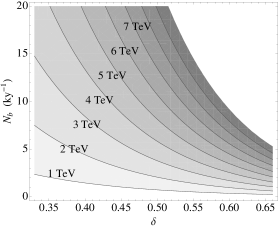
Assuming kpc, , and , we get
| (34) |
where is in units of . In Fig. 5, we show the statistical cutoff as a function of and the diffusion index . This calculation should be viewed as a rough estimate, with the actual flux from the distribution of real pulsars having a cutoff that differs by as much as an order of magnitude. Additionally, it is possible that current data are missing a feature at high energies ( TeV) due to poor statistics. A comparison between the flux from a continuous distribution of pulsars with TeV and the current data is shown in Fig. 6.
We note that Eq. (33) can also be used to find the cutoff in the primary background if we assume that it is generated by the supernova explosions. For instance, for the supernova rate in the Milky Way and , it gives the cutoff in the primary background around 3 TeV. Using the same reasoning as above one may expect some features in the spectrum of the primary electrons at several TeV. Below TeV we do not expect significant fluctuations in the primary background and the presence of the features should be interpreted as the signature of pulsars.
IV Flux from Dark Matter

In this section we briefly review the production from annihilating (decaying) DM and derive that, for a large class of DM models, the expected flux has the form of a power law with a universal index at energies . If we neglect gradients in the DM density near the Earth, then we approximate any DM contribution as originating from a constant, homogeneous source, which from Eq. (7) gives
| (35) |
This equation has an interesting property that for any with , the integral is saturated at the upper limit, which in this case is the mass of the DM particle . For energies , we can neglect the dependence on resulting from the lower limit of integration so the index of the electron flux is determined by the index of the energy loss function .
The source function of coming from annihilating dark matter is Bertone:2004pz
| (36) |
where is the dark matter number density, is the thermally averaged annihilation cross-section, and is the number density of electrons and positrons produced per annihilation event. Here we assume that the DM particle is its own antiparticle otherwise there is an extra factor of in Eq. (36). For this source function, the flux of electrons and positrons from annihilating DM is
| (37) |
If the integral in this equation is saturated at , then for the integral is insensitive to the changes of the lower integration limit and can be approximated by a constant
| (38) |
where is the average number of electrons and positrons produced in an annihilation event. In this case, the only energy dependence in is from , so . The discussion of the universality of index with respect to the choice of DM models and DM halo profiles is further discussed in Kuhlen:2009is (see also Pohl:2008gm Hooper:2008kv for an earlier discussion of the effects of DM substructure).
An important difference between the DM and pulsar models is that the dark matter flux in Eq. (37) has significantly fewer free parameters than the corresponding flux from pulsars. In fact, if we assume that the energy losses in the ISM are well understood and the energy density of dark matter is fixed from the cosmological considerations, there are only two free parameters, and , with the specific DM model providing . For a given DM model, is then fixed by the cutoff energy in the observed spectrum and the cross section is fixed by the normalization of the flux. The index of the flux is not parametrically independent, . This index is insensitive to the choice of DM model or the DM profile in the host halo but may change significantly in the presence of a large DM subhalo Kuhlen:2009is . As an example, we use the DM model in ArkaniHamed:2008qn with the annihilation chain . DM with the current estimated energy density of requires at freeze out. One can assume that the current cross section is larger by a boost factor (BF). To fit the ATIC and PAMELA data, we set TeV, which requires a to reproduce the observed normalization (Fig. 7).
For a decaying DM model, Eq. (37) would be replaced by
| (39) |
where is the life-time of the DM particle and is the number of electrons and positrons produced per decay. If we take the same number density and the mass of DM particles as above, then
| (40) |
These estimates agree with the analysis of Cholis:2008wq Hisano:2008ah Liu:2008ci .
V Conclusions
In this work, we analyzed the flux of electrons and positrons from a single pulsar, from a continuous distribution of pulsars, from pulsars in the ATNF catalog and from dark matter. Depending on the model parameters and pulsar properties, they all can adequately fit either the Fermi and PAMELA data or the ATIC and PAMELA data. One of the most important question is whether it is possible to distinguish among these possibilities.
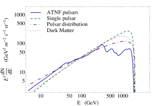
In Fig. 8 we compare the expected flux from a single pulsar (Sec. II), pulsars in the ATNF catalog (Sec. III), a continuous distribution of pulsars (Sec. III), and DM (Sec. IV). We have chosen the parameters of the models such that the fluxes have the same value at 100 GeV, similar indices at low energies, and a cutoff at 2 TeV. At energies below GeV, the fluxes are very similar. We also do not expect to see any differences between these models in the positron ratio below 300 GeV, the upper limit for charge identification in PAMELA.
Above 300 GeV, there are substantial differences among the spectrum predicted for these models. However, it should be noted that the sharpness of the cutoff for a single pulsar and for DM is strongly model dependent. If the injection cutoff for a pulsar is TeV, then the cutoff in the observed flux from a single pulsar can be much smoother than if the injection cutoff was higher than the cooling break, in which case its spectrum is indistinguishable from that predicted for a continuous distribution of pulsars. For the DM flux we show a model with only one intermediate particle in the annihilation-decay process. If there are more steps in the annihilation-decay process, then the flux has a broader cutoff and, again, may be impossible to distinguish between either a single pulsar or continuous pulsar distribution origin. Thus, given the significant uncertainties in the pulsar and DM models, it is unlikely that better observations alone can distinguish between a single pulsar and dark matter origin of anomalous flux Hall:2008qu (a similar conclusion was obtained in Ioka:2008cv Zhang:2008tb ).
The flux from a discrete collection of pulsars does have a few distinctive features at high energies. The height of these features is model dependent and may be within the error bars of current observations. The presence of these features requires the existence of a few young, nearby, energetic pulsars with an injection cutoff TeV. Consequently the absence of such features in the observed spectrum could mean that all young pulsars whose electrons have reached the Earth have had cutoffs TeV – a strong constraint on the properties of PWNe since, as we discuss in Appendix A, the PWN around the Vela pulsar has a cutoff in the electron and positron spectrum at an energy TeV. An additional smearing of the bumps can be due to spatial variations of the energy losses and the diffusion coefficient. Our general conclusion is that the current electron and positron data are not sufficient to distinguish between the pulsars and the dark matter and that independent measurements, e.g., the spectrum and morphology of the diffuse galactic gamma-ray background Zhang:2008tb ; Ando:2009fp , may be necessary in order to decisively distinguish a pulsar and DM origin of excess.
Acknowledgments. The authors are thankful Gregory Gabadadze, Andrei Gruzinov, Ignacy Sawicki, Jonathan Roberts, and Alex Vikman for valuable discussions. We are especially indebted to Neal Weiner for initiating the project and for numerous discussions and support during all stages of the work. This work is supported in part by the Russian Foundation of Basic Research under Grant No. RFBR 09-02-00253 (DM), by the NSF Grants No. PHY-0245068 (DM) and No. PHY-0758032 (DM), by DOE OJI Grant No. DE-FG02-06E R41417 (IC), by the NSF Astronomy and Astrophysics Postdoctoral Fellowship under Grant No. AST-0702957 (JG).
Appendix A Review of pulsars
In this appendix we review the emission of electrons from pulsars. We assume that this emission is powered by the pulsar’s loss of rotational energy. Pulsars are believed to be rotating neutron stars with a strong surface magnetic field Shapiro1983 , and magnetic dipole radiation is believed to provide a good description for its observed loss of rotational energy. A pulsar loses its rotational energy on a characteristic decay time defined as
| (41) |
where and are the initial rotational energy and the initial spin-down luminosity, respectively, which in the magnetic dipole radiation model are equal to
where is the initial angular velocity, is the radius of the pulsar, is the strength of the surface dipole magnetic field, and is the angle between the rotation axis and the magnetic field axis.
If the energy loss is due to magnetic dipole radiation, then
| (42) |
Integrating the energy loss equation we get
| (43) | |||||
| (44) |
As a result, the pulsar angular velocity satisfies
| (45) |
In a more general approach, the time evolution of the angular velocity is described as
| (46) |
where is the breaking index, which can be found by measuring the current , , and
| (47) |
In this case,
| (48) |
The magnetic dipole radiation corresponds to .
As an example, let us calculate the initial rotational energy of the Crab pulsar using the magnetic dipole approximation and a general braking index. The Crab pulsar is believed to have been produced during SN 1054 supernova explosion. Consequently, the age of the pulsar is known exactly, yr. In the magnetic dipole approximation, we can use Eq. (45) and the current values of and Manchester:2004bp ; 1993MNRAS.265.1003L to calculate that its pulsar time scale kyr. Assuming a mass , radius km, and moment of inertia Shapiro1983 , we derive an initial rotational energy erg. Taking into account the measured value of Manchester:2004bp , the braking index of the Crab pulsar is , which gives kyr and erg.
If the age of the pulsar is not known independently, it is impossible to determine and using its observed properties (from , , and one can only calculate ). In the following, we estimate by assuming kyr for all pulsars. If so, the initial energy can be found from Eq. (44) by using the current spin-down luminosity
| (49) |
For a general braking index , this formula takes the form
| (50) |
Using this method to estimate for all pulsars in the ATNF catalog results in the distribution shown in Fig. 9, using both the magnetic dipole approximation (Eq. (49)) and a general braking index method (Eq. (50)). In the magnetic dipole case we took all pulsars within 4 kpc from the Earth and younger than 300 kyr. The reason is that older and more distant pulsars are less luminous and may not be observed for small spin-down luminosities, i.e., this introduces a bias towards more energetic pulsars and shifts the distribution toward larger average . For the general braking index, we used all pulsars with . In both cases, can be described by a log-normal distribution with the average and the standard deviation . The average initial rotational energy in this case is
| (51) |
This result is strongly dependent on the chosen value of . For example, if kyr, then an analogous calculation gives , and erg. The estimations above agree with the analysis of FaucherGiguere:2005ny . It is worth noting that likely varies between pulsars.

To estimate , it is important to understand how the pulsar’s magnetic dipole radiation is transferred to the kinetic energy of particles. Since decays as , most of the rotational energy is lost at early times. A young pulsar is surrounded by several layers Rees:1974nr Kennel:1984vf . Nearest to the neutron star is the magnetosphere, which ends at the light cylinder . The rotating magnetic field creates a strong electric field capable of both producing pairs of particles and accelerating them to relativistic energies. These particles stream away from the light cylinder as a coherent “wind” that ends with a termination shock separating the wind zone from the PWN which consists of magnetic fields and particles moving in random directions. The PWN in turn is surrounded by an SNR. A significant PWN exists only at the early times ( kyr Gaensler:2006ua ).
The spectrum of electrons and positrons in the magnetosphere can be estimated using the spectrum of pulsed -ray emission from a pulsar. For the Crab pulsar, model fits to the observed photon spectrum suggest that the spectrum of pairs in its magnetosphere is well described by a broken power low with an index of below GeV and an index of between and an upper cutoff around GeV Harding:2008kk (see also Aliu:2008hc ). Particles with this spectrum cannot reproduce the spectrum observed on Earth, since a break in the injection spectrum at GeV is too low to explain the ATIC and PAMELA results, and an index of above 2 GeV also does not fit the data. Additionally, the pulsed emission from a pulsar only reflects the energy spectrum of the emitting particles in the emission region, which is not necessarily representative of the spectrum of particles that escape the pulsar magnetosphere along the open field lines and are eventually deposited in the ISM.
These particles are further accelerated before they enter the PWN, most likely at the termination shock between the magnetosphere and the PWN (for a review see, e.g., Arons1996 ). Once deposited in the PWN, they are trapped by the PWN’s magnetic field until it is disrupted. Observationally, the spectrum of the electrons inside the PWN is found by analyzing their broadband spectrum, which at low photon energies ( GeV) is dominated by synchrotron emission and at higher energies ( GeV) dominated by inverse Compton scattering of electrons off background photons 1996MNRAS.278..525A . From the radio spectrum of these objects, it is possible to constrain the spectral shape of the low energy (GeV) electrons which dominate by number the electron population of a PWN. An average index of the electron and positron spectrum can be found using data from the publicly available Catalogue of galactic SNRs Green:2009qf , where F-type (or “filled-center”) SNRs are PWNe, S-type are the supernova shells, and C-type SNRs are a combination of the two. There are 7 F-type SNRs with an average electron index . For 21 C-type SNRs the average index is , while 168 S-type SNRs have . It is clear that the spectrum of electrons in supernova shells is much softer (decreases faster with the energy) than the spectrum in PWNe. In order to explain the PAMELA positron ratio we need either F-type or, possibly, C-type SNRs because the S-type SNRs are produced by the initial supernova explosion and do not contain a significant number of positrons.
The broadband spectrum of most PWNe shows a break between the radio and X-ray regimes, believed to correspond to a break in the electron and positron spectrum, most likely the result of synchrotron cooling. Converting the frequency of this break to an electron/positron energy requires knowing the strength of the PWN’s magnetic field. An independent estimate of the magnetic field is available for those PWNe with detected inverse Compton emission, since this depends solely on the energy spectrum of electrons and positrons in the PWN and known properties of the various background photon fields (e.g., Cosmic Microwave Background and starlight). The best studied example is the Crab Nebula (e.g., 1996MNRAS.278..525A ), whose broadband photon spectrum suggests an electron spectrum well described by a broken power law with an index below GeV and between and an upper cutoff TeV: the magnetic field in this PWN has a strength of G, resulting in a ratio of magnetic energy flux to particle energy flux of 1996MNRAS.278..525A . For PWNe whose broadband spectrum is not as well determined, the break energy in the electron spectrum is typically derived using the minimum energy assumption ( Chevalier:2004rp ). Using this method and the observational data provided in Chevalier:2004rp , we estimate a break energy of GeV for the PWNe listed in this paper. It is important to emphasize that this procedure almost certainly overestimates the magnetic field strength inside a PWN since, for most PWNe, is believed to be . In this procedure, the inferred break energy is , where is the strength of PWN’s magnetic field. As a result, the true break energy of electrons and positrons inside the PWNe analyzed above is likely to be at least an order of magnitude higher than the derived value.
The break energy in the electron/positron spectrum of a PWN is expected to vary considerably during the lifetime of a PWN due largely to changes in the strength of the PWN’s magnetic field (e.g., Reynolds:1984 , Gelfand:2009aa ). Therefore, the break energy in the spectrum of electrons and positrons injected by the PWN into the surrounding ISM depends strongly on the evolutionary phase of the PWN when this occurs. During the initial free-expansion phase of the PWN’s evolution (the Crab Nebula is the prototypical example of such a PWN; Gaensler:2006ua ), the break energy is expected to increase as Reynolds:1984 ; Gelfand:2009aa . This phase of the PWN’s evolution ends when it collides with the SNR’s reverse shock, typically on the order of yr after the supernova explosion. If this holds for the Crab Nebula, its current age of yr and break energy of GeV suggests that, at the time of this collision, the break energy will have risen to TeV. The evolution of the break energy after this collision is more complicated and depends strongly on the properties of the central neutron star, progenitor supernova, and surrounding ISM (see Gelfand:2009aa for a more detailed discussion). There is observational evidence that the break energy of older PWNe ( yr old) is considerably higher than that of the Crab Nebula and other young PWNe ( yr). The most convincing example comes from a recent analysis of the broadband spectrum (radio to TeV rays) of the Vela PWN (often referred to as “Vela X”), which suggests a break in the electron spectrum of TeV Aharonian:2006xx . For the purpose of the work presented here, the exact value of the break is not important as far as it is bigger than TeV.
Observations indicate that most PWNe are particle dominated: i.e., almost of the spin-down luminosity is transformed into the energy of the particles after the termination shock. However, not all of this energy is eventually deposited in the ISM. We estimate this fraction, , by first assuming that the spectrum after the termination shock is a power law with an index and a cutoff TeV. Then, the total energy in electrons is
| (52) |
If, when the PWN is disrupted, the energy spectrum of electrons in the PWN is below the break at and with above the break, the total energy in electrons is saturated at with
| (53) |
The efficiency is therefore
| (54) |
For , TeV and TeV, this gives the suggested . This derivation should be viewed as an order of magnitude estimation. A more realistic calculation is extremely complicated and involves the knowledge of the PWN evolution and the actual spectra of particles inside a PWN. Recent work in this field does support an efficiency of (e.g., Gelfand:2009aa ).
It should be stressed that, apart from theoretical uncertainties, the parameters of the injection spectrum can vary significantly between pulsars. The initial rotational energy can differ by several orders of magnitude, while the index of the electron spectrum can vary from to . In some cases, it is observed to vary inside the PWN of a single pulsar. The upper cutoff , as we have seen in the examples of Crab and Vela pulsars, can vary at least between GeV and TeV.
Appendix B Spatial variation in energy losses
As we have discussed, an important signature of the flux from the pulsars is the presence of a number of bumps at the cooling break energies
| (55) |
where ’s are the ages of the pulsars. The existence of these bumps is based on the assumption that the energy losses depend only on the travel time and not their path. In reality, the energy loss coefficient depends on the position, since the densities of the star light and IR photons vary in space. In this case, there is no simple solution for Eq. (7), though one can still find the average energy loss and its standard deviation by averaging the energy losses over random paths.
As a useful simplification we will consider separately diffusion in space and energy losses. Our motivation is that a particle detected with energy has an energy close to during most of the propagation time (i.e. the cooling time from to is saturated by the final energy ). Consequently, the diffusion coefficient for all particles detected with energy can be approximated by . If so, the probability to propagate from a source at to an observer at is given by the Green function
| (56) |
In order to find the energy loss averaged over paths, it is useful to rewrite this Green function in terms of the path integral
| (57) |
where the action is
| (58) |
with the boundary conditions and .
In general, the average of a functional over paths is
| (59) |
Integrating the energy loss
| (60) |
along a path , we find
| (61) |
The functional that we will study is
| (62) |
The expression in the numerator of (59) is
| (63) | |||||
If we define , then all the paths can be represented as a path from to , the integral over all and the path from to :
| (65) | |||||
The resulting expression resembles the first order perturbation theory: there is a propagation from to , an insertion of an operator at and a propagation from to .
The average energy loss can be estimated with (65) and the Green function in (56). Taking in (61), we find that the average cooling break energy for a given pulsar is
| (66) | |||||
The standard deviation is
| (67) |
The average for the functional (62) can be computed analogously to (66)
where we assume that is at and is at . The factor of 2 is the usual for the time-ordered path integrals.
The relative standard deviation of the cooling break energy is
| (68) |
Using the energy densities of starlight and IR photons from Porter:2005qx we find the relative smearing in the energy
| (69) |
At 1 TeV the smearing is about 5%, at 100 GeV it is 11%, and at 10 GeV it is 24%. The flux from the ATNF pulsars with this smearing is shown in Fig. 4. At low energies the flux becomes very smooth but at high energies the bumps are still visible. We also notice that at high energies the relative width of the bumps is larger than the ratio in (69). Thus, even if the experimental energy resolution is about 10% – 15%, we should be able to see the bumps.
Appendix C Constraining pulsars and ISM properties
If we assume that the anomalies in Fermi, ATIC and PAMELA data are due to pulsars, we can use these results to constrain the properties of ISM and pulsars. The problem is that the flux depends on both the properties of the ISM and the injection spectrum from pulsars. As we discuss in Secs. II and III, the ISM can be described by three parameters , , and and the injection from a distribution of pulsars can be described by five parameters , , , , and . Obviously, the three parameters of the observed flux (the normalization, the index, and the cutoff) cannot constrain all eight parameters, but they can constrain some combinations of parameters. These constraints may be very useful if combined with results from other experiments, such as the observations of protons, heavy nuclei, or diffuse gamma rays.
Another concern is the reliability of constraints coming from the local flux. Ideally, we would like to constrain the parameters in the models, but since the local distribution of pulsars is fundamentally random in nature, there is a possibility that we can only constrain the properties of particular pulsars without getting any information about the general population. The reason why we think our approach is sensible is the following. At high energies, the flux from pulsars will depend significantly on the properties of individual pulsars (and we can use this region to prove that the observed flux is due to pulsars), but at low energies the flux is well approximated by the continuous distribution flux and the properties of individual pulsars are relatively unimportant. Thus, we propose using the observed spectrum at intermediate energies as a testing ground to study the general (or averaged) properties of injection from pulsars.
In the following we will fit the continuous distribution flux derived in Eq. (27) to the Fermi and PAMELA data simultaneously. In these fits we substitute the usual pulsar injection cutoff TeV by the propagated (or statistical) cutoff and treat it as a fit parameter. The other fit parameters are (these values are based on the energy densities of radiation and magnetic field within few kpc from the Earth), Strong:2007nh . The injection index and the conversion efficiency erg are discussed in Appendix A. In the fits we use , and . The best-fit parameters are: , = , = erg, , and TeV. The corresponding fluxes are shown in Fig. 6.

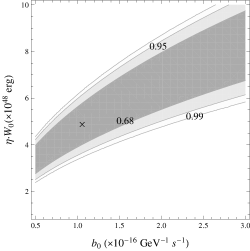
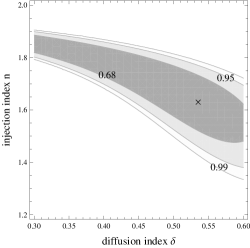

In Fig. 10 we plot the , and CL of these parameters. Every contour plot is obtained by varying two parameters while keeping the rest fixed at their best-fit value. We can see that for any value of the energy loss coefficient within the region chosen, there is a value of diffusion index that can provide a fit within CL. Additionally, a higher value of suggests a lower value of , in agreement with the calculation of the flux from a continuous distribution of pulsars where we expect that from Eq. (27). Assuming a high value for the injection index (), the Fermi and PAMELA data could be fitted by a relatively large region of values of the propagation parameters ( and ). On the other hand, values of do not seem to give a very good fit to the data, with any combination of propagation parameters. Also if the total energy converted to is smaller than erg, then for a pulsar birth rate of 1.8 per kyr regardless of the value of the Fermi and PAMELA data cannot be explained by the continuous distribution of pulsars.
| Pulsar | ||||
|---|---|---|---|---|
| Distribution | ||||
| Cont. dist. B1 | 0.5-3.0 | 0.30-0.60 | 1.35-1.95 | 0.025-0.11 |
| Cont. dist. B2 | 0.5-3.0 | 0.30-0.60 | 1.40-1.95 | 0.020-0.085 |
| 4kpc pulsars B1 | 0.5-2.4 | 0.30-0.60 | 1.25-1.80 | 0.025-0.14 |
| 4kpc pulsars B2 | 0.5-2.0 | 0.30-0.60 | 1.15-1.95 | 0.020-0.13 |
To show the robustness of our procedure we applied the same analysis for two different backgrounds, a power law background (B1) and a more conventional background used in Abdo:2006fq (B2). In Table I, we present the C.L. allowed region of values of the averaged ISM and averaged pulsar properties, using the two different backgrounds for the continuous pulsar distribution used. Alternatively, we used the properties of pulsars in the ATNF database with estimated distances kpc. We present in Table I the derived constraints in the ISM averaged properties and universal pulsar properties and .
Better data on the flux of the high energy and on the pulsar birth rate will make this analysis more successful in confining the parameter space that is relevant for the pulsar scenario. Tighter constraints of the backgrounds and the parameters of propagation through the ISM will be needed to confine the properties of pulsars themselves.
References
- (1) J. Chang et al., “An excess of cosmic ray electrons at energies of 300.800 GeV,” Nature 456 (2008) 362–365.
- (2) O. Adriani et al., “Observation of an anomalous positron abundance in the cosmic radiation,” arXiv:0810.4995 [astro-ph].
- (3) H.E.S.S. Collaboration, F. Aharonian et al., “The energy spectrum of cosmic-ray electrons at TeV energies,” Phys. Rev. Lett. 101 (2008) 261104, arXiv:0811.3894 [astro-ph].
- (4) H.E.S.S. Collaboration, F. Aharonian et al., “Probing the ATIC peak in the cosmic-ray electron spectrum with H.E.S.S,” arXiv:0905.0105 [astro-ph.HE].
- (5) The Fermi LAT Collaboration, A. A. Abdo et al., “Measurement of the Cosmic Ray e+ plus e- spectrum from 20 GeV to 1 TeV with the Fermi Large Area Telescope,” arXiv:0905.0025 [astro-ph.HE].
- (6) I. Cholis, L. Goodenough, and N. Weiner, “High Energy Positrons and the WMAP Haze from Exciting Dark Matter,” arXiv:0802.2922 [astro-ph].
- (7) L. Bergstrom, T. Bringmann, and J. Edsjo, “New Positron Spectral Features from Supersymmetric Dark Matter - a Way to Explain the PAMELA Data?,” Phys. Rev. D78 (2008) 103520, arXiv:0808.3725 [astro-ph].
- (8) M. Cirelli, M. Kadastik, M. Raidal, and A. Strumia, “Model-independent implications of the e+, e-, anti-proton cosmic ray spectra on properties of Dark Matter,” arXiv:0809.2409 [hep-ph].
- (9) I. Cholis, L. Goodenough, D. Hooper, M. Simet, and N. Weiner, “High Energy Positrons From Annihilating Dark Matter,” arXiv:0809.1683 [hep-ph].
- (10) N. Arkani-Hamed, D. P. Finkbeiner, T. Slatyer, and N. Weiner, “A Theory of Dark Matter,” (2008) , arXiv:0810.0713 [hep-ph].
- (11) P.-f. Yin et al., “PAMELA data and leptonically decaying dark matter,” arXiv:0811.0176 [hep-ph].
- (12) K. Hamaguchi, E. Nakamura, S. Shirai, and T. T. Yanagida, “Decaying Dark Matter Baryons in a Composite Messenger Model,” arXiv:0811.0737 [hep-ph].
- (13) C.-R. Chen, K. Hamaguchi, M. M. Nojiri, F. Takahashi, and S. Torii, “Dark Matter Model Selection and the ATIC/PPB-BETS anomaly,” arXiv:0812.4200 [astro-ph].
- (14) T. Kobayashi, Y. Komori, K. Yoshida, and J. Nishimura, “The most likely sources of high energy cosmic-ray electrons in supernova remnants,” Astrophys. J. 601 (2004) 340–351, arXiv:astro-ph/0308470.
- (15) D. Hooper, P. Blasi, and P. D. Serpico, “Pulsars as the Sources of High Energy Cosmic Ray Positrons,” JCAP 0901 (2009) 025, arXiv:0810.1527 [astro-ph].
- (16) H. Yuksel, M. D. Kistler, and T. Stanev, “TeV Gamma Rays from Geminga and the Origin of the GeV Positron Excess,” arXiv:0810.2784 [astro-ph].
- (17) S. Profumo, “Dissecting Pamela (and ATIC) with Occam’s Razor: existing, well-known Pulsars naturally account for the ’anomalous’ Cosmic-Ray Electron and Positron Data,” arXiv:0812.4457 [astro-ph].
- (18) K. Ioka, “A Gamma-Ray Burst for Cosmic-Ray Positrons with a Spectral Cutoff and Line,” arXiv:0812.4851 [astro-ph].
- (19) F. A. Aharonian, A. M. Atoyan, and H. J. Voelk, “High energy electrons and positrons in cosmic rays as an indicator of the existence of a nearby cosmic tevatron,” Astron. Astrophys. 294 (1995) L41–L44.
- (20) M. J. Rees and J. E. Gunn, “The origin of the magnetic field and relativistic particles in the Crab Nebula,” Mon. Not. Roy. Astron. Soc. 167 (1974) 1–12.
- (21) P. A. Caraveo, G. F. Bignami, A. DeLuca, S. Mereghetti, A. Pellizzoni, R. Mignani, A. Tur, and W. Becker, “Geminga’s Tails: A Pulsar Bow Shock Probing the Interstellar Medium,” Science 301 (2003) 1345–1348.
- (22) G. G. Pavlov, D. Sanwal, and V. E. Zavlin, “The pulsar wind nebula of the Geminga pulsar,” Astrophys. J. 643 (2006) 1146–1150, arXiv:astro-ph/0511364.
- (23) B. M. Gaensler et al., “The Mouse That Soared: High Resolution X-ray Imaging of the Pulsar-Powered Bow Shock G359.23-0.82,” Astrophys. J. 616 (2004) 383–402, arXiv:astro-ph/0312362.
- (24) B. M. Gaensler and P. O. Slane, “The Evolution and Structure of Pulsar Wind Nebulae,” Ann. Rev. Astron. Astrophys. 44 (2006) 17–47, arXiv:astro-ph/0601081.
- (25) C. F. Kennel and F. V. Coroniti, “Confinement of the Crab pulsar’s wind by its supernova remnant,” Astrophys. J. 283 (1984) 694.
- (26) J. Hall and D. Hooper, “Distinguishing Between Dark Matter and Pulsar Origins of the ATIC Electron Spectrum With Atmospheric Cherenkov Telescopes,” arXiv:0811.3362 [astro-ph].
- (27) FERMI-LAT Collaboration, D. Grasso et al., “On possible interpretations of the high energy electron- positron spectrum measured by the Fermi Large Area Telescope,” arXiv:0905.0636 [astro-ph.HE].
- (28) R. N. Manchester, G. B. Hobbs, A. Teoh, and M. Hobbs, “The ATNF Pulsar Catalogue,” arXiv:astro-ph/0412641. http://www.atnf.csiro.au/research/pulsar/psrcat.
- (29) M. S. Longair, High-energy astrophysics. Cambridge University Press, Cambridge, England, 1992.
- (30) A. W. Strong, I. V. Moskalenko, and V. S. Ptuskin, “Cosmic-ray propagation and interactions in the Galaxy,” Ann. Rev. Nucl. Part. Sci. 57 (2007) 285–327, arXiv:astro-ph/0701517.
- (31) T. A. Porter and A. W. Strong, “A new estimate of the Galactic interstellar radiation field between 0.1 microns and 1000 microns,” arXiv:astro-ph/0507119.
- (32) V. L. Ginzburg and S. I. Syrovatskii, The Origin of Cosmic Rays. Pergamon, Oxford, 1964.
- (33) S. I. Syrovatskii, “The Distribution of Relativistic Electrons in the Galaxy and the Spectrum of Synchrotron Radio Emission,” Astr. Zh. 36 (1959) 17.
- (34) S. L. Shapiro and S. A. Teukolsky, Black Holes, White Dwarfs, and Neutron Stars. Wiley, New York, 1983.
- (35) C.-A. Faucher-Giguere and V. M. Kaspi, “Birth and Evolution of Isolated Radio Pulsars,” Astrophys. J. 643 (2006) 332–355, arXiv:astro-ph/0512585.
- (36) F. A. Aharonian and A. M. Atoyan, “On the mechanisms of gamma radiation in the Crab Nebula,” Mon. Not. Roy. Astron. Soc. 278 (1996) 525–541.
- (37) D. Malyshev, “On discrepancy between ATIC and Fermi data,” arXiv:0905.2611 [astro-ph.HE].
- (38) G. Bertone, D. Hooper, and J. Silk, “Particle dark matter: Evidence, candidates and constraints,” Phys. Rept. 405 (2005) 279–390, arXiv:hep-ph/0404175.
- (39) M. Kuhlen and D. Malyshev, “ATIC, PAMELA, HESS, Fermi and nearby Dark Matter subhalos,” arXiv:0904.3378 [hep-ph].
- (40) M. Pohl, “Cosmic-ray electron signatures of dark matter,” arXiv:0812.1174 [astro-ph].
- (41) D. Hooper, A. Stebbins, and K. M. Zurek, “The PAMELA and ATIC Excesses From a Nearby Clump of Neutralino Dark Matter,” arXiv:0812.3202 [hep-ph].
- (42) I. Cholis, G. Dobler, D. P. Finkbeiner, L. Goodenough, and N. Weiner, “The Case for a 700+ GeV WIMP: Cosmic Ray Spectra from ATIC and PAMELA,” arXiv:0811.3641 [astro-ph].
- (43) J. Hisano, M. Kawasaki, K. Kohri, and K. Nakayama, “Neutrino Signals from Annihilating/Decaying Dark Matter in the Light of Recent Measurements of Cosmic Ray Electron/Positron Fluxes,” arXiv:0812.0219 [hep-ph].
- (44) J. Liu, P.-f. Yin, and S.-h. Zhu, “Prospects for Detecting Neutrino Signals from Annihilating/Decaying Dark Matter to Account for the PAMELA and ATIC results,” arXiv:0812.0964 [astro-ph].
- (45) J. Zhang et al., “Discriminate different scenarios to account for the PAMELA and ATIC data by synchrotron and IC radiation,” arXiv:0812.0522 [astro-ph].
- (46) S. Ando, “Gamma-ray background anisotropy from galactic dark matter substructure,” arXiv:0903.4685 [astro-ph.CO].
- (47) A. G. Lyne, R. S. Pritchard, and F. G. Smith, “23 years of Crab pulsar rotational history,” MNRAS 265 (1993) 1003–1012.
- (48) A. K. Harding, J. V. Stern, J. Dyks, and M. Frackowiak, “High-Altitude Emission from Pulsar Slot Gaps: The Crab Pulsar,” arXiv:0803.0699 [astro-ph].
- (49) The MAGIC Collaboration, E. Aliu et al., “Detection of pulsed gamma-ays above 25 GeV from the Crab pulsar,” arXiv:0809.2998 [astro-ph].
- (50) J. Arons, “Pulsars as Gamma-Rays Sources: Nebular Shocks and Magnetospheric Gaps,” Space Sci. Rev. 75 (1996) 235–255.
- (51) D. A. Green, “A Revised Galactic Supernova Remnant Catalogue,” arXiv:0905.3699 [astro-ph.HE]. to appear in the Bulletin of the Astronomical Society of India.
- (52) R. A. Chevalier, “Young core collapse supernova remnants and their supernovae,” Astrophys. J. 619 (2005) 839–855, arXiv:astro-ph/0409013.
- (53) S. P. Reynolds and R. A. Chevalier, “Evolution of pulsar-driven supernova remnants,” Astrophys. J. 278 (1984) 630–648.
- (54) J. D. Gelfand, P. O. Slane, and W. Zhang, “A Dynamical Model for the Evolution of a Pulsar Wind Nebula inside a Non-Radiative Supernova Remnant,” arXiv:0904.4053 [astro-ph.HE].
- (55) H.E.S.S. Collaboration, F. Aharonian et al., “First detection of a VHE gamma-ray spectral maximum from a Cosmic source: H.E.S.S. discovery of the Vela X nebula,” Astron. Astrophys. 448 (2006) L43–L47, arXiv:astro-ph/0601575.
- (56) A. A. Abdo et al., “Discovery of TeV gamma-ray emission from the Cygnus region of the galaxy,” Astrophys. J. 658 (2007) L33–L36, arXiv:astro-ph/0611691.