Detecting Transits in Sparsely Sampled Surveys

Abstract

The small sizes of low mass stars in principle provide an opportunity to find Earth-like planets and “super Earths” in habitable zones via transits. Large area synoptic surveys like Pan-STARRS and LSST will observe large numbers of low mass stars, albeit with widely spaced (sparse) time sampling relative to the planets’ periods and transit durations. We present simple analytical equations that can be used to estimate the feasibility of a survey by setting upper limits to the number of transiting planets that will be detected. We use Monte Carlo simulations to find upper limits for the number of transiting planets that may be discovered in the Pan-STARRS Medium Deep and 3$\pi$ surveys. Our search for transiting planets and M-dwarf eclipsing binaries in the SDSS-II supernova data is used to illustrate the problems (and successes) in using sparsely sampled surveys.

1 Planets Orbiting Low Mass Stars

Planets transiting low mass (M $\leq$ 0.6 M_⊙) stars are important for many reasons. To $\sim$10% accuracy, the radii of stars with M $\leq$ 1 M_⊙ are $R_{star}/R_{\odot}\sim M_{star}/M_{\odot}$. Consequently, it is easier for ground based telescopes to detect planets of all sizes, especially Neptune-sized ice-giant planets, around M-dwarfs. Table 1 illustrates this point by showing the ratio of geometrical transit depths expressed as magnitudes of Jupiter, Neptune, and the Earth transiting stars of different masses. The radii of the stars were calculated using $R_{star}/R_{\odot}=0.927\times M_{star}/M_{\odot}+0.037\pm 0.02$, which is a linear fit to the masses and radii of 38 low mass stars (see Lop05 ; Heb06 ; Pon06 ; Bou05 ; Del99 ; Del00 ; Lan02 ).

$\mathbf{M_{star}/M_{\odot}}$	$\mathbf{R_{star}/R_{\odot}}$	Spectral Type	$\mathbf{M_{i^{*}}/M_{z^{*}}}$	Jupiter	Neptune	Earth
1.00	1.00	G2	-	0.011	0.001	0.0001
0.65	0.64	M0	8.4/7.9	0.028	0.003	0.0002
0.45	0.45	M2	8.9/8.3	0.057	0.005	0.0004
0.15	0.18	M4	10.7/9.9	0.447	0.036	0.0029
0.092	0.12	M6	13.2/11.9	1.299	0.076	0.0061
0.079	0.11	M8	14.9/13.2	2.118	0.094	0.0075

Table 1: Radii, Spectral type, and geometric transit depth in magnitudes of transits for planets as a function of the mass of the parent star.

With a limit of $\sim$2 mmag light-curve precision, transiting Neptune-sized planets are very difficult to detect via transits around main sequence G-dwarf host stars, even in the best ground-based photometric data. However, a Neptune-sized planet orbiting a 0.4 M_⊙ M-dwarf has a detectable transit with a depth of 0.036 mag, and becomes more detectable as the host mass decreases. Observing these transits around M-dwarfs will yield the radii of Neptune-like planets and rocky planets. These radii, combined with radial velocity measurements, determine the planets’ densities, and thus provide important information about their mean composition. Reflected and emitted light measurements, in addition to transmission spectra, constrain the physics and composition of planetary atmospheres.

2 Estimating the Number of Planets Transiting Low Mass Stars in a Given Survey

We will show why large area surveys are needed to find appreciable numbers of planets transiting low mass stars by beginning with some simple geometrical considerations. Defining the inclination of the planet’s orbit as the angle between the line of sight and the orbital plane, the critical angle for a transit to occur is

$$\sin\theta_{c}=(R_{s}+R_{p})/R$$ (1)

where $R_{s}$ and $R_{p}$ are the radii of the star and planet respectively, and R is the radius of the circular orbit. If there are $N_{p}$ planet bearing stars with randomly oriented orbits, the number of stars with planets that can transit (as opposed to the number that will be observed), is

$$N_{0}=N_{p}(R_{s}+R_{p})/R,$$ (2)

showing the strong selection for short period planets. The number of planets $N_{I}$ transiting at any given instant is $N_{p}$ times the fractional area of a circle with radius $R_{s}+R_{p}$ projected onto a sphere of radius $R$, and is given by the equation

$$N_{I}=N_{p}\times(1/2)(1-\cos\theta_{c}).$$ (3)

Equation 3 is easily understood by thinking of the projection of $R_{s}+R_{p}$ onto a sphere with radius R as a “polar cap”, with the line of sight along the axis of the pole.

We can now estimate the number $N_{t}$ of planets that can possibly transit during a continuous observation time $t_{obs}$ that is less than half the planet’s period by first considering an observation time $t_{1/4}$ that lasts for 1/4 of a period. If we suppose that all of the transiting planets have zero inclination, then half of the planets $N_{0}$ can reach the polar cap and transit, and half of this number will have an orbit toward the polar cap, and in fact transit. Consequently,

$$N_{t}\approx\left(N_{p}/4\right)(R_{s}+R_{p})/R.$$ (4)

Because not all transiting planets have zero inclination, Equation 4 is an upper limit to the number of transits that will be observed, and becomes a progressively better estimate as the critical angle $\theta_{c}$ becomes smaller (i.e. as the period increases for a fixed stellar mass). Taking into account the fraction of planets that project onto the polar cap, an approximate upper limit for the number of planets that are transiting or will transit during $t_{obs}$ is

$$N_{t}=\frac{N_{p}}{2}\left[\left(\frac{R_{s}+R_{p}}{R}\right)\left(\frac{\cos\theta_{c}-\cos\theta_{t}}{2}\right)+(1-\cos\theta_{c})\right]$$ (5)

where the angle $\theta_{t}$ is given by

$$\theta_{t}=\theta_{c}+2\pi t_{obs}/\mathrm{Period}.$$ (6)

We next estimate the number of stars $N(D,l,b)$ that will be in a survey area $d\Omega$ to distance $D$ corresponding to a limiting magnitude $m_{lim}$. Although the density of stars is a function of Galactic longitude and latitude, M-dwarfs are faint enough that, depending on $m_{lim}$, only a few hundred parsecs will be sampled. Consequently, for a first order model, we can assume an exponential density as a function of Galactic latitude. The number of stars is then

$$N(D,b)=N_{0}(m_{1},m_{2})d\Omega\int_{0}^{D}r^{2}e^{-\frac{r\sin b}{r_{0}}}dr$$ (7)

where $N_{0}(m_{1},m_{2})$ is the density of stars of a particular type in the galactic plane, and $r_{0}$ is the scale height perpendicular to the plane. To calculate $N_{0}(m_{1},m_{2})$ we assume a mass function of the form

$$\frac{dN}{dM}=0.0187m^{-\alpha}\mathrm{stars\ pc^{-3}}$$ (8)

where the normalization and coefficient $\alpha=1.3$ are taken from Reid et al. Rei02 . The equation integrates to give

$$N_{0}(m_{1},m_{2})=\frac{0.0187}{1-\alpha}\left(m_{2}^{1-\alpha}-m_{1}^{1-\alpha}\right)\mathrm{stars\ pc^{-3}}.$$ (9)

We now use the preceding equations to estimate how many M-dwarfs of a given type will be in a particular survey. As an example, consider stars with masses between 0.1375 and 0.175 M_⊙, corresponding to a mean spectral type of M4. Using Equation 9, the space density of M4 stars is $\sim 0.008\ \mathrm{stars\ pc^{-3}}$; if the 5$\sigma$ limiting magnitude is $z^{*}=21.0$, the limiting distance is $\sim$1700 pc, and there are $\sim$1300 M4 stars/sq-deg at $b=15$ deg. However, we show in the next section that detection of Neptune-sized objects with a SNR of 5 in a single observation requires decreasing the 5$\sigma$ limiting magnitude by 3.6 mags to $z^{*}=17.4$, dropping the number of M4 stars to $\sim$300 per sq-deg. If we assume 1 hour of continuous observing and that all of the planets are Neptune-like in a $\sim$2 day orbit, the fraction of planets that can transit (Equation 2) is 0.05, and the fraction that will transit (Equations 5 and 6) is $6.2\times 10^{-4}$. If we make the optimistic assumption that 10% of all M4 stars have short-period planets, the probability that a transit occurs during a 1 hour observation is $6.2\times 10^{-5}$ per planet bearing star. We must survey nearly 55 sq-deg for an hour to detect just one transiting planet!

Surveying at low Galactic latitudes increases the number of M4 stars by an order of magnitude, at the price of decreasing the photometric accuracy because of crowding, and greatly increasing the number of false positives from blends of single stars with the target variable stars. Calculations show that observing at infrared wavelengths where the M dwarfs are much brighter helps very little from the ground because the gains from increased luminosities are completely offset by the increases in sky background.

We look at the prospects of finding planets transiting low mass stars in sparsely sampled, wide area surveys below.

3 The Pan-STARRS-1 Survey

The prototype telescope for the Panoramic Survey Telescope and Rapid Response System (Pan-STARRS), PS1, is presently being commissioned at the Haleakala Observatories in Hawaii. Three PS1 programs are relevant for finding transiting planets. The first, Pan-Planets Afo07 , consists of 3 campaigns of $i$-band bright time imaging of several adjacent fields in the Galactic bulge, the Hyades, and in Praesepe. The Galactic bulge fields will include $\sim$480,000 dwarf stars to a limiting magnitude of $i=17.0$; $\sim$100 short period transiting Jupiter-sized planets are expected to be found. The host stars will be bright enough for the planets to be confirmed by radial velocity observations. Unfortunately, the small number of M-dwarfs in these fields ($\sim$15,000; Afo07 ) brighter than the limiting magnitude will lead to very few detections of Jupiter and Neptune-sized planets around these stars.

The second of these programs, the PS1 Medium Deep Survey (MDS), will survey up to 7 fields (one field is 7 sq-deg) every usable night, covering a total of 10 fields in a year. Each field will be observed in g and r, i, z, and y over the course of four nights. Assuming $65\%$ of the nights are clear, the cycle of five filters in four nights will be repeated 35 times per year for three years. The $5\sigma$ limiting magnitudes for an $i$-band exposure on a single night is given in Table 2. The PS1 goal for absolute photometry precision is 0.01 mag. To detect the 0.036 mag depth (0.033 in flux) of a Neptune transiting an M4 star in a single observation, the photometric noise in the star must be $\leq$ 0.007 mags. Assuming that differential photometry will meet this requirement, the magnitude cutoff for the survey must be decreased by 3.6 magnitudes. The average of the estimated number of M-dwarfs with masses $\leq$ 0.175 M_⊙ ($\sim$M3.5) in the MDS $i$-band and $z$-band images is $\sim 24,000$. To first order the average of the numbers in the $r$ and $y$ filters will be comparable. The majority of the stars will have spectral types between M3.5 and M5. Taking $\mathrm{M}=0.1375\mathrm{M}_{\odot}$ ($\sim$M4.5) as representative of these stars and assuming all of them have a Neptune-sized planet with a period drawn from a uniform random distribution of periods between 1 and 3 days, a Monte Carlo simulation of three years of observations gives the transits listed in Table 2.

Survey	Filter	Num. Obs./ Field/Year	Obs. Sep. Nights	Survey Limit ($5\sigma$)	Survey Limit ($140\sigma$)	Num. of Stars	Trans. Planets	Avg. Num. Trans/Star
MDS	$r,i,z,y$	$\sim$ 140	1	25.4	21.8	$\sim$24,000	$<$ 120	10.0
3$\mathrm{\pi}$	$i$	2	30	23.35	19.7	$9.7\times 10^{6}$	$<$ 4,000	1.04
3$\mathrm{\pi}$	$z$	2	30	23.35	18.7	$8.3\times 10^{6}$	$<$ 3,400	1.04

Table 2: Estimated upper limits to the number of detectable planets transiting low mass stars in the Pan-STARRS MDS and 3$\pi$ surveys. Columns 1–6 describe the assumed cadence for the MDS and $3\pi$ surveys, the $5\sigma$ limiting magnitudes for a single exposure, and the $140\sigma$ limits for a $5\sigma$ detection of a Neptune-sized planet transiting an M4 dwarf. The last three columns give the number of stars in the respective survey areas to the $140\sigma$ limit, the number of planets that will transit if $10\%$ of these stars have a Neptune-sized planet in an orbit with a period drawn from a uniform random distribution between 1 and 3 days, and the average number of transits per star.

Even if we assume that 10% of all late M-dwarfs have a short period Neptune-sized planet, the MDS numbers are relatively small, given that only a fraction of planets that do transit during an observation will be detected in the face of random noise, red noise, blending with eclipsing binaries or variable stars, and other effects. The good news is that there should be $\sim$ 10 transits per short period transiting planet in the MDS survey, which will increase their detectability.

Table 1 shows that transiting Jupiter-sized planets are far more detectable around the earlier and brighter M-dwarfs than Neptune-sized planets. Gaudi Gau07 concludes that $\sim$40 such planets may be found by the MDS. This estimate, however, depends on the unknown frequency of such higher mass planets around M-dwarfs.

The final PS1 program that we consider, the $3\pi$ steradian survey, will observe the entire sky visible from Hawaii approximately once a week. Each field will be observed 4 times a year in each of the five filters for 3 years (60 epochs in all filters). Each night that a field is observed in a particular filter, the field will be observed twice with a separation of 30–60 minutes to identify moving solar system objects. We (arbitrarily) assume that the observations two nights per year for each filter per field will be separated by 30 days, and the transits observed in the $i$ and $z$ images are for different stars. A Monte Carlo simulation spanning three years yields the numbers given in Table 2. Again, assuming that 10% of all low mass M-dwarfs have short period Neptune-sized planets, the $3\pi$ survey could yield $\sim$ 300 such stars with 2 possible transits each. Detecting planets which transit only twice during widely separated short observation will be very difficult. Unless the cadence between the  r,i,z,y filters is optimized for detecting transits in the $3\pi$ survey, few planets transiting low mass stars will be detected.

Another issue that must be addressed is stellar activity in fast-rotating, fully convective low mass dwarfs. Two recent encouraging photometric campaigns on the young active M1Ve star AU Mic demonstrated that the star’s flare activity, its 4.85 day rotation, and variability due to two large star spots, did not prevent differential photometry accurate to a few mmag Heb07 . A modest photometric study of late M-dwarfs could be used to assess the limits on transit detection set by stellar activity. The next step is to make more realistic simulations that include noise sources, specific detection algorithms, and search for optimal survey cadences.

4 The SDSS-II Supernova Survey

The SDSS-II Supernova Survey Fri08 , in its three years of operation, monitored an $\sim$300 sq-deg area on the Celestial Equator known as SDSS Stripe 82 for three months per season, with a rough cadence of one observation every two nights. We used photometric catalogs from the Survey to search for low mass M-dwarf binaries and transiting planets. We extracted objects that were classified as stars with clean photometry and enforced an upper magnitude limit of $z=21.0$ mag. We then matched detections of objects across all three seasons to build up an extensive light-curve catalog.

From this catalog, we selected objects that had $\geq$ 10 observations over the three seasons, leaving us with approximately 1.1 million point sources. We used ensemble photometry techniques Hon92 to generate differential magnitude light-curves, thus decreasing the chance of incorrectly flagging an object as periodically variable if its light-curve was affected by the systematic artifacts caused by changing sky conditions and/or small changes in photometric zero points. We obtained an average photometric precision of about 30 mmag at $i=19.0$ mag, which effectively rules out the possibility of finding transiting planets around low mass stars, but is comfortably within the detection regime of M-dwarf eclipsing binaries.

We used SDSS $r-i$ and $i-z$ color cuts defined by West et al. Wes05 to select $\sim$690,000 likely M-dwarfs from our sample of 1.1 million point sources limited to $z=21.0$ mag. To find periodic variables, we employed the Stetson variability index Ste96 ; this removed from consideration a large number of faint objects that appeared to be variable because of photometric noise. We then inspected the differential magnitude light-curves of color-selected likely M-dwarfs that survived this selection process, looking for multi-band events that were eclipse-like.

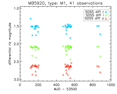
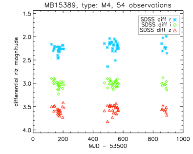
Figure 1: Differential photometry $riz$ light-curves for two M-dwarf eclipsing binary candidates from the SDSS-II Supernova Survey: MB5920 (left panel) and MB15389 (right panel). The differential magnitudes have been shifted on the y-axis for clarity. Both candidate names are internal designations.

A rough estimate of the total number $N_{det}$ of eclipsing binary M-dwarf systems we expect to find is given by

$$N_{det}=N_{*}\times f_{M}\times f_{bin}(P)\times f_{trans}\times f_{thresh}.$$ (10)

$N_{*}$ is the total number of stars in our sample, $f_{M}$ is the fraction of M-dwarfs seen in the sample, $f_{bin}(P)$ is the M-dwarf binary fraction as a function of period, $f_{trans}$ is the fraction of M-dwarf binary systems that can be observed by our survey, and $f_{thresh}$ is the fraction of M-dwarf eclipsing binary systems that will be detected given our survey’s SNR and throughput limits. Using the numbers from our sample for $N_{*}\simeq 1.1\times 10^{6}$, $f_{M}\simeq 0.60$, and conservative estimates for $f_{bin}(\mathrm{2.5-7\ days})\simeq 0.01$, $f_{trans}\simeq 0.05$, and $f_{thresh}\simeq 0.05$, we estimate that we may be able to find up to 17 M-dwarf eclipsing binaries.

To date, we have processed $\sim$30% of our sample and have found 12 candidates. We present the light-curves of two such objects in Figure 1. We are currently testing various period-finding techniques, including BLS Kov02 , and AoV Sch96 , to determine the likely periods of these systems. This will allow us to generate ephemerides for photometric monitoring, and enable eventual radial velocity followup to confirm whether they are indeed eclipsing binary systems of low mass M-dwarfs.

References

- (1) M. López-Morales and I. Ribas, ApJ 631, 1120 (2005)
- (2) L. Hebb et al., AJ 131, 555 (2006)
- (3) F. Pont et al., A&A 447, 1035 (2006)
- (4) F. Bouchy et al., A&A 431, 1105 (2005)
- (5) X. Delfosse et al., A&A 341, 63L (1999)
- (6) X. Delfosse et al., A&A 364, 217 (2000)
- (7) B. F. Lane et al., A&A 551, 81L (2001)
- (8) I. N. Reid et al., AJ 124, 2721 (2002)
- (9) C. Afonso and T. Henning, ASPC 366, 326A (2007)
- (10) S. Gaudi, ASPC 366, 273 (2007)
- (11) L. Hebb et al., MNRAS 379, 63 (2007)
- (12) J. A. Frieman et al., AJ 135, 338 (2008)
- (13) R. K. Honeycutt, PASP 104, 435 (1992)
- (14) A. A. West et al., PASP 117, 106 (2005)
- (15) P. B. Stetson, PASP 108, 851 (1996)
- (16) G. Kovács, S. Zucker, T. Mazeh A&A 391, 369 (2002)
- (17) A. Schwarzenberg-Czerny, ApJ 460, L107 (1996)