Thermodynamics of layered Heisenberg magnets with arbitrary spin

Abstract

We present a spin-rotation-invariant Green-function theory of long- and short-range order in the ferro- and antiferromagnetic Heisenberg model with arbitrary spin quantum number $S$ on a stacked square lattice. The thermodynamic quantities (Curie temperature $T_{C}$, Néel temperature $T_{N}$, specific heat $C_{V}$, intralayer and interlayer correlation lengths) are calculated, where the effects of the interlayer coupling and the $S$ dependence are explored. In addition, exact diagonalizations on finite two-dimensional (2D) lattices with $S\geqslant 1$ are performed, and a very good agreement between the results of both approaches is found. For the quasi-2D and isotropic 3D magnets, our theory agrees well with available quantum Monte Carlo and high-temperature series-expansion data. Comparing the quasi-2D $S=1/2$ magnets, we obtain the inequalities $T_{N}>T_{C}$ and, for small enough interlayer couplings, $T_{N}<T_{C}$. The results for $C_{V}$ and the intralayer correlation length are compared to experiments on the quasi-2D antiferromagnets Zn₂VO(PO₄)₂ with $S=1/2$ and La₂NiO₄ with $S=1$, respectively.

I INTRODUCTION

Low-dimensional ferromagnetic (FM) and antiferromagnetic (AF) quantum spin systems,SRF04 such as the quasi-two-dimensional (2D) Heisenberg ferromagnets [e.g., K₂CuF₄ with spin $S=1/2$ (Ref. LPS87, )] and antiferromagnets [e.g., La₂NiO₄ with spin $S=1$ (Ref. NYH95, ) being isostructural to the high-$T_{C}$ parent compound La₂CuO₄], are of current interest. Their study is motivated by the progress in the synthesis of new low-dimensional materials. For example, very recently a defective graphene sheet was reported to be a room-temperature ferromagnetic semiconductor that may be described by an effective quasi-2D Heisenberg model.PMH08

Investigations of layered Heisenberg magnets by numerical methods, e.g., quantum Monte Carlo (QMC) simulations and high-temperature series expansions (SE), have been performed for a selected number of cases and quantities only. QMC data are available for quasi-2D and spatially isotropic 3D antiferromagnets with $S=1/2$ (Refs. SSS03, ; YTH05, ; San98, ) and $S=1$ (Ref. YTH05, ). SE results exist for the 3D antiferromagnet with $S=1/2$, 1, and $3/2$ (Ref. OZ04, ) and for the 3D ferromagnet with $S=1/2$ (Refs. OZ04, and OB96, ) and $S=1$ and $3/2$ (Ref. OZ04, ). Note that numerical studies of ferromagnets and of $S>1/2$ systems are rather scarce.

On the other hand, analytical approaches which are capable to evaluate the thermodynamics of layered ferro- and antiferromagnets with arbitrary spin below and above the magnetic transition temperature $T_{M}$ [$M=C,N$; $T_{C}$ $(T_{N})$ denotes the Curie (Néel) temperature in the FM (AF) case] are desirable. In particular, the relation between $T_{M}$ and the relevant exchange couplings can be used to determine those couplings from experiments. Moreover, analytical theories may have the advantage of being applicable in such cases, where the QMC method cannot be applied, e.g., in the presence of frustration. However, the mean-field spin-wave theories based on the random-phase approximation (RPA),MSS92 ; DW94 that is equivalent to the Tyablikov decoupling of Green functions,Tya67 and on auxiliary-field representations (Schwinger-boson,IKK91 ; AA08 Dyson-Maleev,SI93 and boson-fermion representationsIKK99 ) are valid only at sufficiently low temperatures and do not adequately take into account the temperature dependence of magnetic short-range order (SRO) in the paramagnetic phase. For the 3D antiferromagnet, this deficiency has been removed by the quantum hierarchical reference theory of Ref. GP01, . For quasi-2D ferro- and antiferromagnets, an essential improvement in comparison to the standard mean-field approaches may be achieved by employing the second-order Green-function techniqueKY72 that we call, in the absence of spin anisotropies, rotation-invariant Green-function method (RGM). This technique provides a good description of SRO and long-range order (LRO) and has been applied recently successfully to low-dimensional quantum spin systems.SSI94 ; ISW99 ; YF00 ; SIH00 ; JIR04 ; APP07 ; JIB08 ; SRI04 ; JIR05 ; SRI05 ; HRI08 ; MKB09

In this paper we use the RGM and develop a theory of magnetic order in ferro- and antiferromagnets on a stacked square lattice. Thereby, we extend the previous work on the quasi-2D $S=1/2$ antiferromagnetSIH00 and the layered $S=1/2$ ferromagnetSRI05 to arbitrary values of the spin quantum number. We perform a systematic study of thermodynamic properties, where we contrast the FM with the AF cases. This allows to explore the role of quantum fluctuations.

We consider the 3D spatially anisotropic Heisenberg model with arbitrary spin $S$,

$$H=\frac{J_{\parallel}}{2}\sum_{\langle i,j\rangle_{xy}}\bm{S}_{i}\bm{S}_{j}+\frac{J_{\perp}}{2}\sum_{\langle i,j\rangle_{z}}\bm{S}_{i}\bm{S}_{j}$$ (1)

[$\langle i,j\rangle_{xy}$ and $\langle i,j\rangle_{z}$ denote nearest-neighbor (NN) sites in the $xy$ plane and along the $z$ direction of a simple cubic lattice, respectively] with $\bm{S}_{i}^{2}=S(S+1)$. For the layered ferromagnet (antiferromagnet) we have $J_{\mu}<0$ ($J_{\mu}>0$), where $\mu=\parallel$, $\perp$. We calculate the thermodynamic properties (magnetic transition temperatures, specific heat, and correlation lengths) and study the crossover from isotropic 2D ($J_{\perp}=0$) to 3D ($J_{\perp}=J_{\parallel}$) quantum magnets. For comparison, we perform Lanczos exact diagonalizations (ED) to calculate the ground state of the 2D antiferromagnet with $S=1$, $\frac{3}{2}$, and 2 on a lattice of $N=16$ sites and full ED to get the thermodynamic quantities for the 2D $S=1$ ferromagnet on a lattice of $N=8$ sites.

The rest of the paper is organized as follows: In Sec. II, the theory based on the RGM for model (1) is developed, where the extension of previous RGM approaches SIH00 ; SRI05 to arbitrary spins implies novel technical aspects. In Sec. III, the thermodynamic properties of the 2D and 3D ferromagnets and antiferromagnets are investigated as functions of temperature, spin, and interlayer coupling, also in comparison to available QMC and SE data, and are related to experiments. Finally, a summary of our work is given in Sec. IV.

II ROTATION-INVARIANT GREEN-FUNCTION THEORY

To evaluate the spin-correlation functions and the thermodynamic quantities, we calculate the dynamic spin susceptibility $\chi_{\bm{q}}^{+-}(\omega)=-\langle\langle S_{\bm{q}}^{+};S_{-\bm{q}}^{-}\rangle\rangle_{\omega}$ (here, $\langle\langle\ldots;\ldots\rangle\rangle_{\omega}$ denotes the two-time commutator Green functionTya67 ) by the RGM.KY72 Using the equations of motion up to the second step and supposing rotational symmetry in spin space, i.e., $\langle S_{i}^{z}\rangle=0$, we obtain $\omega^{2}\langle\langle S_{\bm{q}}^{+};S_{-\bm{q}}^{-}\rangle\rangle_{\omega}=M_{\bm{q}}+\langle\langle-\ddot{S}_{\bm{q}}^{+};S_{-\bm{q}}^{-}\rangle\rangle_{\omega}$ with $M_{\bm{q}}=\left\langle\left[[S_{\bm{q}}^{+},H],S_{-\bm{q}}^{-}\right]\right\rangle$ and $-\ddot{S}_{\bm{q}}^{+}=\left[[S_{\bm{q}}^{+},H],H\right]$. For the model (1) the moment $M_{\bm{q}}$ is given by the exact expression

$$M_{\bm{q}}=-8J_{\parallel}C_{100}(1-\gamma_{\bm{q}})-4J_{\perp}C_{001}(1-\cos q_{z}),$$ (2)

where $C_{mnl}\equiv C_{\bm{R}}=\langle S_{0}^{+}S_{\bm{R}}^{-}\rangle=2\langle S_{0}^{z}S_{\bm{R}}^{z}\rangle$, $\bm{R}=m\bm{e}_{x}+n\bm{e}_{y}+l\bm{e}_{z}$, and $\gamma_{\bm{q}}=\frac{1}{2}(\cos q_{x}+\cos q_{y})$. The second derivative $-\ddot{S}_{\bm{q}}^{+}$ is approximated in the spirit of the schemes employed in Refs. KY72, ; ISW99, ; SIH00, ; JIB08, , and SRI04, . That means, in $-\ddot{S}_{i}^{+}$ we decouple the products of three spin operators along NN sequences $\langle i,j,l\rangle$ as

$$S_{i}^{+}S_{j}^{+}S_{l}^{-}=\alpha_{1\mu}\langle S_{j}^{+}S_{l}^{-}\rangle S_{i}^{+}+\alpha_{2\mu}\langle S_{i}^{+}S_{l}^{-}\rangle S_{j}^{+},$$ (3)

where the vertex parameters $\alpha_{1\mu}$ and $\alpha_{2\mu}$ are attached to NN and further-distant correlation functions, respectively, either within a layer ($\mu=\parallel$) or between two layers ($\mu=\perp$). The products of three spin operators with two coinciding sites, appearing for $S\geqslant 1$, are decoupled asSSI94 ; JIR05 ; JIB08

$$S_{i}^{+}S_{j}^{-}S_{j}^{+}=\langle S_{j}^{-}S_{j}^{+}\rangle S_{i}^{+}+\lambda_{\mu}\langle S_{i}^{+}S_{j}^{-}\rangle S_{j}^{+},$$ (4)

where the vertex parameter $\lambda_{\mu}$ is associated with the NN correlator in the layer or between NN layers. We obtain $-\ddot{S}_{\bm{q}}^{+}=\omega_{\bm{q}}^{2}S_{\bm{q}}^{+}$ and

$$\chi_{\bm{q}}^{+-}(\omega)=-\langle\langle S_{\bm{q}}^{+};S_{-\bm{q}}^{-}\rangle\rangle_{\omega}=\frac{M_{\bm{q}}}{\omega_{\bm{q}}^{2}-\omega^{2}},$$ (5)

with

$$\omega_{\bm{q}}^{2} = (1-\gamma_{\bm{q}})\{\Delta_{\parallel}+16J_{\parallel}^{2}\alpha_{1\parallel}C_{100}(1-\gamma_{{\bm{q}}})\}$$ (6)

$$+(1-\cos q_{z})\{\Delta_{\perp}+4J_{\perp}^{2}\alpha_{1\perp}C_{001}(1-\cos q_{z})\}$$

$$+\tilde{\Delta}(1-\gamma_{{\bm{q}}})(1-\cos q_{z}),$$

$$\Delta_{\parallel} = 2J_{\parallel}^{2}\{\bar{S}+2\lambda_{\parallel}C_{100}+2\alpha_{2\parallel}(2C_{110}+C_{200})$$

$$- 10\alpha_{1\parallel}C_{100}\}+8J_{\parallel}J_{\perp}(\alpha_{2\perp}C_{101}-\alpha_{1\parallel}C_{100}),$$

$$\Delta_{\perp} = J_{\perp}^{2}\{\bar{S}+2\lambda_{\perp}C_{001}+2\alpha_{2\perp}C_{002}-6\alpha_{1\perp}C_{001}\}$$ (8)

$$+ 8J_{\parallel}J_{\perp}(\alpha_{2\perp}C_{101}-\alpha_{1\perp}C_{001}),$$

$$\tilde{\Delta}=8J_{\parallel}J_{\perp}(\alpha_{1\parallel}C_{100}+\alpha_{1\perp}C_{001}),$$ (9)

where $\bar{S}=\frac{4}{3}S(S+1)$. From the Green function (5) the correlation functions $C_{\bm{R}}=\frac{1}{N}\sum_{\bm{q}}C_{\bm{q}}\text{e}^{i\bm{qR}}$ are determined by the spectral theorem,Tya67

$$C_{\bm{q}}=\langle S_{\bm{q}}^{+}S_{-\bm{q}}^{-}\rangle=\frac{M_{\bm{q}}}{2\omega_{\bm{q}}}[1+2n(\omega_{\bm{q}})],$$ (10)

where $n(\omega)=(\text{e}^{\omega/T}-1)^{-1}$ is the Bose function. The NN correlators are directly related to the internal energy $u$ per site, $u=3J_{\parallel}C_{100}+\frac{3}{2}J_{\perp}C_{001}$, from which the specific heat $C_{V}=du/dT$ may be calculated. Taking the on-site correlator $C_{\bm{R}=0}$ and using the operator identity $\bm{S}_{i}^{2}=S_{i}^{+}S_{i}^{-}-S_{i}^{z}+(S_{i}^{z})^{2}$, we get the sum rule

$$\frac{1}{N}\sum_{\bm{q}}C_{\bm{q}}=\frac{2}{3}S(S+1).$$ (11)

Let us consider the static spin susceptibility $\chi_{\bm{q}}\equiv\chi_{\bm{q}}(\omega=0)$ with $\chi_{\bm{q}}(\omega)\equiv\chi_{\bm{q}}^{zz}(\omega)=\frac{1}{2}\chi_{\bm{q}}^{+-}(\omega)$, i.e., $\chi_{\bm{q}}=M_{\bm{q}}/2\omega_{\bm{q}}^{2}$. The lowest-order expansion of $M_{\bm{q}}$ and $\omega_{\bm{q}}^{2}$ at $\bm{q}=0$ yields $\chi_{\bm{q}}=[a(q_{x}^{2}+q_{y}^{2})+bq_{z}^{2}]/[c(q_{x}^{2}+q_{y}^{2})+dq_{z}^{2}],$ where $a=-J_{\parallel}C_{100}$, $b=-J_{\perp}C_{001}$, $c=\Delta_{\parallel}/4$, and $d=\Delta_{\perp}/2$. Calculating the uniform static susceptibility $\chi=\lim_{\bm{q}\to 0}\chi_{\bm{q}}$, the ratio of the anisotropic functions $M_{\bm{q}}$ and $\omega_{\bm{q}}^{2}$ must be isotropic in the limit $\bm{q}\to 0$, i.e., $\lim_{q_{x(y)}\to 0}\chi_{\bm{q}}|_{q_{z}=0}=\lim_{q_{z}\to 0}\chi_{\bm{q}}|_{q_{x(y)}=0}.$ That is, the condition $a/c=b/d$ has to be fulfilled which reads as the isotropy condition

$$\chi=-\frac{4}{\Delta_{\parallel}}J_{\parallel}C_{100}=-\frac{2}{\Delta_{\perp}}J_{\perp}C_{001}.$$ (12)

Note that such a condition was also employed in Refs. ISW99, , SIH00, , SRI04, , and SRI05, .

The phase with magnetic LRO at $T\leqslant T_{M}$ is described by the divergence of the static susceptibility at the ordering vector $\bm{q}_{0}$, i.e., by $\chi_{\bm{q}_{0}}^{-1}=0$, with $\bm{q}_{0}=0$ and $\bm{q}_{0}=\bm{Q}=(\pi,\pi,\pi)$ in the FM and AF case, respectively. In this phase the correlation function $C_{\bm{R}}$ is written asKY72

$$C_{\bm{R}}=\frac{1}{N}\sum_{\bm{q}(\neq\bm{q}_{0})}C_{\bm{q}}\text{e}^{i\bm{qR}}+C\text{e}^{i\bm{q}_{0}\bm{R}}$$ (13)

with $C_{\bm{q}}$ given by Eq. (10). The condensation part $C$ determines the magnetization $m$ that is defined in the spin-rotation-invariant form $m^{2}=\frac{3}{2N}\sum_{\bm{R}}C_{\bm{R}}\text{e}^{-i\bm{q}_{0}\bm{R}}=\frac{3}{2}C$. The LRO conditions for the ferromagnet and antiferromagnet read as $\Delta_{\mu}=0$ [cf. Eq. (12)] and $\omega_{\bm{Q}}=0$, respectively.

The magnetic correlation lengths above $T_{M}$ may be calculated by expanding $\chi_{\bm{q}}$ in the neighborhood of the vector $\bm{q}_{0}$.KY72 ; JIB08 ; HRI08 For the ferromagnet ($\bm{q}_{0}=0$), the expansion yields $\chi_{\bm{q}}=\chi[1+\xi_{\parallel}^{2}(q_{x}^{2}+q_{y}^{2})+\xi_{\perp}^{2}q_{z}^{2}]^{-1}$ with the squared intralayer ($\mu=\parallel$) and interlayer ($\mu=\perp$) correlation lengths

$$\xi_{\mu}^{2}=|J_{\mu}|\alpha_{1\mu}\chi.$$ (14)

For the antiferromagnet, the expansion around $\bm{q}_{0}=\bm{Q}$ gives $\chi_{\bm{q}}=\chi_{\bm{Q}}[1+\xi_{\parallel}^{2}(k_{x}^{2}+k_{y}^{2})+\xi_{\perp}^{2}k_{z}^{2}]^{-1}$ with $\bm{k}=\bm{q}-\bm{Q}$ and

$$\xi_{\parallel}^{2}=-\frac{1}{4\omega_{\bm{Q}}^{2}}(\Delta_{\parallel}+64J_{\parallel}^{2}\alpha_{1\parallel}C_{100}+2\tilde{\Delta})-\frac{2J_{\parallel}C_{100}}{M_{\bf{Q}}},$$ (15)

$$\xi_{\perp}^{2}=-\frac{1}{2\omega_{\bm{Q}}^{2}}(\Delta_{\perp}+16J_{\perp}^{2}\alpha_{1\perp}C_{001}+2\tilde{\Delta})-\frac{2J_{\perp}C_{001}}{M_{\bf{Q}}}.$$ (16)

To evaluate the thermodynamic properties, the correlation functions $C_{\bm{R}}$ and the vertex parameters $\alpha_{1\mu}$, $\alpha_{2\mu}$, and $\lambda_{\mu}$ appearing in the spectrum $\omega_{\bm{q}}$ [Eqs. (6)-(9)] as well as the condensation term $C$ in the LRO phase have to be determined. Besides Eqs. (10) and (13) for calculating the correlators, we have the sum rule (11), the isotropy condition (12), and the LRO conditions for determining the parameters; that is, we have more parameters than equations. To obtain a closed system of self-consistency equations, we reduce the number of parameters by reasonable simplifications that we have to specify for the FM and AF cases.
(i) Ferromagnet: Considering the ground state ($T=0$), we have the exact result

$$C_{\bm{R}}(0)=\frac{2}{3}S\delta_{\bm{R},0}+\frac{2}{3}S^{2},$$ (17)

which can be reproduced by Eq. (13), $C_{\bm{R}}(0)=\frac{1}{N}\sum_{\bm{q}(\neq 0)}[M_{\bm{q}}(0)/2\omega_{\bm{q}}(0)]\text{e}^{i\bm{qR}}+C(0)$, if $C(0)=\frac{2}{3}S^{2}$ and $M_{\bm{q}}(0)/2\omega_{\bm{q}}(0)=\frac{2}{3}S$. The equality $M_{\bm{q}}^{2}(0)=\frac{16}{9}S^{2}\omega_{\bm{q}}^{2}(0)$ requires the equations $\alpha_{1\mu}(0)=\frac{3}{2}$ and $\Delta_{\mu}(0)=0$ (LRO condition, see above) or, explicitly, $J_{\parallel}\left(1+\frac{1}{S}+\lambda_{\parallel}+3\alpha_{2\parallel}-\frac{15}{2}\right)+2J_{\perp}\left(\alpha_{2\perp}-\frac{3}{2}\right)=0$ and $J_{\perp}\left(1+\frac{1}{S}+\lambda_{\perp}+\alpha_{2\perp}-\frac{9}{2}\right)+4J_{\parallel}\left(\alpha_{2\perp}-\frac{3}{2}\right)=0$. In the special case $S=1/2$, in $-\ddot{S}_{i}^{+}$, products of spin operators with two coinciding sites do not appear, which is equivalent to setting $\lambda_{\mu}=0$. Then, the solution of the equations $\Delta_{\mu}(0)=0$ yields $\alpha_{2\mu}(0)=\frac{3}{2}$, i.e., we have $\alpha_{2\mu}(0)=\alpha_{1\mu}(0)$. We take this equality also for $S\geqslant 1$ and get $\lambda_{\mu}(0)=2-\frac{1}{S}$. To determine the parameters at finite temperatures, we first consider the high-temperature limit, where all $\alpha$ parameters approach unity,KY72 $\lim_{T\to\infty}\alpha_{1,2\mu}(T)=1$, and the high-temperature series expansionJIR05 yields $\lim_{T\to\infty}\lambda_{\mu}(T)\equiv\lambda_{\infty}=1-3[4S(S+1)]^{-1}$. Because we have identical vertex parameters $\alpha_{2\mu}$ and $\alpha_{1\mu}$ as well as identical parameters $\lambda_{\parallel}$ and $\lambda_{\perp}$ at $T=0$ and for $T\to\infty$, we put $\alpha_{2\mu}(T)=\alpha_{1\mu}(T)\equiv\alpha_{\mu}(T)$ and $\lambda_{\parallel}(T)=\lambda_{\perp}(T)\equiv\lambda(T)$ in the whole temperature region. Then, at $T\leqslant T_{C}$ we have the four parameters $\alpha_{\parallel}$, $\alpha_{\perp}$, $\lambda$ and $C$. For their determination, besides the sum rule (11) and the LRO conditions, $\Delta_{\parallel}=0$ and $\Delta_{\perp}=0$, we need an additional condition. Reasoning similarly as in Ref. KY72, for $\alpha$ parameters, we consider the ratio

$$r_{\lambda}(T)\equiv\frac{\lambda(T)-\lambda_{\infty}}{\alpha_{\parallel}(T)-1}=r_{\lambda}(0)$$ (18)

as temperature independent. For $T>T_{C}$ $(C=0)$ we have $\Delta_{\mu}>0$, and the number of quantities and equations [Eqs. (11), (12), (18)] is reduced by one.
(ii) Antiferromagnet: As revealed by previous studies of the 2D $S=1/2$ antiferromagnet,KY72 contrary to the FM case, the introduction of the vertex parameter $\alpha_{2}\neq\alpha_{1}$ appreciably improves the results as compared with the simplification $\alpha_{2}=\alpha_{1}$. We expect the same behavior also for the layered antiferromagnet. This can be understood as follows. In the LRO phase and paraphase with AF SRO, the parameter $\alpha_{1\mu}$ is associated with NN correlators of negative sign, whereas $\alpha_{2\mu}$ is connected with positive further-distant correlation functions. Therefore, the difference in the sign of the correlators may be the reason for the relevance of the difference between $\alpha_{1\mu}$ and $\alpha_{2\mu}$. This is in contrast to the FM case, where all correlators have a positive sign, and the equality $\alpha_{2\mu}=\alpha_{1\mu}$ is a good assumption. Accordingly, we put $\alpha_{2\mu}=\alpha_{2}$ (cf. Ref. SIH00, ), and, as in the FM case, we take $\lambda_{\mu}=\lambda$. To determine the five parameters $\alpha_{1\parallel}$, $\alpha_{1\perp}$, $\alpha_{2}$, $\lambda$ and $C$ at $T=0$, we have the sum rule (11), the isotropy condition (12), and the LRO condition $\omega_{\bm{Q}}=0$. As the two additional conditions for fixing the free parameters, we assume $\lambda(0)$ to be equal to the FM value, i.e., $\lambda(0)=2-\frac{1}{S}$, and adjust the ground-state energy $u(0)$ to the expression given by the linear spin-wave theory (LSWT), $u(0)=u_{LSWT}(0)=-S(S+1)(2J_{\parallel}+J_{\perp})+\frac{S}{N}\sum_{\bm{q}}\sqrt{(2J_{\parallel}+J_{\perp})^{2}-(2J_{\parallel}\gamma_{\bm{q}}+J_{\perp}\cos q_{z})^{2}}$. At finite temperatures, besides Eqs. (11) and (12), and $\omega_{\bm{Q}}=0$ (for $T\leqslant T_{N}$), we take Eq. (18) with $\alpha_{\parallel}(T)$ replaced by $\alpha_{1\parallel}(T)$ and the analogous condition (cf. Refs. KY72, and SIH00, )

$$r_{\alpha}(T)\equiv\frac{\alpha_{2}(T)-1}{\alpha_{1\parallel}(T)-1}=r_{\alpha}(0).$$ (19)

III RESULTS

As described in Sec. II, the quantities of the RGM determining the thermodynamic properties have to be numerically calculated as solutions of a coupled system of nonlinear algebraic self-consistency equations. For example, considering the antiferromagnet at $T\leqslant T_{N}$, we have 11 equations for $C_{100}$, $C_{001}$, $C_{110}$, $C_{200}$, $C_{101}$, $C_{002}$ [appearing in Eqs. (6)-(9) and calculated by Eq. (13)], $\alpha_{1\parallel}$, $\alpha_{1\perp}$, $\alpha_{2}$, $\lambda$ and $C$. To solve this system of equations, we use Broyden’s method,PTV01 which yields the solutions with a relative error of about $10^{-7}$ on the average. The momentum integrals occurring in the self-consistency equations are done by Gaussian integration.

III.1 Two-dimensional $S\geqslant 1$ magnets

Table 1: Correlation functions $C_{\bm{R}}$ of the 2D antiferromagnet at $T=0$, as obtained by the RGM in the thermodynamic limit and for a finite system with $N=16$, denoted by RGM(16), in comparison with the ED data for $N=16$.

	S=1			S=3/2			S=2
n$\vec{R}$nn	nRGMn	nRGM(16)n	nEDn	nRGMn	nRGM(16)n	nEDn	nRGMn	nRGM(16)n	nEDn
(1,0)	-0.7720	-0.7947	-0.7980	-1.6579	-1.6920	-1.6954	-2.8773	-2.9227	-2.9261
(1,1)	0.5985	0.6156	0.6169	1.3977	1.4230	1.4242	2.5303	2.5638	2.5650
(2,1)	-0.5406	-0.6032	-0.6029	-1.3109	-1.4040	-1.4035	-2.4146	-2.5383	-2.5376
(2,2)	0.5077	0.5649	0.5689	1.2616	1.3462	1.3503	2.3488	2.4611	2.4651

To test the quality of the approximations made in the RGM, in particular the assumptions about the vertex parameters introduced in the decouplings (3) and (4), we consider some correlation functions and thermodynamic properties of 2D $S\geqslant 1$ magnets in comparison with ED and QMC data. To provide a better comparison of the RGM with ED results, we apply the RGM also to finite systems with periodic boundary conditions proceeding as in Ref. JIR05, . In Table 1 our RGM and ED results for several correlation functions of the 2D antiferromagnet at $T=0$, also obtained by the RGM for a $N=4\times 4$ square lattice, are presented. Determining the parameters (see Sec. II) for the finite system with $N=16$, as an input we take the ground-state energy in the LSWT that is also evaluated for $N=16$. Let us consider the NN correlator $C_{10}(0)$ determining the ground-state energy $u(0)=3J_{\parallel}C_{10}$. The LSWT and ED results are in a good agreement (for $S=2$ they differ by only 0.1%). This provides some justification for using the LSWT data for $u(0)$ as an input also in the 3D AF case. Note that the LSWT input is of advantage as compared with the choice made in Ref. SIH00, , where $u(0)$ is composed approximately from 1D and 2D energy contributions which is justified for $J_{\perp}/J_{\parallel}\ll 1$ only. The further-distant correlators listed in Table 1 and calculated by the RGM for $N=16$ agree remarkably well (with an average deviation of 0.2%) with the ED results.

Considering the 2D $S=1$ ferromagnet, in Fig. 1 the temperature dependence of $C_{10}$, $\chi$, and $C_{V}$ is plotted. For the finite lattice with $N=8$, a very good agreement of the RGM and ED data is found. The comparison with the RGM results for $N\to\infty$ demonstrates the finite-size effects.

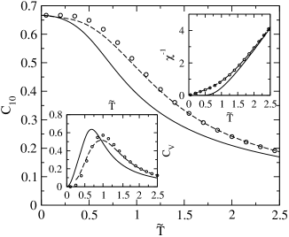
Figure 1: 2D $S=1$ ferromagnet: NN correlation function $C_{10}$, uniform static susceptibility $\chi$ (upper inset), and specific heat $C_{V}$ (lower inset) as functions of $\tilde{T}=T/[|J_{\parallel}|S(S+1)]$, where the results of the RGM in the thermodynamic limit (solid lines) and for $N=8$ (dashed lines) and the ED data ($\circ$, $N=8$) are shown.

Next, we consider the 2D antiferromagnet at finite temperatures. Since the case $S=1/2$ was intensively studied by the RGM in previous work,KY72 ; ISW99 we compare our results for $S=1$ with available QMC data.HTK98 As can be seen in Fig. 2, we obtain a surprisingly good agreement of the RGM with the QMC results (note that the QMC data for the correlation length agree with the SE results of Ref. ESS95, ). This agreement is much better than for the $S=1/2$ antiferromagnet.KY72 Correspondingly, for $S=1$ we can give a rather reliable value for the zero-temperature susceptibility, $\chi(0)=0.07197$.

As outlined in Sec. II, in our approach more vertex parameters are introduced as independent equations for

them can be provided by the RGM. Therefore, we have to formulate appropriate additional conditions for their determination. Let us discuss, in comparison to the choice fixed in Sec. II, two alternate choices of the parameters $\alpha_{2}$ and $\lambda$ for the 2D $S=1$ antiferromagnet (in two dimensions we omit the index $\mu=\parallel$, e.g., $\alpha_{1,2\parallel}=\alpha_{1,2}$), which are analogous to the choices made previously for the $S=1/2$ antiferromagnet,KY72 and the $S\geqslant 1$ ferromagnet.SSI94 (i) If we choose $\alpha_{2}=\alpha_{1}$, the parameter $\lambda(0)$ can be calculated (note that $\alpha_{2}$ and $\lambda$ only appear in the combination given by $\Delta$) and used in Eq. (18). Then, we find the finite-temperature results to be not in such a good agreement with the QMC data as the results obtained by the parameter choice with $\alpha_{2}\neq\alpha_{1}$. This corresponds to the findings for the $S=1/2$ antiferromagnetKY72 and may be understood as explained in Sec. II. Therefore, we discard the choice $\alpha_{2}=\alpha_{1}$. (ii) If we adopt $\alpha_{2}\neq\alpha_{1}$, but neglect the temperature dependence of $\lambda$, i.e., $\lambda(T)=\lambda(0)=2-\frac{1}{S}$ (as was assumed for the FM case in Ref. SSI94, ), the results appreciably deviate from the QMC data, as is demonstrated in Fig. 2 (dot-dashed lines). This gives strong arguments for taking into account the decrease of $\lambda(T)$ with increasing temperature [e.g., for $S=1$, we have $\lambda(0)=1$ and $\lambda_{\infty}=0.625$] and for our choice of the parameters for the antiferromagnet outlined on Sec. II. Note that for the $S=1$ ferromagnet, where $\alpha_{2}=\alpha_{1}$, the results shown in Fig. 1 only slightly improve those obtained by the assumption $\lambda(T)=\lambda(0)$.

Figure 2: 2D $S=1$ antiferromagnet: Correlation length $\xi$, uniform static susceptibility $\chi$ (upper inset), and staggered structure factor $C_{\bm{Q}}^{zz}=\frac{1}{2}C_{\bm{Q}}$ (lower inset) as functions of $\tilde{T}=T/[J_{\parallel}S(S+1)]$, where the RGM results (solid lines) are compared with the QMC data of Ref. HTK98, ($\bullet$). For comparison, the results of a simplified version of the RGM with $\lambda(T)=\lambda(0)$ (see text) are depicted (dot-dashed lines).

III.2 Transition temperatures

Table 2: Transition temperatures $\tilde{T}_{M}=T_{M}/[|J_{\parallel}|S(S+1)]$ of the ferromagnet ($\tilde{T}_{C}$) and antiferromagnet ($\tilde{T}_{N}$) calculated by the RGM for different spins $S$ and interlayer couplings $J_{\perp}/J_{\parallel}$.

	Ferromagnet			Antiferromagnet
n$J_{\bot}/J_{||}$nn	n $S=1/2$ n	n $S=1$ n	n $S=3/2$ n	n $S=1/2$ n	n $S=1$ n	n $S=3/2$ n	n $S=\infty$ n
0.0001	0.2457	0.3243	0.3542	0.1589	0.3393	0.3681	0.3305
0.0005	0.2928	0.3758	0.4041	0.2150	0.4014	0.4170	0.3785
0.001	0.3184	0.4027	0.4298	0.2498	0.4331	0.4421	0.4039
0.005	0.3961	0.4803	0.5035	0.3694	0.5195	0.5133	0.4784
0.01	0.4403	0.5226	0.5436	0.4430	0.5640	0.5521	0.5200
0.02	0.4935	0.5725	0.5911	0.5311	0.6150	0.5986	0.5698
0.05	0.5826	0.6552	0.6706	0.6681	0.6979	0.6776	0.6538
0.1	0.6699	0.7368	0.7503	0.7870	0.7800	0.7583	0.7378
0.5	0.9953	1.0571	1.0694	1.1655	1.1121	1.0884	1.0667
1.0	1.2346	1.3063	1.3208	1.4382	1.3762	1.3478	1.3189

An important problem in the study of layered ferromagnets and antiferromagnets is the calculation of the transition temperature $T_{M}$ ($M=C,N$) as a function of the interlayer coupling $J_{\perp}$ and of the spin quantum number $S$. From the experimental side, the knowledge of the dependence $T_{M}(R,S)$ with $R=J_{\perp}/J_{\parallel}$ is useful to estimate the interlayer exchange coupling from measurements of $T_{M}$. To test the quality of analytical approaches, the precise results of numerical methods, such as the QMCYTH05 and SE data,OZ04 should be used as benchmarks. Considering the 3D isotropic model ($R=1$), we have the inequalityOZ04 $T_{N}>T_{C}$. Moreover, $\tilde{T}_{M}\equiv T_{M}/[|J_{\parallel}|S(S+1)]$ is found to increase with increasing values of $S$.OZ04 ; YTH05 Considering, for example, the RPA, those results are not reproduced, instead we have $\tilde{T}_{N}^{\text{RPA}}=\tilde{T}_{C}^{\text{RPA}}$, where $\tilde{T}_{M}^{\text{RPA}}$ is independent of $S$.DW94 For layered magnets with $R<1$, QMC and SE data in the FM case are still missing, so that there are no precise statements about the relation between $T_{N}$ and $T_{C}$ as function of the interlayer coupling. With respect to the agreement with the QMC and SE data, our approach represents an important improvement as compared, e.g., to the RPA, which is outlined in the following.

Figure 3: Néel temperature $\tilde{T}_{N}=T_{N}/[J_{\parallel}S(S+1)]$ as a function of the interlayer coupling $R=J_{\perp}/{J_{\parallel}}$. The results of the RGM (solid lines) and of the empirical formula (20) (dashed lines) are compared with the QMC data ($\bullet$, Ref. YTH05, ), the RPA (dotted lines, Ref. DW94, ), and, for $S=1/2$ (inset), with the mean-field theories of Refs. IKK91, ($\square$), SI93, (dot-dashed line), and AA08, (dot-dot dashed line).

For the 3D ferro- and antiferromagnets, the solution of the RGM self-consistency equations yields the magnetization $m(T)$ with $m(T_{M})=0$ at the second-order phase transition temperature $T_{M}$, where $\lim_{J_{\perp}\to 0}T_{M}=0$ is in agreement with the Mermin-Wagner theorem.MW66 In Fig. 3 and Table 2 our results for $\tilde{T}_{M}$ as functions of $R$ and $S$ are presented, where in Fig. 3 the Néel temperature $\tilde{T}_{N}$ is compared with the QMC data of Ref. YTH05, and other approaches. For the $S=1$ antiferromagnet we get a very good agreement with the QMC results, as was also found for the 2D model (see Fig. 2). Remarkably, the RPA results for both the $S=1$ (Ref. DW94, ) and $S=1/2$ modelsDW94 ; MSS92 are in a rather good agreement with the QMC data. Considering the case $S=1/2$ (inset of Fig. 3) and $R<0.04$, we ascribe the reduction of $T_{N}$ found by the RGM as compared to the RPA and the mean-field approaches of Refs. IKK91, and SI93, to an improved description of strong AF quantum fluctuations at low temperatures counteracting the formation of LRO. For further comparison, the Néel temperature given very recentlyAA08 by the interlayer mean-field approach within the Schwinger-boson mean-field theory is depicted for $S=1/2$. The marked difference to the other curves (also found for $S=1$) might be due to the asymmetry between intralayer and interlayer correlations introduced in this approach.

Next we consider the transition temperatures $\tilde{T}_{M}$ for arbitrary values of $S$. The RGM yields $\tilde{T}_{C}(S)\neq\tilde{T}_{N}(S)$, as can be seen in Table 2, which is in accord with the QMC and SE data, but in contrast to the RPA result (see above). In passing to the classical limit $S\to\infty$ we find $\lim_{S\to\infty}\tilde{T}_{M}=\tilde{T}_{M}^{RPA}$ for all values of $R$. This may be understood as follows. The RGM is a second-order theory that goes one step beyond the RPA and, therefore, provides a better description of quantum fluctuations. Their vanishing for $S\to\infty$ may be reflected in the equality of the transition temperatures.

Table 3: Coefficients of the empirical law [Eq. (20)] for the transition temperatures of the ferro- and antiferromagnet.

	Ferromagnet			Antiferromagnet
	n $S=1/2$ n	n $S=1$ n	n $S=3/2$ n	n $S=1/2$ n	n $S=1$ n	n $S=3/2$ n	n $S=\infty$ n
$A$	3.15	4.00	4.27	1.95	4.36	4.34	3.96
$B$	2.50	3.08	3.27	0.01	3.21	3.27	3.01

We compare our results for the 3D isotropic model ($R=1$) with the SEOZ04 and QMC data YTH05 for different spins. For the ferromagnet, the Curie temperatures $\tilde{T}_{C}$ deviate from the SE values,OZ04 $\tilde{T}_{C}=1.119$ (1.2994, 1.37) for $S=\frac{1}{2}$, (1, $\frac{3}{2}$), by 10% (0.5%, 4%). For the antiferromagnet, the deviations of the Néel temperatures $\tilde{T}_{N}$ from the SE valuesOZ04 [agreeing with the QMC values for $S=1/2$ and $S=1$ (Ref. YTH05, )], $\tilde{T}_{N}=1.259$ (1.3676, 1.404) for $S=\frac{1}{2}$, (1, $\frac{3}{2}$), amount to 14%, (0.6%, 4%). From the experimental point of view, for the fit of exchange coupling parameters, deviations in the magnitude of transition temperatures of up to about 10% are considered as a reasonable accuracy. In both the FM and AF cases the RGM yields the best values of $\tilde{T}_{M}$ for $S=1$. For any spin, we get the correct relation $T_{N}>T_{C}$, where the ratio $Q=T_{N}/T_{C}=1.17$ (1.05, 1.02) for $S=\frac{1}{2}$, (1, $\frac{3}{2}$) agrees well with the SE values $Q=1.13$ (1.05, 1.03). That means, concerning the difference between $T_{N}$ and $T_{C}$, the RGM yields good results for all values of $S$. Considering the dependences $\tilde{T}_{M}(S)$, the increase of $\tilde{T}_{C}$ with increasing $S$ is in qualitative agreement with the SE data. For the antiferromagnet, $\tilde{T}_{N}$ decreases with increasing $S$ being opposite to the behavior of the SEOZ04 and QMC data.YTH05 This is connected with the inequality $\tilde{T}_{N}(S=\frac{1}{2})>\lim_{S\to\infty}\tilde{T}_{N}=1.3189$, whereas the QMC dataYTH05 ; HJ93 yield $\tilde{T}_{N}(S=\frac{1}{2})<\tilde{T}_{N}(S=\infty)=1.443$ [note that in the classical Heisenberg modelHJ93 the spins are taken of unit length, and the exchange interaction $J^{cl}$ is related to $J\equiv J_{\perp}=J_{\parallel}$ by $J^{cl}=JS(S+1)$].

Let us consider the anisotropic magnets ($R<1$). For $S=1/2$ and $R<0.01$ we find $T_{N}<T_{C}$, and for $R\geqslant 0.01$ we have $T_{N}>T_{C}$. In the cases $S=1$ and $S=3/2$ we get $T_{N}>T_{C}$ for all values of $R$. The peculiarity in the relation between $T_{N}$ and $T_{C}$ for $S=1/2$ may be explained by the presence of strong AF quantum fluctuations at low temperatures which may suppress the AF LRO.

For the discussion of experimental data it is convenient to use an analytical expression for $T_{M}(R,S)$. Our RGM results for the dependence of $\tilde{T}_{M}$ on $R$ may be well fitted by the empirical formula proposed in Ref. YTH05, ,

$$\tilde{T}_{M}=\frac{A}{B-\ln(J_{\perp}/J_{\parallel})},$$ (20)

where the values of $A$ and $B$ are listed in Table 3. The concrete values of the coefficients slightly depend on the choice of data points used for the fit. Since $T_{M}$ reveals the strongest increase with $R$ for $R\ll 1$, in this region we take points lying more dense than for moderate interlayer couplings. The values given in Table 3 are obtained by choosing points within the interval $R=10^{-4}$ to $10^{-2}$ and $R=10^{-2}$ to 1 in steps of $\Delta R=10^{-4}$ and $\Delta R=10^{-2}$, respectively. Then, a good fit in the whole $R$ region can be achieved in all cases, except for the $S=1/2$ antiferromagnet, where a reasonable fit by Eq. (20) is obtained for $R\leqslant 0.1$ (see Fig. 3).

III.3 Specific heat

Figure 4: Specific heat $C_{V}$ of the isotropic antiferromagnet ($J_{\perp}=J_{\parallel}$) with $S=1/2$, 1, 2, and 5, from bottom to top, in comparison to the QMC data for $S=1/2$ ($\bullet$, Ref. San98, ). The inset displays $C_{V}$ for the isotropic $S=1/2$ ferromagnet, compared to the SE results of Ref. OB96, ($\blacklozenge$).

Figure 5: Specific heat $C_{V}$ of the ferromagnet with $S=1/2$ and $S=1$ (inset) for $J_{\perp}/J_{\parallel}=0.01$ (solid lines), with $S=1/2$ for $J_{\perp}/J_{\parallel}=0.025$ (dot-dot dashed line) and 0.035 (dotted line), and with $S=1$ for $J_{\perp}/J_{\parallel}=0.015$ (dashed line) and 0.02 (dot-dashed line).

The temperature dependence of the specific heat $C_{V}$ is characterized by a cusplike singularity at the transition temperature $T_{M}$ determined by $J_{\perp}$ and, for sufficiently low interlayer couplings, by a broad maximum above $T_{M}$ that is mainly determined by $J_{\parallel}$. For the 3D isotropic magnets, $C_{V}$ is plotted in Fig. 4. Considering the $S=1/2$ ferromagnet (see inset), above $T_{C}$ we obtain an excellent agreement with the SE data of Ref. OB96, . For the $S=1/2$ antiferromagnet, the agreement of the RGM with the QMC resultsSan98 is very good at temperatures sufficiently below and above $T_{N}$, whereas near $T_{N}$ the height of the cusp is underestimated. Considering the $S$ dependence of $C_{V}$ in the LRO phase, with increasing $S$ the slope of the $C_{V}$ curves near $T_{N}$ decreases, and the cusp develops to a kink (see Fig. 4). The analogous tendency is found in the FM case. This behavior may be considered as a deficiency of the RGM, because in the classical Heisenberg model ($S\to\infty$) the QMC data of Ref. HJ94, yield evidence for a cusplike structure of $C_{V}$ at $T_{M}$.

Next we consider the specific heat of quasi-2D magnets. In the ferromagnet a broad maximum, in addition to the phase-transition singularity, appears at $R<0.035$ ($R\leqslant 0.015$) for $S=1/2$ ($S=1$), as can be seen in Fig. 5. The analogous behavior is found for the antiferromagnet, as shown in Fig. 6. Here, the broad maximum occurs at $R<2^{-3}$ ($R\leqslant 0.015$) for $S=1/2$ (S=1), which agrees with the $S=1/2$ QMC data of Ref. SSS03, . As for the isotropic $S=1/2$ antiferromagnet (cf. Fig. 4), the RGM agrees well with the QMC results at low and high temperatures. Again, the height of the cusp is underestimated, where the relative deviation of $C_{V}(T_{N})$ from the QMC values increases with decreasing $R$.

Figure 6: Specific heat of the $S=1/2$ antiferromagnet in comparison to the QMC data of Ref. SSS03, (filled symbols) for $J_{\perp}/J_{\parallel}=2^{-1}$ (solid line, $\bullet$), $2^{-2}$ (dashed line, $\blacktriangleright$), and $2^{-3}$ (dot-dashed line, $\blacklozenge$). The inset shows $C_{V}$ of the $S=1$ antiferromagnet for $J_{\perp}/J_{\parallel}=0.01$ (solid line), 0.015 (dashed line), and 0.02 (dot-dashed line).

Recently, specific heat data for the quasi-2D $S=1/2$ antiferromagnet Zn₂VO(PO₄)₂ were presented.KKG06 Taking $T_{N}=3.75$K and $J_{\parallel}=7.41$K from Ref. KKG06, , by Eq. (20) and Table 3 we get $R=5.8\times 10^{-2}$. Calculating the specific heat we obtain a broad maximum at $T_{m}=5.9$K with $C_{V}(T_{m})=0.45$ which corresponds to the measured broad hump at $T_{h}=4.5$K with the height $C_{V}(T_{h})=0.45$ agreeing with the theoretical value of $C_{V}(T_{m})$. At $T_{N}$, the experiment shows a pronounced cusp with $C_{V}(T_{N})\simeq 0.6$. As discussed above (see Fig. 6), this feature cannot be reproduced by the RGM, instead we get a small spike at $T_{N}$ with $C_{V}(T_{N})\simeq 0.3$.

III.4 Correlation length

Figure 7: Inverse correlation lengths within ($\xi_{\parallel}^{-1}$) and between the xy planes ($\xi_{\perp}^{-1}$, see inset) versus $\tilde{T}=T/[|J_{\parallel}|S(S+1)]$ of the ferromagnet with $S=1/2$ (solid lines) and $S=1$ (dashed lines) for $J_{\perp}/J_{\parallel}=0.001$, 0.1, and 1, from left to right.

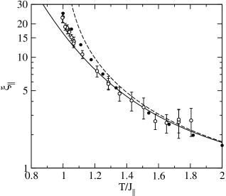
Figure 8: Antiferromagnetic intralayer correlation length in La₂NiO₄ obtained by the neutron-scattering experiments of Ref. NYH95, ($\circ$) compared to the QMC data for $J_{\perp}=0$ ($\bullet$, Ref. HTK98, ) and the RGM results for $J_{\perp}=0$ (solid line) and $J_{\perp}/J_{\parallel}=3.5\times 10^{-3}$ (dashed line).

The intralayer and interlayer correlation lengths $\xi_{\mu}$, ($\mu=\parallel,\perp$) for $R\neq 0$ diverge as $T$ approaches $T_{M}$ from above. In the vicinity of $T_{M}$, $\xi_{\parallel}^{-1}$ and $\xi_{\perp}^{-1}$ behave as $T-T_{M}$ (corresponding to the critical index $\nu=1$) also found by previous mean-field approaches.SI93 ; IKK99 This can be seen in Fig. 7 that shows $\xi_{\mu}^{-1}$ versus $\tilde{T}=T/[|J_{\parallel}|S(S+1)]$ of the $S=1/2$ and $S=1$ ferromagnet. The curves for the antiferromagnet look similar. At fixed $R<1$ and $S$ we have $\xi_{\perp}<\xi_{\parallel}$ which corresponds to the weaker interlayer as compared to the intralayer correlations. Considering the $S$ dependence of $\xi_{\mu}$ for the ferromagnet, we have $\tilde{T}_{C}(S=1/2)<\tilde{T}_{C}(S=1)$ (see Fig. 7 and Sec. III.2) which implies, at fixed $\tilde{T}>\tilde{T}_{C}$ and $R$, the inequality $\xi_{\mu}(S=1/2)<\xi_{\mu}(S=1)$. Note that recently, an analogous $S$ dependence for the lonitudinal correlation length $\xi^{zz}$ of the 2D ferromagnet in a small magnetic field was found, also by QMC,JIB08 i.e., $\xi^{zz}(S=1/2)<\xi^{zz}(S=1)$ at fixed $\tilde{T}$.

Let us compare our results for the intralayer correlation length $\xi_{\parallel}$ with the neutron-scattering data on the $S=1$ quasi-2D antiferromagnet La₂NiO₄.NYH95 Taking $T_{N}=327.5$K and $J_{\parallel}=28.7$meV from Ref. NYH95, , by Eq. (20) and Table 3 we obtain $R=3.5\times 10^{-3}$. In Fig. 8 the experimental data are plotted in comparison to the QMC data for $R=0$ (Ref. HTK98, ) and the RGM results for $R=0$ and $R=3.5\times 10^{-3}$, where a satisfactory overall agreement with experiments is found. At fixed temperature, the correlation length for $R>0$ is larger than for $R=0$, because $\xi_{\parallel}$ diverges at $T_{N}$. To explain the neutron-scattering experiments, in Ref. NYH95, a small Ising anisotropy in the strictly 2D model was considered which leads to in a finite transition temperature somewhat below $T_{N}$. Such an easy-axis anisotropy was also discussed in Ref. GP01, to explain the experiments. However, as was shown in Ref. HTK98, , the experimental data with $\xi^{\text{exp}}<\xi^{\text{QMC}}$ (see Fig. 8) are incompatible with the QMC results obtained for the 2D model with a small Ising anisotropy, since it even enhances the correlation length at low temperature. In our approach, the finite value of $T_{N}$ is ascribed entirely to the interlayer coupling which gives $\xi>\xi^{\text{QMC}}$. To improve the agreement with experiments, let us point out, that in our calculations a simple cubic lattice was taken, whereas in the orthorhombic structure of La₂NiO₄ the interlayer coupling is frustrated. As was shown in Ref. HRI08, , in the $J_{1}-J_{2}$ model, frustration may appreciably reduce the correlation length. The influence of frustration on the transition temperature and correlation length of quasi-2D Heisenberg magnets will be left for further study.

IV SUMMARY

In this paper the thermodynamics of layered Heisenberg magnets with arbitrary spin $S$ is systematically investigated by a spin-rotation-invariant Green-function method and by exact diagonalizations on finite 2D lattices. The main focus is put on the calculation of the Curie temperature $T_{C}$ and the Néel temperature $T_{N}$ in dependence on the interlayer coupling $J_{\perp}$ and the spin quantum number. From the numerical data we obtain simple empirical formulas for $T_{C,N}(J_{\perp})$. A good agreement of our results, in particular on the relation between $T_{C}$ and $T_{N}$, with available quantum Monte Carlo and series-expansion data is found. The comparison to experiments on the quasi-2D antiferromagnets Zn₂VO(PO₄)₂ and La₂NiO₄ yields a reasonable agreement. From our results we conclude that the application of the second-order Green-function approach to extended layered Heisenberg models (frustration, anisotropy in spin space) may be promising to describe the unconventional magnetic properties of real low-dimensional quantum spin systems.

References

- (1) Quantum Magnetism, Lecture Notes in Physics Vol. 645, edited by U. Schollwöck, J. Richter, D. J. J. Farnell, and R. F. Bishop (Springer, Berlin, 2004).
-
(2)
W-H. Li, C. H. Perry, J. B. Sokoloff, V. Wagner,
M. E. Chen, and G. Shirane, Phys. Rev. B 35, 1891 (1987);
S. Feldkemper, W. Weber, J. Schulenburg, and J. Richter,
ibid. 52, 313 (1995);
H. Manaka, T. Koide, T. Shidara, and I. Yamada, ibid. 68, 184412 (2003). - (3) K. Nakajima, K. Yamada, S. Hosoya, Y. Endoh, M. Greven, and R. J. Birgeneau, Z. Phys. B 96, 479 (1995).
- (4) L. Pisani, B. Montanari, and N. M. Harrison, New Journal of Physics 10, 033002 (2008).
- (5) P. Sengupta, A. W. Sandvik, and R. R. P. Singh, Phys. Rev. B 68, 094423 (2003).
- (6) C. Yasuda, S. Todo, K. Hukushima, F. Alet, M. Keller, M. Troyer, and H. Takayama, Phys. Rev. Lett. 94, 217201 (2005).
- (7) A. W. Sandvik, Phys. Rev. Lett. 80, 5196 (1998).
- (8) J. Oitmaa and W. Zheng, J. Phys.:Condens. Matter 16, 8653 (2004).
- (9) J. Oitmaa and E. Bornilla, Phys. Rev. B 53, 14228 (1996).
- (10) N. Majlis, S. Selzer, and G. C. Strinati, Phys. Rev. B 45, 7872 (1992).
- (11) A. Du and G. Z. Wei, J. Magn. Magn. Mat. 137, 343 (1994).
- (12) S. V. Tyablikov, Methods in the Quantum Theory of Magnetism (Plenum, New York, 1967).
- (13) V. Yu. Irkhin, A. A. Katanin, and M. I. Katsnelson, Phys. Lett. A 157, 295 (1991).
- (14) A. Auerbach and D. P. Arovas, arXiv:0809.4836v2 [cond-mat. str-el].
- (15) F. Suzuki and C. Ishii, J. Phys. Soc. Jpn. 62, 3686 (1993).
- (16) V. Yu. Irkhin, A. A. Katanin, and M. I. Katsnelson, Phys. Rev. B 60, 1082 (1999).
- (17) P. Gianinetti and A. Parola, Phys. Rev. B 63, 104414 (2001).
- (18) J. Kondo and K. Yamaji, Prog. Theor. Phys. 47, 807 (1972); H. Shimahara and S. Takada, J. Phys. Soc. Jpn. 60, 2394 (1991); S. Winterfeldt and D. Ihle, Phys. Rev. B 56, 5535 (1997).
- (19) F. Suzuki, N. Shibata, and C. Ishii, J. Phys. Soc. Jpn. 63, 1539 (1994).
- (20) D. Ihle, C. Schindelin, A. Weiße, and H. Fehske, Phys. Rev. B 60, 9240 (1999); D. Ihle, C. Schindelin, and H. Fehske, Phys. Rev. B 64, 054419 (2001).
- (21) W. Yu and S. Feng, Eur. Phys. J. B 13, 265 (2000); B. H. Bernhard, B. Canals, and C. Lacroix, Phys. Rev. B 66, 104424 (2002).
- (22) L. Siurakshina, D. Ihle, and R. Hayn, Phys. Rev. B 61, 14601 (2000).
- (23) I. Junger, D. Ihle, J. Richter, and A. Klümper, Phys. Rev. B 70, 104419 (2004).
- (24) T. N. Antsygina, M. I. Poltavskaya, I. I. Poltavsky, and K. A. Chishko, Phys. Rev. B 77, 024407 (2008).
- (25) I. Juhász Junger, D. Ihle, L. Bogacz, and W. Janke, Phys. Rev. B 77, 174411 (2008).
- (26) D. Schmalfuß, J. Richter, and D. Ihle, Phys. Rev. B 70, 184412 (2004); D. Schmalfuß, R. Darradi, J. Richter, J. Schulenburg, and D. Ihle, Phs. Rev. Lett. 97, 157201 (2006).
- (27) I. Juhász Junger, D. Ihle, and J. Richter, Phys. Rev. B 72, 064454 (2005).
- (28) D. Schmalfuß, J. Richter, and D. Ihle, Phys. Rev. B 72, 224405 (2005).
- (29) M. Härtel, J. Richter, D. Ihle, and S.-L. Drechsler, Phys. Rev. B 78, 174412 (2008).
- (30) A. V. Mikheyenkov, N. A. Kozlov, and A. F. Barabanov, Phys. Lett. A 373, 693 (2009).
- (31) W. H. Press, S. A. Teukolsky, W. T. Vetterling and B. P. Flannery, Numerical Recipes in Fortran 77: The Art of Scientific Computing (Cambridge University Press, Cambridge, 2001).
- (32) K. Harada, M. Troyer, and N. Kawashima, J. Phys. Soc. Jpn. 67, 1130 (1998).
- (33) N. Elstner, A. Sokol, R. R. P. Singh, M. Greven, and R. J. Birgeneau, Phys. Rev. Lett. 75, 938 (1995).
- (34) N. Mermin and H. Wagner, Phys. Rev. Lett. 17, 1133 (1966).
- (35) C. Holm and W. Janke, Phys. Rev. B 48, 936 (1993); K. Chen, A. M. Ferrenberg, and D. P. Landau, Phys. Rev. B 48, 3249 (1993).
- (36) C. Holm and W. Janke, J. Phys. A: Math. Gen. 27, 2553 (1994).
- (37) N. S. Kini, E. E. Kaul, and C. Geibel, J. Phys.: Condens. Matter 18, 1303 (2006).