Kondo effect and conductance of nanocontacts with magnetic impurities

Abstract

We study the impact of dynamical correlations on the electronic structure and coherent transport properties of Cu nanocontacts hosting a single magnetic impurity (Ni,Co,Fe) in the contact region. The strong dynamical correlations of the impurity $3d$-electrons are fully taken into account by combining density functional calculations with a dynamical treatment of the impurity $3d$-shell in the one-crossing approximation. We find that dynamical correlations give rise to the Kondo effect and lead to Fano features in the coherent transport characteristics similar to those observed in related experiments.

The development of nanoscale spintronics devices based on single molecules and atomic size junctions containing magnetic atoms is a fascinating and challenging field of research at the moment Tsukagoshi-Zhao-Hueso-Bogani . An important contribution to the electronic structure and transport properties of these devices comes from the strongly interacting $d$- or $f$-electrons of the magnetic atoms. The strong interactions result in dynamical correlations that give rise to interesting effects like e.g. the Kondo effect. For example, Fano lineshapes Fano (1961) observed in the conductance characteristics of scanning tunneling microscope (STM) experiments with magnetic adatoms and molecular complexes on metal surfaces Madhavan-Vitali-Neel ; Néel et al. (2007) are the result of Kondo resonances at the Fermi level Kondo (1964); Schiller and Hershfield (2000). Recently, Fano lineshapes have also been observed in the non-linear conductance characteristics of chemically homogeneous nanocontacts Agraït et al. (2003) made from ferromagnetic transition metals (Ni, Co, Fe) Calvo et al. (2009).

State of the art calculations of the conductance and current through atomic- and molecular-size conductors consist in combining ab initio electronic structure calculations on the level of density-functional theory (DFT) with the non-equilibrium Green’s function (NEGF) technique abinitnegf . This methodology works quite well for metallic nanocontacts Agraït et al. (2003) predicting zero-bias conductances that are in general in good agreement with experiments nanocontacts . However, static mean-field methods like DFT cannot describe dynamical electron correlations. Thus the DFT based ab initio transport methodology is not capable of describing the Fano-Kondo lineshapes Fano (1961) observed in STM studies of magnetic adatoms on surfaces Madhavan-Vitali-Neel ; Néel et al. (2007).

In order to explore the impact of strong dynamic correlations on the transport properties of atomic- and molecular-size conductors, we study Cu nanocontacts hosting magnetic impurities in the contact region. Such a system could also be realized experimentally with e.g. the break junction technique Agraït et al. (2003) using alloys containing magnetic atoms like e.g. Cupronickel. To this end we extend the established DFT based ab initio quantum transport methodology to incorporate dynamic electron correlations by adapting the LDA+DMFT method Kotliar et al. (2006) to the case of a single magnetic impurity in a nanocontact. While the strong dynamic correlations of the impurity $d$-electrons are fully taken into account, the rest of the system is described on a static mean-field level in the local density approximation (LDA) to DFT. Other recent approaches to include dynamic electron correlations in the ab initio description of quantum transport are based on the GW approximation (GWA) Thygesen and Rubio (2007) or the three-body scattering formalism (3BS) Ferretti et al. (2005). While the GWA is only suitable for weakly correlated systems due to the perturbative treatment of the electron-electron interactions, the 3BS is in principle capable of describing more strongly correlated systems as it goes beyond perturbation theory. However, the 3BS does not provide a satisfactory solution of the Anderson impurity problem since the local correlations are not taken into account properly. In contrast, in our method both the strong Coulomb interactions between the impurity $d$-electrons and the resulting local correlations are taken into account properly.

We consider a single magnetic impurity bridging the tips of two semi-infinite Cu nanowires of finite width grown in the (001) direction as shown in Fig. 1. We divide the system into three parts as shown in the right panel of Fig. 1: Two semi-infnite leads L and R, and the central device region (D) which contains the central magnetic impurity with the strongly interacting $3d$-shell ($d$), and the tips of the two electrodes. The device also contains a sufficient part of the semi-infinite leads so that the two leads L and R are sufficiently far away from the scattering region and the electronic structure of the leads has relaxed to that of bulk (i.e. infinite) nanowires. The effective one-body Hamiltonians of the device region and leads are obtained from DFT calculations on the level of LDA. Here we use the supercell approach foo to obtain the effective Kohn-Sham (KS) Hamiltonians of each part of the system prior to the dynamical treatment of the impurity $d$-shell and the transport calculations. The electronic structure of the device region is calculated with the CRYSTAL06 ab initio electronic structure program for periodic systems Dovesi et al. by definining a one-dimensional periodic system consisting of the device region as the unit cell. The device Hamiltonian $\mathbf{H}_{D}$ is then obtained from the converged KS Hamiltonian of the unit cell of the periodic system. In the same way, the unit cell Hamiltonians $\mathbf{H}^{0}_{\rm L/R}$ and hoppings $\mathbf{V}_{\rm L/R}$ between unit cells of the left and right leads can be extracted from calulcations of infinite nanowires with finite width since the electronic structure in the semi-infinite leads has relaxed to that of an infinite nanowire. In the LDA calculations we employ a minimal basis set plus effective core pseudo-potential that takes into account only the $4s$, $4p$ and $3d$ valence shells of the Cu atoms and the magnetic impurity Hurley et al. (1986).

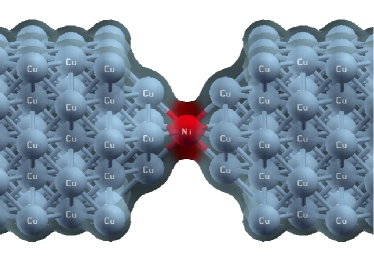
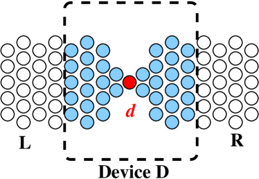
Figure 1: (Color online) Left: Atomic model of a Cu nanocontact with a magnetic impurity (red) in the contact region. Right: Division of system into left (L) and right (R) electrode, and central device region (D) containing the magnetic impurity (red) hosting the strongly correlated $d$-orbitals.

The strong electron correlations in the $3d$-shell of the magnetic impurity are captured by adding a Hubbard-like interaction term to the one-body Hamiltonian within the correlated subspace $d$: $\hat{\mathcal{H}}_{U}=\frac{1}{2}\sum U_{ijkl}\,\hat{c}_{i\sigma_{1}}^{\dagger}\hat{c}_{j\sigma_{2}}^{\dagger}\hat{c}_{l\sigma_{2}}\hat{c}_{k\sigma_{1}}$ (Einstein sum convention). $U_{ijkl}$ are the matrix elements of the effective Coulomb interaction of the $3d$-electrons which is smaller than the bare Coulomb interaction due to the screening by the conduction electrons. In the spherical approximation all matrix elements $U_{ijkl}$ can be calculated from the Slater integrals $F^{0}$, $F^{2}$, and $F^{4}$ which are related to the average Coulomb repulsion $U$ between electrons and to the Hund’s rule coupling $J$ by $F^{0}=U$, $F^{2}=(14/1.625)J$, and $F^{4}=0.625F^{4}$ Kotliar et al. (2006). For $3d$ transition metal elements in bulk materials the repulsion $U$ is around 2-3 eV and $J$ is around 1 eV Grechnev et al. (2007). Due to the lower coordination of the contact atoms the screening of the direct interaction is reduced compared to its bulk value. Here we take $U=5$ eV and $J=1$ eV, but we have checked that the results do not change much when $U$ is varied between 4 and 6 eV.

The Coulomb interaction within the correlated $3d$ subspace has already been taken into account on a static mean-field level in the effective KS Hamiltonian of the device. Therefore the KS Hamiltonian within the correlated subspace $\mathbf{H}_{d}$ has to be corrected by a double-counting correction term, i.e. $\mathbf{H}_{d}\equiv\mathbf{H}_{d}^{\rm KS}-\mathbf{H}_{\rm dc}$. Here we use the standard expression, $\mathbf{H}_{\rm dc}=[U(N_{d}-\frac{1}{2})-\frac{1}{2}J(N_{d}-1)]\times\mathbf{I}_{d}$ where $\mathbf{I}_{d}$ is the identity matrix in the $d$ subspace, and $N_{d}$ is the occupation of the impurity $3d$-shell Kotliar et al. (2006).

The central quantity is the Green’s function (GF) of the device region:

$$\mathbf{G}_{\rm D}=\left(\omega+\mu-\mathbf{H}_{\rm D}+\mathbf{H}_{\rm dc}-\mathbf{\Sigma}_{d}-\mathbf{\Sigma}_{\rm L}-\mathbf{\Sigma}_{\rm R}\right)^{-1}$$ (1)

where $\mu$ is the chemical potential. $\mathbf{\Sigma}_{\rm L}$ and $\mathbf{\Sigma}_{\rm R}$ are self-energies that describe the coupling of the device to the semi-infinite leads L and R, respectively. These can be calculated from the effective one-body Hamiltonians of the leads by iteratively solving the Dyson equation $\mathbf{\Sigma}_{\rm L/R}=\mathbf{V}_{\rm L/R}(\omega+\mu-\mathbf{H}^{0}_{\rm L/R}-\mathbf{\Sigma}_{\rm L/R})^{-1}\mathbf{V}_{\rm L/R}^{\dagger}$. $\mathbf{\Sigma}_{d}$ is the local electronic self-energy that describes the dynamic electron correlations of the impurity $3d$-electrons. In order to calculate $\mathbf{\Sigma}_{d}$, the generalized Anderson impurity problem given by the impurity $3d$-shell has to be solved. The impurity problem is described by the projection $\mathbf{P}_{d}$ of the GF (1) onto the correlated subspace $d$: $\mathbf{G}_{d}\equiv\mathbf{P}_{d}\mathbf{G}_{\rm D}\mathbf{P}_{d}$ which can be written as

$$\mathbf{G}_{d}(\omega)=\left(\omega+\mu-\mathbf{H}_{d}-\mathbf{\Sigma}_{d}(\omega)-\mathbf{\Delta}_{d}(\omega)\right)^{-1}$$ (2)

where we have introduced the so-called hybridization function $\mathbf{\Delta}_{d}$ which describes the hybridization of the impurity electrons with the conduction electrons. The hybridization function can be calculated from the projection $\mathbf{P}_{d}$ of the uncorrelated device GF $\mathbf{G}_{D}^{0}=\left(\omega+\mu-\mathbf{H}_{D}+\mathbf{H}_{dc}-\mathbf{\Sigma}_{L}-\mathbf{\Sigma}_{R}\right)^{-1}$ onto the correlated subspace $d$ foo , i.e. from $\mathbf{G}_{d}^{0}\equiv\mathbf{P}_{d}\mathbf{G}_{D}^{0}\mathbf{P}_{d}$. Solving eq. (2) for $\mathbf{\Delta}_{d}$ and using that $[\mathbf{G}_{d}]^{-1}=[\mathbf{G}_{d}^{0}]^{-1}-\mathbf{\Sigma}_{d}$ we obtain:

$$\mathbf{\Delta}_{d}(\omega)=\omega+\mu-\mathbf{H}_{d}-[\mathbf{G}_{d}^{0}(\omega)]^{-1}$$ (3)

The hybridization function $\mathbf{\Delta}_{d}$ foo , the Coulomb repulsion $U$, the Hund’s rule coupling $J$, and the impurity levels $\epsilon_{d,i}=(\mathbf{H}_{d})_{ii}$ are the relevant parameters for solving the impurity problem. Here we employ the so-called One-Crossing-Approximation (OCA) to solve the impurity problem Haule et al. (2001); Kotliar et al. (2006) which is particularly well suited for the Kondo regime.

The current through a strongly interacting impurity can be calculated exactly by the Meir-Wingreen formula Meir and Wingreen (1992). However, for low temperatures and small bias voltages this expression is well approximated by the much simpler Landauer formula Landauer (1970): $I(V)=\frac{2e}{h}\times\int_{0}^{eV}d\omega\,T(\omega)$ where $T(\omega)$ is the Landauer transmission function and where we have assumed an asymmetric voltage drop $V$ about the device region foo . Thus the conductance is simply given by the Landauer transmission function: $\mathcal{G}(V)=\frac{\partial I}{\partial V}(V)=\frac{2e^{2}}{h}\times T(eV)$. The latter can be calculated from the device Green’s function: $T(\omega)={\rm Tr}[\mathbf{\Gamma}_{L}(\omega)\mathbf{G}_{D}^{\dagger}(\omega)\mathbf{\Gamma}_{R}(\omega)\mathbf{G}_{D}(\omega)]$ where $\mathbf{\Gamma}_{L/R}$ are the so-called coupling matrices which describe the coupling to the leads, and can be calculated from the lead self-energies by $\mathbf{\Gamma}_{L/R}=i(\mathbf{\Sigma}_{L/R}-\mathbf{\Sigma}^{\dagger}_{L/R})$.

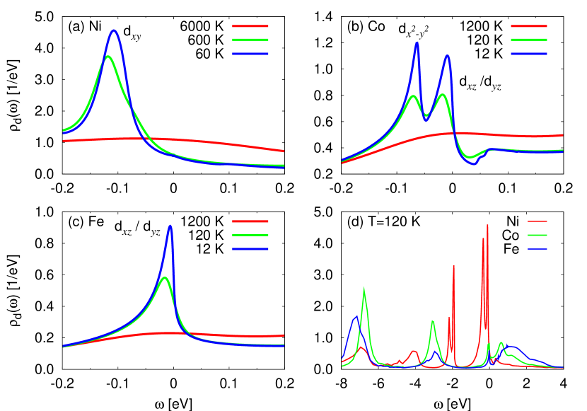
Figure 2: (Color online) PDOS of $d$-orbitals calculated with the LDA+OCA method for different magnetic impurities in Cu nanocontact for the geometry shown in Fig. 1. (a)-(c) PDOS near Fermi level for a Ni (a), Co (b) and Fe (c) impurity at different temperatures. (d) Comparison of the PDOS of the three impurities on a larger energy scale at $T=120$ K. $U=5$ eV and $J=1$ eV in all cases.

Fig. 2 shows the result of our LDA+OCA calculations for three different impurities: Ni, Co, and Fe, for different temperatures. In all three cases the partial density of states (PDOS) for the impurity $3d$-electrons shows resonances near the Fermi level which are temperature-dependent. More precisely, the resonances vanish with increasing temperature. This is characteristic for the Kondo effect which is usually observed only at low temperature. The resonances originate from different $d$-orbitals in each case, as indicated by the labels in the figures. In the case of Ni, the resonance originates from the $d_{xy}$-orbital. In the case of Co, there are two distinct peaks corresponding to two different sets of orbitals: The peak that is farther from (closer to) the Fermi level originates from the $d_{x^{2}-y^{2}}$ ($d_{xz},d_{yz}$) orbital(s). The doubly-degenerate $d_{xz},d_{yz}$-orbitals are also responsible for the resonance in the case of Fe. As can be seen from Figs. 3(a)-(c) the corresponding conductances all show Fano-like features. Interestingly, in the case of Co, the $d_{x^{2}-y^{2}}$-resonance does not lead to a corresponding feature in the conductance characteristics. This can be understood by the so-called orbital blocking: The electron transport through certain orbitals can be inhibited by the geometry or symmetry of atomic-size conductors in spite of the orbital having spectral weight near the Fermi energy Jacob et al. (2005).

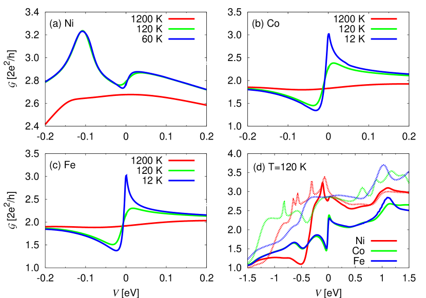
Figure 3: (Color online) Conductance calculated with LDA+OCA method for different magnetic impurities in Cu nanocontact for the geometry shown in Fig. 1: (a)-(c) Conductance $\mathcal{G}$ vs. bias voltage $V$ for different temperatures and for small bias. (d) Comparison of LDA+OCA (solid lines) and LSDA (dashed lines) conductances for different impurities at $T=120$ K. $U=5$ eV and $J=1$ eV in all cases.

Tab. 1 shows the orbital occupations and effective energy levels $\tilde{\epsilon}_{d}\equiv\epsilon_{d}+{\rm Re}\;\Delta_{d}(0)$ of the impurity $3d$-shell for different impurity atoms. One can see, that the effective energy levels $\tilde{\epsilon}_{d}$ roughly correlate with the orbital occupations except in the case of the $d_{x^{2}-y^{2}}$-orbital in Ni and Fe. To fully understand the orbital occupations, the imaginary part of the hybridization function $\Delta_{d}$ has to be taken into account. The imaginary part of $\Delta_{d}$ describes the broadening of the $d$-orbitals due to the coupling to the conduction electrons. It turns out that the $d_{x^{2}-y^{2}}$-orbital is by far the most localized orbital of all the $d$-orbitals i.e. the broadening is very small compared to the other $d$-levels foo . This explains why the $d_{x^{2}-y^{2}}$-orbital in Ni and Fe is only half-filled despite its low effective energy $\tilde{\epsilon}_{d}$.

Furthermore, we see that for Ni the $d_{xy}$-orbital which gives rise to the resonance near the Fermi energy is almost completely filled. Hence it does not carry a spin-1/2 and therefore the system is not in the Kondo regime, but is in the so-called empty orbital regime Hewson (1993). A broad quasiparticle (QP) peak quite close to the Fermi level appears which —as in the Kondo regime— arises from the Fermi liquid behaviour at low temperatures. The temperature dependence of the QP peak is qualitatively similar to the Kondo regime, i.e. the peak broadens with increasing temperature and disappears above a critical temperature, called the Kondo temperature $T_{\rm K}$. For the Co and the Fe impurity, the doubly-degenerate orbitals $d_{xz}$ and $d_{yz}$ that give rise to the QP resonance at the Fermi level are occupied by three electrons (filling 3/4) and thus carry a spin-1/2. Therefore in the case of Co and Fe, the system really is in the Kondo regime.

We have estimated the Kondo temperatures $T_{\rm K}$ displayed in Tab. 1 from the width of the QP peaks at low temperature. The Kondo temperatures follow the same trend, namely $T_{\rm K}({\rm Ni})>T_{\rm K}({\rm Co})>T_{\rm K}({\rm Fe})$, which is also observed in STM experiments with adatoms on metal surfaces Jamneala et al. (2000) and in pure transition metal nanocontacts Calvo et al. (2009). Moreover, the Kondo temperature for Co agrees quite well with the $T_{K}$ estimated from recent STM experiments with Co adatoms on Cu surfaces in the contact regime Néel et al. (2007). The high Kondo temperatures of about 200 K for Co and Fe imply a strong antiferromagnetic coupling $J_{sd}$ between the conduction electrons and the impurity $d$-electrons giving rise to the Kondo effect since $T_{\rm K}\propto\exp(-1/J_{sd}\rho_{0})$ where $\rho_{0}$ is the conduction electron DOS at the Fermi level Hewson (1993). This strong antiferromagnetic coupling might explain why the Kondo effect is observed in ferromagnetic nanocontacts despite the ferromagnetic coupling to the bulk electrodes Calvo et al. (2009).

Imp.:	Ni		Co		Fe
	$n_{d}$	$\tilde{\epsilon}_{d}$ [eV]	$n_{d}$	$\tilde{\epsilon}_{d}$ [eV]	$n_{d}$	$\tilde{\epsilon}_{d}$ [eV]
$d_{3z^{2}-r^{2}}$	1.92	0	1.01	0	1.00	0
$d_{xz},d_{yz}$	3.60	-0.22	3.05	-0.35	3.02	-0.71
$d_{x^{2}-y^{2}}$	1.00	-0.05	1.98	-0.35	1.00	-0.43
$d_{xy}$	1.90	-0.26	1.00	-0.03	1.00	-0.24
$N_{d}$	8.42		7.04		6.02
$T_{\rm K}$ [K]	$\sim$ 500		$\sim$ 225		$\sim$ 160

Table 1: Orbital occupations $n_{d}$, effective energy levels $\tilde{\epsilon}_{d}=\epsilon_{d}+{\rm Re}\;\Delta_{d}(0)$ of impurity $d$-levels relative to $d_{3z^{2}-r^{2}}$-level, total occupation $N_{d}$ of the impurity $3d$-shell and Kondo temperature $T_{\rm K}$ estimated from the width of the resonance closest to the Fermi level for each of the three impurities. $U=5$ eV, $J=1$ eV.

Finally, in Fig. 3(d) we compare the results obtained with the LDA+OCA method at low temperature with results obtained from DFT calculations on the level of the local spin density approximation (LSDA). For Ni (red lines) the effect of including dynamic correlations is only moderate. Thus for Ni the static mean-field description given by LSDA is a reasonable approximation to the fully correlated description by the LDA+OCA method, but at the cost of breaking the spin symmetry. This can be understood by recognizing that LSDA usually gives reasonable spectra for the empty orbital and mixed valence regimes. In contrast for Co (green lines) and Fe (blue lines) taking into account dynamical correlations changes the conductance substantially. The dynamic correlations open a gap in the $3d$-shell thereby taking away spectral weight from the Fermi level, leaving only the Kondo resonance (with small spectral weight) at low temperatures. Consequently, the conductances predicted by LDA+OCA are considerably lower than the conductances predicted by LDA and LSDA.

In conclusion, we have extended the established DFT based ab initio transport methodology for nanoscopic conductors to include dynamic electron correlations. We find that nanocontacts hosting a magnetic impurity show strong dynamical correlations which give rise to quasiparticle resonances at the Fermi level and corresponding Fano features in the conductance-voltage characteristics. Our findings agree well with experiments measuring the conductance through Co adatoms on metal surfaces in the contact regime. Moreover, our results shed some light on the recent observation of the Kondo effect in ferromagnetic nanocontacts.

DJ acknowledges funding by the German academic exchange service (DAAD) and fruitful discussions with J. J. Palacios, J. Fernández-Rossier, C. Untiedt and R. Calvo. KH was supported by the NSF under grant No. DMR 0746395 and by a Sloan fellowship. GK acknowledges funding by NSF under grant No. DMR 0528969.

References

- (1) K. Tsukagoshi, B. W. Alpenhaar, and H. Ago, Nature 401, 572 (1999); A. Zhao et al., Science 309, 1542 (2005); L. E. Hueso et al., Nature 445, 410 (2007); L. Bogani and W. Wernsdorfer, Nature Materials 7, 179 (2008).
- Fano (1961) U. Fano, Phys. Rev. 124, 1866 (1961).
- (3) V. Madhavan et al., Science 280, 567 (1998); L. Vitali et al., Phys. Rev. Lett. 101, 216802 (2008); N. Neél et al., Phys. Rev. Lett. 101, 266803 (2008).
- Néel et al. (2007) N. Néel et al., Phys. Rev. Lett. 98, 016801 (2007).
- Kondo (1964) J. Kondo, Prog. Theor. Phys. 32, 37 (1964).
- Schiller and Hershfield (2000) A. Schiller and S. Hershfield, Phys. Rev. B 61, 9036 (2000).
- Agraït et al. (2003) N. Agraït, A. L. Yeyati, and J. M. van Ruitenbeek, Physics Reports 377, 81 (2003), and references therein.
- Calvo et al. (2009) M. R. Calvo et al., Nature 358, 1150 (2009).
- (9) J. Taylor, H. Guo, and J. Wang, Phys. Rev. B 63, 245407 (2001); J. J. Palacios et al., Phys. Rev. B 64, 115411 (2001).
- Jacob et al. (2005) D. Jacob, J. Fernández-Rossier, and J. J. Palacios, Phys. Rev. B 71, 220403(R) (2005).
- (11) C. Untiedt et al., Phys. Rev. B 66, 085418 (2002); M. Viret et al., Phys. Rev. B 66, 220401(R) (2002); Z. K. Keane, L. H. Yu, and D. Natelson, Appl. Phys. Lett. 88, 062514 (2006); K. I. Bolotin et al., Nano Lett. 6, 123 (2006).
- Smogunov et al. (2006) A. Smogunov, A. DalCorso, and E. Tosatti, Phys. Rev. B 73, 075418 (2006).
- Kotliar et al. (2006) G. Kotliar et al., Rev. Mod. Phys. 78, 865 (2006).
- Thygesen and Rubio (2007) K. S. Thygesen and A. Rubio, J . Chem. Phys. 126, 091101 (2007).
- Ferretti et al. (2005) A. Ferretti et al., Phys. Rev. Lett. 94, 116802 (2005).
- (16) See EPAPS No. XXXX for details of the supercell approach, a detailed derivation of eq. (3), and a display of the hybridization function.
- (17) R. Dovesi et al., CRYSTAL06, Release 1.0.2, Theoretical Chemistry Group - Universita’ Di Torino - Torino (Italy).
- Hurley et al. (1986) M. M. Hurley et al., J. Chem. Phys 84, 6840 (1986).
- Grechnev et al. (2007) A. Grechnev et al., Phys. Rev. B 76, 035107 (2007).
- Haule et al. (2001) K. Haule et al., Phys. Rev. B 64, 155111 (2001).
- Meir and Wingreen (1992) Y. Meir and N. S. Wingreen, Phys. Rev. Lett. 68, 2512 (1992).
- Landauer (1970) R. Landauer, Philos. Mag. 21, 863 (1970).
- (23) For the idealized contact geometry considered here, the voltage drop would actually be symmetric. However, in reality the geometries are often quite asymmetric so that our assumption is justified.
- Hewson (1993) A. C. Hewson, The Kondo problem to heavy fermions (Cambridge University Press, 1993).
- Jamneala et al. (2000) T. Jamneala et al., Phys. Rev. B 61, 9990 (2000).