Vibrated granular gas confined by a piston

Abstract

The steady state of a vibrated granular gas confined by a movable piston on the top is discussed. Particular attention is given to the hydrodynamic boundary conditions to be used when solving the inelastic Navier-Stokes equations. The relevance of an exact general condition relating the grain fluxes approaching and moving away from each of the walls is emphasized. It is shown how it can be used to get a consistent hydrodynamic description of the boundaries. The obtained expressions for the fields do not contain any undetermined parameter. Comparison of the theoretical predictions with molecular dynamics simulation results is carried out, and a good agreement is observed for low density and not too large inelasticity. A practical way of introducing small finite density corrections to the dilute limit theory is proposed, to improve the accuracy of the theory.

I Introduction

The behavior of fluidized granular systems resembles in many cases that of ordinary molecular fluids. Actually, it is by now well established that generalized Navier-Stokes equations describe quite accurately many of the experimental and numerical features of granular flows, especially at low density and small inelasticity Ha83 ; Ca90 ; Go03 . The justification for this fluid-like description, and derivation of theoretical predictions for the transport coefficients appearing in the equations, have been intensively studied for some time. Quite often, idealized systems of inelastic hard spheres or disks have been considered. For mono-disperse models of this kind, the studies carried out include the derivation of the hydrodynamic equations to Navier-Stokes order by using kinetic theory methods LSJyCh84 ; JyR85 ; SyG98 ; BDKyS98 ; GyD99 ; ByD05 , direct Monte Carlo simulation of (inelastic) kinetic equations BRyC96 ; ByC01 , molecular dynamics simulations He95 , and, very recently, linear response theory DByB08 ; BDyB08 .

Interactions between grains are inherently inelastic. As a consequence, the kinetic energy of isolated granular systems decreases monotonically in time and, in order to keep them fluidized, it is necessary to continuously supply energy to them. A prototypical way of doing it is by vibrating one of the walls of the container, usually the one at the bottom. Also often, the interest focuses on the bulk properties of the system, i.e. on the behavior of the system far enough from the walls, where the governing laws are expected to be independent of the details of the boundaries. Then, the most appropriate possible way of vibration for this purpose is chosen. In many situations of interest, the criterium for this choice is twofold: simplicity and avoiding undesired effects such as the induction of propagating waves into the system. These goals are formally achieved in the limits of very high frequency and very small amplitude; the former as compared with the typical relaxation frequency of the granular fluid next to the wall, and the latter with its mean free path. Additional simplifications occur if collisions of the grains with the wall are taken as elastic and if the wall is assumed to move with a sawtooth profile McyB97 ; McyL98 .

A kind of idealized walls often used in kinetic theory and particle simulations are the so-called thermal walls. By definition, the flux of after-collision particles leaving it corresponds to a Maxwellian flux with the temperature parameter characterizing the wall DyvB57 . Therefore, the shape of the velocity distribution of the particles moving away from the thermal wall is independent of the distribution of the ingoing particles. It is evident that thermal walls also provide a mechanism to compensate the energy dissipated in inelastic collisions, once the granular gas in the vicinity of the wall tends to have a temperature smaller than the one of the wall. It is then not surprising that thermal walls have also been extensively used in the literature of fluidized granular gases since a decade ago GZyB97 ; ByC98 . Nevertheless, it must be stressed that it is not at all evident that thermal walls correspond to any limit of a rapidly vibrating plate. Actually, it has been shown that in some cases the stability of systems driven by a thermal wall and by a wall vibrating in a sawtooth way can differ BRMyG02 .

The granular system considered in this paper is confined between two parallel plates in presence of a gravity force. The mission of the one at the bottom of the system is to fluidize the granular medium, as in the previous studies mentioned above. On the other hand, the wall on the top is floating, in the sense that it can move in the vertical direction, being supported by the granular fluid below it. As a consequence, the position and motion of the upper wall is interrelated with the state of the granular media below it, and the boundary conditions to be imposed to the hydrodynamic equations, following from the interaction between the gas and the piston, must be determined in a self-consistent way. Here, the steady state eventually reached by the granular gas between the two plates will be investigated, using the hydrodynamic description provided by the Navier-Stokes equations for inelastic hard spheres. Collisions of the grains with the piston will be modeled as hard inelastic collisions. This defines in a deterministic way the mechanical interaction between the particles and the movable wall. The question addressed afterwards is how to translate it into an appropriate boundary condition to be used in the context of hydrodynamics. Here this will be done by means of an intermediate stage in which an exact boundary condition for the kinetic theory description of the system is formulated. This condition relates the distribution functions of particles leaving the wall and approaching it, by expressing the conservation of the particles flux at the piston.

An additional boundary conditions is required to determine the hydrodynamic fields. It can be obtained, in equivalent ways, from the energy flux at the vibrating bottom wall or from the global balance of energy in the system. In this way, the theoretical prediction is completed, and explicit expressions for the fields with no adjustable parameters are derived. In order to verify the accuracy of this description, the predictions are compared with molecular dynamics simulation results. As in other steady states of granular gases, the range of applicability of the theory is restricted to values of the restitution coefficient for gas particles collisions close to unity, because of the coupling between inelasticity and gradients. Under these conditions, reasonable agreement between theory and simulations is observed in the bulk of the system, i.e. outside the kinetic boundary layers next to the walls. This confirms the validity of the hydrodynamic description, including the needed boundary conditions, to describe vibrated granular gases in quite realistic situations.

The plan of the paper is as follows. In Sec. II, a previously derived BRyM01 stationary solution of the inelastic Navier-Stokes equations for a vibrated dilute granular system in presence of gravity is reviewed. The main results are explicit expressions for the hydrodynamic fields of the system having two arbitrary parameters. Additionally, they involve the height of the system. The results are particularized in Sec. III for the granular gas between two plates described above. Also, the boundary effects following from the interaction between the gas and the piston on the top are formulated as a condition for the gas-piston distribution function at contact. In the same section and in Appendix B, it is discussed why this is the appropriate starting point to derive the hydrodynamic boundary condition and to introduce self-consistent approximations, like those used in Sec. IV. An analysis along the same lines of the hydrodynamic boundary effects due to the vibrating wall at the bottom is presented in Appendix C. Also in Sec. IV, the derived boundary conditions are used to identify the arbitrary constants in the hydrodynamic profiles derived in Sec. II. There are no adjustable parameters in these expressions.

The comparison of the obtained theoretical predictions with molecular dynamics simulation results is carried out in Sec. V for two-dimensional systems. It includes both the detailed description provided by the hydrodynamic profiles and also some global properties, like the average position of the piston and the the balance of the total energy of the system. A fairly good agreement is observed, especially if some (small) finite density effects are partially incorporated into the hydrodynamic description, through the equation of state of the gas. The papers ends with a short summary and some general comments.

II The general one-dimensional solution

In this section, some of the results already discussed in ref. BRyM01 will be shortly reviewed and summarized for the sake of completeness. The system considered is a dilute granular gas composed of $N$ equal smooth inelastic hard spheres ($d=3$) or disks ($d=2$) of mass $m$ and diameter $\sigma$. The position and velocity of grain $i$ will be denoted by ${\bm{r}}_{i}$ and ${\bm{v}}_{i}$, respectively. The inelasticity of collisions between grains is modeled by means of a constant, velocity independent, coefficient of normal restitution $\alpha$, defined in the interval $0<\alpha\leq 1$. There is an external gravitational field acting on the system, so that each particle is submitted to a force $-mg_{0}\widehat{\bm{e}}_{z}$, where $g_{0}$ is a positive constant and $\widehat{\bm{e}}_{z}$ is the unit vector in the positive direction of the $z$ axis.

For steady states with vanishing macroscopic flow and gradients only in the direction of the external field, i.e. the $z$ axis, the inelastic hydrodynamic Navier-Stokes equations of this system reduce to BRyM01

$$\frac{\partial p}{\partial z}=-nmg_{0},$$ (1)

$$\frac{2}{nd}\frac{\partial}{\partial z}\left(\kappa\frac{\partial T}{\partial z}+\mu\frac{\partial n}{\partial z}\right)-T\zeta^{(0)}=0.$$ (2)

Here, $n(z)$ is the local number of particles density, $T(z)$ the local granular temperature, and $p(z)=n(z)T(z)$ the pressure. The temperature is defined from the kinetic energy in the usual way, but with the Boltzmann constant set equal to unity. Moreover, $\kappa$ is the thermal heat conductivity and $\mu$ the diffusive heat conductivity, that is peculiar of granular systems. More specifically, the generalized Fourier law giving the heat flux $q_{z}$ in the system is

$$q_{z}=-\kappa\frac{\partial T}{\partial z}-\mu\frac{\partial n}{\partial z}.$$ (3)

Finally, $\zeta^{(0)}(z)$ is the cooling rate accounting for the energy dissipated in collisions. Upon deriving Eq. (1), use has been made of the local equation $p(z)=n(z)T(z)$, where $p$ is the hydrodynamic pressure, valid in the low density limit.

The expressions of the transport coefficients and the cooling rate appearing in the above expressions can be written in the form BDKyS98 ; ByC01

$$\kappa(\alpha,T)=\kappa^{*}(\alpha)\kappa_{0}(T),$$ (4)

$$\mu(\alpha,T)=\mu^{*}(\alpha)\mu_{0}(T),$$ (5)

$$\zeta^{(0)}(\alpha,T)=\zeta^{*}(\alpha)\frac{p}{\eta_{0}(T)}\,,$$ (6)

with $\kappa_{0}(T)$ and $\eta_{0}(T)$ being the elastic ($\alpha=1$) values of the thermal heat conductivity and the shear viscosity,

$$\kappa_{0}(T)=\frac{d(d+2)^{2}\Gamma\left(d/2\right)}{16(d-1)\pi^{\frac{d-1}{2}}}\left(\frac{T}{m}\right)^{1/2}\sigma^{-(d-1)},$$ (7)

$$\eta_{0}(T)=\frac{(d+2)\Gamma\left(d/2\right)}{8\pi^{\frac{d-1}{2}}}\left(mT\right)^{1/2}\sigma^{-(d-1)},$$ (8)

respectively, and

$$\mu_{0}(T)=\frac{T\kappa_{0}(T)}{n}\,.$$ (9)

The dimensionless quantities $\kappa^{*}$, $\mu^{*}$, and $\zeta^{*}$ are given in appendix A. They only depend on the restitution coefficient $\alpha$.

Equation (2) shows the physically evident feature that, in this state, hydrodynamic gradients are induced by the inelasticity, through the cooling rate. Consequently, a restriction to small gradients, as it is the case in the Navier-Stokes approximation used above, also implies a limitation on the value of $\alpha$ for which the theory can be expected to apply. The interval of values of this parameter for which the theory actually provides an accurate description is very hard to determine a priori.

The system is supposed to be confined between two parallel walls located at $z=0$ and $z=L$, respectively. The nature of this two walls will be specified and discussed later on. It is convenient to introduce a dimensionless length scale $\xi$ by BRyM01

$$\xi=\sqrt{a(\alpha)}\left[\int_{z}^{L}dz^{\prime}\,\frac{1}{\lambda(z^{\prime})}+\frac{\sigma^{d-1}p_{L}}{mg_{0}}\right],$$ (10)

where

$$\lambda(z)\equiv\left[\sigma^{d-1}n(z)\right]^{-1}$$ (11)

is proportional to the local mean free path, $p_{L}\equiv p(z=L)$ is the pressure of the gas next to the wall located at $z=L$, and

$$a(\alpha)\equiv\frac{32(d-1)\pi^{d-1}\zeta^{*}(\alpha)}{(d+2)^{3}\Gamma^{2}\left(d/2\right)\left[\kappa^{*}(\alpha)-\mu^{*}(\alpha)\right]}\,.$$ (12)

The $\xi$ coordinate is a monotonic decreasing function of $z$, varying between

$$\xi_{M}\equiv\xi(z=0)=\sqrt{a(\alpha)}\sigma^{d-1}\left(N_{z}+\frac{p_{L}}{mg_{0}}\right)$$ (13)

and

$$\xi_{m}\equiv\xi(z=L)=\sqrt{a(\alpha)}\frac{\sigma^{d-1}p_{L}}{mg_{0}}.$$ (14)

In Eq. (13), $N_{z}$ denotes the number of particles in the system per unit of section $W$ (length or area) perpendicular to the external field, $N_{z}\equiv N/W$. It must be noted that the variation interval of $\xi$ depends on $p_{L}$ and $N_{z}$, but not on the value of $L$.

The physical meaning of $\xi$ can be illustrated by realizing that it is proportional to the local pressure at the corresponding height $z$. This follows from Eq. (1), that leads to

$$p(z)=mg_{0}\int_{z}^{L}dz^{\prime}\,n(z^{\prime})+p_{L}=\frac{mg_{0}}{\sqrt{a(\alpha)}\sigma^{d-1}}\,\xi.$$ (15)

By substituting Eq. (1) into Eq. (2) and doing the change of variable defined in Eq. (10), it is obtained:

$$\xi\frac{\partial^{2}T^{1/2}}{\partial\xi^{2}}+b(\alpha)\frac{\partial T^{1/2}}{\partial\xi}-\xi T^{1/2}=0,$$ (16)

with

$$b(\alpha)\equiv\frac{2\kappa^{*}-\mu^{*}}{2(\kappa^{*}-\mu^{*})}\,.$$ (17)

The general solution of the above differential equation reads AyS65

$$T^{1/2}(\xi)=A\xi^{-\nu}I_{\nu}(\xi)+B\xi^{-\nu}K_{\nu}(\xi),$$ (18)

where $A$ and $B$ are constants to be identified from the boundary conditions,

$$\nu(\alpha)\equiv\frac{b(\alpha)-1}{2}=\frac{\mu^{*}}{4\left(\kappa^{*}-\mu^{*}\right)}\,,$$ (19)

and $I_{\nu}$ and $K_{\nu}$ are the modified Bessel functions of first and second kind, respectively AyS65 .

Therefore, for the system being considered, the pressure and temperature profiles are given by Eqs. (15) and (18), respectively. Consequently, the density profile is

$$n(\xi)=\frac{p(\xi)}{T(\xi)}=\frac{mg_{0}\xi}{\sqrt{a(\alpha)}\sigma^{d-1}\left[A\xi^{-\nu}I_{\nu}(\xi)+B\xi^{-\nu}K_{\nu}(\xi)\right]^{2}}\,.$$ (20)

Finally, the transformation from the $\xi$ coordinate to the $z$ one is given by

$$z=\frac{1}{\sqrt{a(\alpha)}\sigma^{d-1}}\int_{\xi}^{\xi_{M}}\frac{d\xi^{\prime}}{n(\xi^{\prime})},$$ (21)

that follows from Eq. (10). It is worth to mention that the presence of the diffusive heat conductivity $\mu$ in the above expressions is not at all irrelevant. Predictions implied by its existence have been checked both by particle simulations and experimentally ByR04 ; CyR91 ; ByK03 ; WyH08 . To proceed any further, the boundary conditions of the system at the top ($z=L$) and the bottom ($z=0$) must be specified. This will be done in the next section.

III Closed system with a piston. The kinetic boundary condition.

In order to maintain the system fluidized, it will be assumed that energy is being continuously supplied to it through the wall located at the bottom, and that this is achieved by vibrating it. The simplest possible way of vibration will be considered here, namely with a sawtooth velocity profile. This means that all the particles colliding with the wall find it with the same upwards velocity $v_{W}$ McyB97 ; McyL98 . Moreover, the amplitude of vibration of this wall is taken much smaller than the mean free path of the grains in its vicinity. As a consequence, the position of the wall can be taken in practice as fixed at $z=0$ with very good accuracy. Finally, since the main reason to introduce this vibrating wall is to keep the granular matter fluidized, collisions of particles with it will be considered as elastic, for the sake of simplicity. Of course, all the above corresponds to a very idealized wall that can not be fully implemented in actual experiments.

Next, the upper boundary condition must be specified. The case of an open system ($L\rightarrow\infty$) was studied in ref. BRyM01 . Here, a different physical situation will be investigated. It will be considered that there is a movable lid or piston on top of the gas, as illustrated in Fig. 1. The piston has a finite mass $M$, contrary to the vibrating wall at the bottom that is taken infinitely massive. The piston can only move in the $z$ direction, remaining always perpendicular to it, i.e. parallel to the bottom wall. Its position and velocity will be denoted by $Z$ and $V_{z}$, respectively, so that $L$ corresponds to the average value of $Z$ in the steady state. There is no friction between the piston and the lateral walls of the container.

Figure 1: Sketch of the system studied in this paper.

Collisions of particles with the piston on the top are smooth and inelastic, with a velocity-independent coefficient of normal restitution $\alpha_{P}$, $0<\alpha_{P}\leq 1$. Therefore, the vector component, ${\bm{v}}_{\perp}$, of the velocity of the particle perpendicular to the $z$ axis remains unchanged in a collision with the piston,

$${\bm{v}}_{\perp}^{\prime}={\bm{v}}_{\perp},$$ (22)

where the prime is used here and henceforth to denote after-collision quantities. On the other hand, when a particle with a component $v_{z}$ of the velocity collides with the piston being $V_{z}$ the velocity of the latter, these values change instantaneously to

$$v^{\prime}_{z}=v_{z}-\frac{M}{m+M}\,(1+\alpha_{P})(v_{z}-V_{z}),$$ (23)

$$V^{\prime}_{z}=V_{z}+\frac{m}{m+M}\,(1+\alpha_{P})(v_{z}-V_{z}).$$ (24)

Therefore, in the collision the total momentum is conserved, the relative velocity $g_{z}\equiv v_{z}-V_{z}$ changes to $g_{z}^{\prime}=-\alpha_{P}g_{z}$, and there is a variation of the total kinetic energy given by

$$\Delta E=-\frac{mM}{2(m+M)}\,(1-\alpha_{P}^{2})g_{z}^{2}.$$ (25)

For $\alpha_{P}<1$ there is a loss of energy in every collision between a particle and the piston. The change in the $z$-component of the momentum $P_{z}$ of the piston in a collision is

$$\Delta P_{z}\equiv M(V^{\prime}_{z}-V_{z})=\frac{mM}{m+M}\,(1+\alpha_{P})g_{z}.$$ (26)

Since a collision of a particle with the piston is only possible if $v_{z}>V_{z}$, it is $\Delta P_{z}>0$ for all the collisions, indicating that momentum is continuously transferred from the gas to the piston. A relevant relationship to be used in the following is

$$d{\bm{v}}^{\prime\,}dV^{\prime}_{z}=\alpha_{P}d{\bm{v}}\,dV_{z}.$$ (27)

For later use, it is convenient to consider also the so-called restituting collision corresponding to the velocities ${\bm{v}}$ and $V_{z}$. It is defined by the velocities ${\bm{v}}^{*}$ and $V_{z}^{*}$ leading as a consequence of a collision to ${\bm{v}}$ and $V_{z}$. Their expressions are obtained directly by inverting Eqs. (22)-(24),

$${\bm{v}}^{*}_{\perp}={\bm{v}}_{\perp},$$ (28)

$$v^{*}_{z}=v_{z}-\frac{M}{m+M}\,\frac{1+\alpha_{P}}{\alpha_{P}}g_{z},$$ (29)

$$V^{*}_{z}=V_{z}+\frac{m}{m+M}\,\frac{1+\alpha_{P}}{\alpha_{P}}g_{z}.$$ (30)

Also, it is $g^{*}_{z}=\alpha_{P}^{-1}g_{z}$ and

$$d{\bm{v}}^{*}dV_{z}^{*}=\alpha_{P}^{-1}d{\bm{v}}dV_{z}\,.$$ (31)

The question now is how to translate the above collision rules into one or more boundary conditions for the description of the granular gas below the piston. To discuss this point in some detail, let us introduce the two-body distribution function for the piston and the gas, $\Phi({\bm{x}},Z,V_{z},t)$, defined for an arbitrary state as

$$\Phi({\bm{x}},Z,V_{z},t)=N\int d{\bm{x}}_{2}\ldots\int d{\bm{x}}_{N}\rho({\bm{x}},{\bm{x}}_{2},\ldots,{\bm{x}}_{N},Z,V_{Z},t),$$ (32)

where $\rho({\bm{x}}_{1},{\bm{x}}_{2},\ldots,{\bm{x}}_{N},Z,V_{Z},t)$, with ${\bm{x}}_{i}\equiv\{{\bm{r}}_{i},{\bm{v}}_{i}\}$, is the distribution function for the system composed by the piston and the $N$ grains at time $t$, and ${\bm{x}}\equiv\{{\bm{r}},{\bm{v}}\}$. Therefore, $\Phi({\bm{x}},Z,V_{z},t)$ is proportional to the probability density of finding the piston at height $Z$ with velocity $V_{z}$ and a grain at position ${\bm{r}}$ with velocity ${\bm{v}}$, at time $t$. It is normalized as

$$\int d{\bm{x}}\int_{0}^{\infty}dZ\int_{-\infty}^{\infty}dV_{z}\,\Phi({\bm{x}},Z,V_{z},t)=N.$$ (33)

The one-particle distribution function of the gas, $f({\bm{x}},t)$, can be obtained from $\Phi$ by integration over the piston position and velocity,

$$f({\bm{x}},t)=\int_{0}^{\infty}dZ\int_{-\infty}^{\infty}dV_{z}\,\Phi({\bm{x}},Z,V_{z},t).$$ (34)

Similarly, the probability distribution for the piston, $F(Z,V_{z},t)$, is given by

$$F(Z,V_{z},t)=\frac{1}{N}\int d{\bm{x}}\,\Phi({\bm{x}},Z,V_{z},t),$$ (35)

and it is normalized to unity. No reference to any particular state is involved in the above definitions.

For initial conditions in which all the particles are located below the piston, the two-body distribution $\Phi$ at arbitrary later times can be expressed in the form

$$\Phi({\bm{x}},Z,V_{z},t)=\Theta(Z-z)\Phi_{0}({\bm{x}},Z,V_{z},t),$$ (36)

where $\Theta(x)$ is the Heaviside step function defined by $\Theta(x)=1$ for $x\geq 0$ and $\Theta(x)=0$ for $x<0$. The function $\Phi_{0}({\bm{x}},Z,V_{z},t)$ is not defined by Eq. (36) for $z>Z$, and it can be considered as being regular everywhere as well as its derivatives, without restriction. In order to discuss the form of $\Phi_{0}$ when the position of the particle is taken next to the piston, it is useful to decompose it in the form

$$\Phi_{0}({\bm{x}},Z,V_{z},t)=\Phi_{+}({\bm{x}},Z,V_{z},t)+\Phi_{-}({\bm{x}},Z,V_{z},t),$$ (37)

with

$$\Phi_{+}({\bm{x}},Z,V_{z},t)\equiv\Theta(g_{z})\Phi_{0}({\bm{x}},Z,V_{z},t)$$ (38)

and

$$\Phi_{-}({\bm{x}},Z,V_{z},t)\equiv\Theta(-g_{z})\Phi_{0}({\bm{x}},Z,V_{z},t).$$ (39)

In the last expression, it is $\Theta(-x)\equiv 1-\Theta(x)$.

Conservation of the flux of particles at the piston implies that

$$\Phi_{+}({\bm{r}},{\bm{v}}^{*},Z,V_{z}^{*},t)d{\bm{v}}^{*}\,dV^{*}_{z}\,|g_{z}^{*}|\delta(Z-z)=\Phi_{-}({\bm{r}},{\bm{v}},Z,V_{z},t)d{\bm{v}}\,dV_{z}\,|g_{z}|\delta(Z-z),$$ (40)

where ${\bm{v}}^{*}$ and $V_{z}^{*}$ are the restituting velocities defined by Eqs. (28)-(30). This is an exact relationship, valid for arbitrary density, that can be derived also by starting from the evolution equation for $\Phi({\bm{x}},Z,V_{z},t)$ following from the Liouville equation for $\rho({\bm{x}}_{1},{\bm{x}}_{2},\ldots,{\bm{x}}_{N},Z,V_{Z},t)$. Equation (40) is obtained by isolating the singular terms at $z=Z$ Lu99 . When Eqs. (28)-(31) are employed into Eq. (40), it can be reduced to

$$\Phi_{-}({\bm{r}},{\bm{v}},Z,V_{z},t)\delta(Z-z)=\alpha_{P}^{-2}\Phi_{+}({\bm{r}},{\bm{v}}^{*},Z,V_{z}^{*},t)\delta(Z-z).$$ (41)

Combination of Eqs. (37) and (41) yields

$$\Phi_{0}({\bm{x}},Z,V_{z},t)\delta(Z-z)=(1+\alpha_{P}^{-2}b_{P}^{-1})\Phi_{+}({\bm{x}},Z,V_{z},t)\delta(Z-z).$$ (42)

Here $b_{P}^{-1}$ is an operator acting on the velocities ${\bm{v}}$ and $V_{z}$ to its right, replacing them by the precollisional values given by Eqs. (28)-(30).

Equation (42) shows that $\Phi_{0}$ is fully determined at $z=Z$ if $\Phi_{+}$ is known at the same position. Consequently, upon introducing simplifications or approximations on the value of $\Phi_{0}$ at the piston, i.e. on $\Phi_{0}\delta(Z-z)$, they must refer only to either $\Phi_{+}\delta(Z-z)$ or $\Phi_{-}\delta(Z-z)$. Otherwise, the exact relationship given by Eq. (42) may be violated. A natural question in this context is how relevant is that relation in practice. In other words, is any fundamental physical property possibly lost if Eq. (42) is not satisfied in a given approximate description? The answer to this question is affirmative as it will be seen in the next section.

In the limit of a very dilute gas, a simple approximation, similar to the one leading to the Boltzmann equation Lu99 , is to assume that

$$\Phi_{+}({\bm{x}},Z,V_{z},t)\delta(Z-z)=f({\bm{x}},t)F(Z,V_{z},t)\Theta(g_{z})\delta(Z-z),$$ (43)

therefore neglecting all the correlations between the piston and the particles colliding with it before the collision. Using the above approximation into Eq. (42), it is found that

$$\Phi_{0}({\bm{x}},Z,V_{z},t)\delta(Z-z) = f({\bm{x}},t)F(Z,V_{z},t)\delta(Z-z)$$ (44)

$$+\Theta(-g_{z})(\alpha_{P}^{-2}b_{P}^{-1}-1)f({\bm{x}},t)F(Z,V_{z},t)\delta(Z-z).$$

Upon deriving this equation use has been made of the relations

$$b_{P}^{-1}\Theta(g_{z})=\Theta(g_{z}^{*})b_{P}^{-1}=\Theta(-g_{z})b_{P}^{-1},$$ (45)

following from the definition of $b_{P}^{-1}$ and the relationship between $g_{z}$ and $g_{z}^{*}$. The physical meaning of Eq. (44) is evident: correlations between the piston and the particles in its neighborhood are created by the collisions.

In this section, only the kinetic boundary condition for the piston at the top of the system has been considered. The analysis of the vibrating wall located at the bottom is much simpler, and it will be discussed later on.

IV Hydrodynamic boundary conditions

In the following, attention will be restricted to the macroscopic steady state described in Secs. II and III. Then, the height of the system $L$ there corresponds to the average position of the piston, $\overline{Z}$, in the kinetic theory description, while the average velocity of the piston is required to vanish,

$$\overline{V}_{z} \equiv \frac{1}{N}\int d{\bm{x}}\int_{0}^{\infty}dZ\int_{-\infty}^{\infty}dV_{z}\,V_{z}\Phi_{st}({\bm{x}},Z,V_{z})$$ (46)

$$= \int_{0}^{\infty}dZ\int_{-\infty}^{\infty}dV_{z}\,V_{z}F_{st}(Z,V_{z})=0,$$

where the indexes st are used to refer to properties of the system in the steady state. Although the above property can be accomplished in other ways, here the simplifying assumption that $\Phi_{st}({\bm{x}},Z,V_{z})$ and, therefore, $F_{st}(Z,V_{z})$ are even functions of $V_{z}$ is made. This is consistent with the results from molecular dynamics simulations to be reported later on. Also, it must be kept in mind that for the state we are considering, $\Phi_{st}$ depends on the position of the particles only through the coordinate $z$, although it is not made explicit in the notation.

It is interesting and illuminating to compute the force ${\bm{F}}$ that the granular gas makes on the piston in this state. Because of symmetry reasons, the force only has $z$-component, that is computed in Appendix B with the result

$$F_{z}=Wn_{L}T_{L,z},$$ (47)

where $n_{L}$ is the number density of the granular gas next to the piston, i.e. $n_{L}=n(z\rightarrow L)$, and $T_{L,z}$ is a temperature parameter of the gas in the same region defined from the $z$-component of the velocity or, equivalently, proportional to the $zz$ component of the pressure tensor,

$$T_{L,z}\equiv\frac{1}{n_{L}}\int dz\int d{\bm{v}}\int_{0}^{\infty}dZ\int_{-\infty}^{\infty}dV_{z}\,mv_{z}^{2}\Phi_{0,st}({\bm{x}},Z,V_{z})\delta(Z-z).$$ (48)

In the Navier-Stokes approximation used in Sec. I, $T_{L,z}$ coincides with the temperature of the gas at the piston, $T_{L}$, and Eq. (47) is the expected result, since it agrees with the hydrodynamic interpretation of the pressure tensor. In its derivation, a crucial role is played by the kinetic boundary condition given in Eq. (41), as it is shown in Appendix B. Still more, the specific form of $\Phi_{+,st}$ is not relevant, as long as $\Phi_{-,st}$ be consistently derived from it. Otherwise, the pressure of the dilute gas defined as the product of the local density times the local temperature, would not agree with the scalar defined from the hydrodynamic pressure tensor, characterizing the internal forces in the fluid.

In order to develop a consistent theory, it is then convenient to express the hydrodynamic fields of the granular gas in the vicinity of the piston in terms of only $\Phi_{+,st}$, instead of the complete distribution $\Phi_{0,st}$. The expression of the number density $n_{L}$ introduced above in terms of $\Phi_{0,st}$ reads

$$n_{L}\equiv\int dz\int d{\bm{v}}\int_{0}^{\infty}dZ\int_{-\infty}^{\infty}dV_{z}\,\Phi_{0,st}({\bm{x}},Z,V_{z})\delta(Z-z).$$ (49)

By means of the decomposition formulated in Eq. (37) and using the boundary condition (41), the above expression can be put in the form

$$n_{L}=\frac{1+\alpha_{P}}{\alpha_{P}}\,n_{L}^{(+)},$$ (50)

with

$$n_{L}^{(+)}\equiv\int dz\int d{\bm{v}}\int_{0}^{\infty}dZ\int_{-\infty}^{\infty}dV_{z}\,\Phi_{+,st}({\bm{x}},Z,V_{z})\delta(Z-z).$$ (51)

Also, it is easily verified that the local velocity flow vanishes at the piston in the steady state, as it should. Finally, consider the temperature of the gas next to the piston, $T_{L}$, given by

$$\frac{d}{2}n_{L}T_{L}\equiv\int dz\int d{\bm{v}}\int_{0}^{\infty}dZ\int_{-\infty}^{\infty}dV_{z}\,\frac{mv^{2}}{2}\,\Phi_{0,st}({\bm{x}},Z,V_{z})\delta(Z-z).$$ (52)

It is convenient to distinguish between the perpendicular and $z$ contributions to this temperature,

$$T_{L}=\frac{1}{d}\,T_{L,z}+\frac{d-1}{d}\,T_{L,\perp},$$ (53)

where $T_{L,z}$ is defined in Eq. (48) and

$$T_{L,\perp}\equiv\frac{1}{(d-1)n_{L}}\int dz\int d{\bm{v}}\int_{0}^{\infty}dZ\int_{-\infty}^{\infty}dV_{z}\,mv_{\perp}^{2}\Phi_{0,st}({\bm{x}},Z,V_{z})\delta(Z-z).$$ (54)

The boundary condition (41) leads directly to

$$T_{L,\perp}=T_{L,\perp}^{(+)},$$ (55)

with

$$T_{L,\perp}^{(+)}\equiv\frac{1}{(d-1)n_{L}^{(+)}}\int dz\int d{\bm{v}}\int_{0}^{\infty}dZ\int_{-\infty}^{\infty}dV_{z}\,mv_{\perp}^{2}\Phi_{+,st}({\bm{x}},Z,V_{z})\delta(Z-z).$$ (56)

A more involved calculation gives

$$T_{L,z}=\frac{\alpha_{P}(M-m)}{M-\alpha_{P}m}\,T_{L,z}^{(+)}-H_{z}^{(+)},$$ (57)

where

$$T_{L,z}^{(+)}\equiv\frac{1}{n_{L}^{(+)}}\int dz\int d{\bm{v}}\int_{0}^{\infty}dZ\int_{-\infty}^{\infty}dV_{z}\,mv_{z}^{2}\Phi_{+,st}({\bm{x}},Z,V_{z})\delta(Z-z),$$ (58)

$$H_{z}^{(+)}\equiv\frac{2\alpha_{P}Mm}{(M-\alpha_{P}m)n_{L}^{(+)}}\int dz\int d{\bm{v}}\int_{0}^{\infty}dZ\int_{-\infty}^{\infty}dV_{z}\,v_{z}V_{z}\Phi_{+,st}({\bm{x}},Z,V_{z})\delta(Z-z).$$ (59)

At this point, a simplifying hypothesis on the pre-collisional two-body distribution at contact is made. The associated marginal velocity distribution is approximated by a product of Gaussian distributions, namely it is assumed that

$$\int dz\int_{0}^{\infty}dZ\,\Phi_{+,st}({\bm{x}},Z,V_{z})\delta(Z-z)=f_{st}^{(+)}({\bm{v}})P_{st}(V_{Z})\Theta(g_{z}),$$ (60)

where

$$f_{st}^{(+)}({\bm{v}})=2n_{L}^{(+)}\varphi_{MB}({\bm{v}}_{\perp})\left(\frac{m}{2\pi T_{L,z}^{(+)}}\right)^{1/2}e^{-\frac{mv_{z}^{2}}{2T_{L,z}^{(+)}}},$$ (61)

$$\varphi_{MB}({\bm{v}}_{\perp})=\left(\frac{m}{2\pi T_{L,\perp}}\right)^{(d-1)/2}e^{-\frac{mv_{\perp}^{2}}{2T_{L,\perp}}},$$ (62)

$$P_{st}(V_{z})=\left(\frac{M}{2\pi T_{P}}\right)^{1/2}e^{-\frac{MV_{z}^{2}}{2T_{P}}}.$$ (63)

Although in the same spirit, Eq. (60) is a somewhat stronger assumption than the particularization of Eq. (43) for the steady state under consideration. The presence of $n_{L}^{(+)}$ and $T_{L,z}^{(+)}$ in Eq. (61) and of $T_{L,\perp}$ in Eq. (62) is required by consistency with the previous results in this section. Moreover, it will be assumed in the following that $T_{L,\perp}=T_{L}$ for the sake of simplicity. Because of Eq. (53) this implies that also $T_{L,z}=T_{L}$ and, therefore, all the diagonal components of the pressure tensor of the gas in the vicinity of the piston are the same, consistently with the Navier-Stokes approximation.

Using Eqs. (60)-(63) it is obtained that $H_{Z}^{(+)}=0$ and, therefore, Eq. (57) reduces to

$$T_{L}=T_{L,z}=\frac{\alpha_{P}(M-m)}{M-\alpha_{P}m}\,T_{L,z}^{(+)}.$$ (64)

Equations (50) and (64) relate the properties of the flux of grains reaching the wall with the local hydrodynamic fields of the granular gas next to the wall. They will be employed now to derive an expression for the heat flux at the piston, $Q_{L}$. Using standard kinetic theory arguments, this quantity can be computed from the variation of kinetic energy of the grains colliding with it, namely it is given by the energy of the flux leaving the piston minus that of the flux reaching it. Then, it can be written as

$$Q_{L}=\int dz\int d{\bm{v}}\int_{0}^{\infty}dZ\int_{-\infty}^{\infty}dV_{z}\ \frac{m}{2}(v_{z}^{2}-v_{z}^{\prime 2})g_{z}\Phi_{+,st}({\bm{x}},Z,V_{z})\delta(Z-z).$$ (65)

This expression is easily evaluated in the Gaussian approximation given by Eqs. (60)-(63), with the result

$$Q_{L}=2\left(\frac{2}{\pi m}\right)^{1/2}\frac{M}{M+m}\left(\frac{1+\phi}{\alpha_{P}}\right)^{1/2}\left(\frac{M-\alpha_{P}m}{M-m}\right)^{3/2}\left[1-\frac{(1+\alpha_{P})(1+\phi)M}{2(M+m)}\right]n_{L}T_{L}^{3/2},$$ (66)

where

$$\phi\equiv\frac{mT_{P}}{MT_{L,z}^{(+)}}=\frac{\alpha_{P}(M-m)mT_{P}}{(M-\alpha_{P}m)MT_{L}}\,.$$ (67)

The calculation of the power injected into the system through the vibrating wall at the bottom is much more direct and it is outlined in Appendix C. There, it is shown that the heat flux at this wall is given by

$$Q_{0}=v_{W}p_{0},$$ (68)

with $p_{0}\equiv p(z=0)=p(\xi=\xi_{M})$ is the pressure of the granular gas in the region just above the vibrating wall. Equation $(\ref{4.23})$ was proposed in refs. McyB97 and McyL98 , and used many times in the literature since then. To get the value of $p_{0}$, first note that Eq. (15) gives

$$p_{0}=p_{L}+mg_{0}N_{z}.$$ (69)

The value of $p_{L}$ can be obtained by means of Eq. (47), after substituting $T_{L,z}$ by $T_{L}$ accordingly with Eq. (64). Mechanical equilibrium of the piston in the steady state requires that $F_{z}=Mg_{0}$ and, therefore,

$$p_{L}\equiv n_{L}T_{L}=\frac{Mg_{0}}{W}\,.$$ (70)

Once $p_{L}$ is known, the values of $\xi_{M}$ and $\xi_{m}$ defined in Eqs. (13) and (14), respectively, can be determined. The next step is to identify the constants $A$ and $B$ introduced in Sec. II, and present in the expressions of the density and temperature profiles, Eqs. (18) and (20). To do so, two boundary conditions are needed. They are provided by requiring the values of $Q_{L}$ and $Q_{0}$ given above to agree with the hydrodynamic expression of the heat flux $q_{z}$ given in Eq. (3), particularized for each of the wall boundaries, i.e.,

$$Q_{L}=\lim_{z\rightarrow Z}q_{z}(z),$$ (71)

$$Q_{0}=\lim_{z\rightarrow 0}q_{z}(z),$$ (72)

with

$$q_{z}(z)=-\kappa_{0}\left[(\kappa^{*}-\mu^{*})\frac{\partial T}{\partial z}-\mu^{*}mg_{0}\right].$$ (73)

By using Eqs. (10), (18), and (19), as well as properties of the modified Bessel functions AyS65 , the above expression becomes

$$q_{z}(\xi)=2mg_{0}\frac{\kappa_{0}(T)}{T^{1/2}}\,(\kappa^{*}-\mu^{*})\xi^{1-\nu}\left[AI_{\nu-1}(\xi)-BK_{\nu-1}(\xi)\right].$$ (74)

Making in this equation $\xi=\xi_{m}$ and equating the result to the expression of $Q_{L}$ in Eq. (66) it is obtained:

$$\frac{B}{A}=\frac{I_{\nu-1}(\xi_{m})-e(\alpha,\alpha_{P})I_{\nu}(\xi_{m})}{K_{\nu-1}(\xi_{m})+e(\alpha,\alpha_{P})K_{\nu}(\xi_{m})},$$ (75)

where

$$e(\alpha,\alpha_{P}) = \frac{16\sqrt{2}(d-1)\pi^{(d-2)/2}}{d(d+2)^{2}\Gamma(d/2)}\,\frac{M}{M+m}\left(\frac{1+\phi}{\alpha_{P}}\right)^{1/2}$$ (76)

$$\times\left(\frac{M-\alpha_{P}m}{M-m}\right)^{3/2}\left[1-\frac{(1+\alpha_{P})(1+\phi)M}{2(M+m)}\right]\frac{1}{\sqrt{a(\alpha)}(\kappa^{*}-\mu^{*})}\,.$$

Next, Eq. (74) is particularized for $\xi=\xi_{M}$ and afterwards put equal to the right hand side of Eq. (68). This leads to

$$AI_{\mu-1}(\xi_{M})-BK_{\mu-1}(\xi_{M})=\xi_{M}^{\nu}\frac{8(d-1)\pi^{(d-1)/2}}{d(d+2)^{2}\Gamma(d/2)}\,\frac{m^{1/2}v_{W}}{\sqrt{a(\alpha)}(\kappa^{*}-\mu^{*})}\,.$$ (77)

An alternative to one of the two boundary conditions used above would be to require that the total power dissipated in the system due to the inelasticity of collisions be the same as the net heat flux injected in the system through the boundaries. This leads to a relation between $A$ and $B$ that is a combination of Eqs. (75) and (77), consistently with the fact that the condition follows directly from the hydrodynamic equations. This can be realized by noting that the energy balance equation in the steady state reads (see Eqs. (2) and (3))

$$\frac{\partial q_{z}}{\partial z}=-\frac{nd}{2}\ T\zeta^{(0)},$$ (78)

whose integration between $z=0$ and $z=L$ gives

$$q_{z,L}-q_{z,0}=-\frac{d}{2}\int_{0}^{L}dz\,p(z)\zeta(z).$$ (79)

The right hand side of this equation is clearly identified as the energy dissipated in the system per unit of time and section due to the inelasticity of collisions.

To close the identification of the hydrodynamic profiles in the system, a prescription to determine the parameter $\phi$ defined in Eq. (67) is needed. This in turn calls for an expression for the temperature of the piston $T_{P}$. It is well known that a peculiar feature of granular gases is the violation of energy equipartition GyD99 ; DHGyD02 ; WyP02 ; FyM02 , that in the present case manifests itself by the difference between $T_{P}$ and $T_{L}$. This has been discussed with some detail in ByR08 . For values of the restitution coefficient $\alpha$ close to unity, a good approximation to the value of $\phi$ is obtained by taking $T_{P}/T_{L}$ equal to unity.

A relevant quantity characterizing the macroscopic state of the system is the average height of the piston, $L=\overline{Z}$. The theoretical prediction for it is obtained from Eq. (21) once the values of $\xi_{M}$ and $\xi_{m}$ have been obtained and the density profile is known,

$$L=\frac{1}{\sqrt{a(\alpha)}\sigma^{d-1}}\int_{\xi_{m}}^{\xi_{M}}\frac{d\xi}{n(\xi)}\,.$$ (80)

V Molecular Dynamics simulations

To test the theoretical predictions discussed in the previous sections, molecular dynamics (MD) simulations of a two-dimensional ($d=2$) system of inelastic hard disks have been performed. To avoid undesired boundary effects, periodic boundary conditions with periodicity $W$ were used in the direction perpendicular to the $z$ axis. In all the simulations to be reported in the following, the grains were initially located in a square lattice with a Gaussian velocity distribution. The initial position of the piston was slightly above the highest layer of grains. Then, the system was evolved in time accordingly with the mechanical rules governing the dynamics of the particles and the piston, and it was observed that, for values of the restitution coefficient $\alpha$ between $0.9$ and $1$, a steady state with only gradients in the vertical direction and no flow field was reached. Actually, in order for the system to reach this state, its width $W$ has to be not too large, since otherwise transversal inhomogeneities of the type discussed in refs. BRMyG02 and LMyS02 develop into the system. The results presented below have been time averaged once the system is in the steady state, and also over several trajectories. More precisely, once the stationary state was reached, its trajectory was followed for $4000$ collisions per particle, and $10$ different trajectories were used in each case.

To carry out a systematic analysis of the theoretical predictions, it is necessary to reduce the number of parameters of the system by fixing some of them. In the present study, the values $N=420$ and $W=70\sigma$ ($N_{z}=6\sigma^{-1}$) have been used in all the simulations. The reason is that the dependence on $N_{z}$ of the theoretical results follows trivially once the hydrodynamic description is assumed to hold, and analysis of the simulation results indicates that the above values are appropriate for the purposes here, in the sense that a hydrodynamic behavior is observed. Moreover, only results for values of $\alpha$ in the interval $0.9\leq\alpha<1$ will be reported, the reason being that for smaller values of the restitution coefficient of the gas, qualitative and quantitative strong deviations from the theoretical predictions were found. This is not surprising, since the Navier-Stokes approximation is expected to fail beyond the weak dissipation limit, as a consequence of the coupling between gradients and inelasticity, as pointed out in Sec. II.

V.1 Hydrodynamic profiles

In Figs. 2 and 3, the dimensionless pressure ($p^{*}$) and temperature ($T^{*}$) profiles, respectively, are plotted as a function of the length scale $\xi$ defined in Eq. (10), for two different combinations of the parameters $M/m$, $\alpha$, and $\alpha_{P}$, as indicated in the figures themselves. Remind that $\xi$ is a decreasing function of $z$. The dimensionless fields are defined by

$$T^{*}\equiv\frac{T}{mv_{W}^{2}},\quad p^{*}\equiv\frac{pm\sigma}{g_{0}}\,.$$ (81)

It is easily seen that in these units, the theoretical predictions for the hydrodynamic fields become independent of the velocity $v_{W}$ of the vibrating wall and also of the acceleration $g_{0}$. Of course, this applies as long as the system is fluidized and its density low everywhere.

Consider first the pressure field. The theoretical prediction is given by Eq. (15) and does not involve the parameters $A$ and $B$ appearing in the temperature and density profiles. It is represented by the solid lines in Fig. 2. In the simulations, the $\xi$ coordinate has been measured directly by using the discrete version of Eq. (10). On the other hand, the pressure at each value of $z$ has been obtained from the data for the density and the temperature at the same value. In the low density limit considered in the theory, it is $p^{*}=n^{*}T^{*}$, where $n^{*}\equiv n\sigma v_{W}^{2}/g_{0}$. The results for the pressure represented by empty circles in the figures have been computed in this way. A good agreement is observed between theory and simulation in the bulk of the system, i. e. outside the boundary layers next to the upper and lower walls. The results can be considered as satisfactory, especially taking into account that there are no adjustable parameters. Nevertheless, it is true that a systematic although small deviation is observed. Equation (15) is a quite general result, which only requires for its derivation the restriction to the Navier-Stokes order approximation, without any particular expression of the transport coefficients or of the (local) equation of state. Thus it seems sensible to check whether the origin of the observed discrepancy lies in the way in which the pressure is computed from the simulation data, namely by using the ideal gas equation of state. For this reason, the local pressure has also been calculated from the MD data by using the equation of state proposed by Grossman et al. GZyB97 for hard disks at finite density,

$$p=nT\frac{n_{c}+n}{n_{c}-n}\,,$$ (82)

where $n_{c}=2\sigma^{-2}/\sqrt{3}$ is the maximum packing number density. The pressure values obtained by this procedure are represented by empty triangles in Fig. 2. Now, a much better agreement is obtained. It is concluded that density corrections are identifiable in the pressure, in spite of the density being quite small. Actually, the same values of the pressure are obtained if instead of Eq. (82), the second virial approximation for the equation of state of a gas of hard disks is used.

Figure 2: Dimensionless pressure ($p^{*}$) profiles for two steady states of the system of inelastic hard disks depicted in Fig. 1. The solid lines are the theoretical predictions given in the main text, while the symbols are MD simulation results. The empty circles have been computed using $p^{*}=n^{*}T^{*}$, while the triangles have been calculated by means of Eq. (82). The values of the parameters of the system are $M=48m$, $\alpha=0.94$, $\alpha_{P}=0.99$, $v_{W}=7\sqrt{g_{0}\sigma}$ for the top figure, and $M=92m$, $\alpha=0.98$, $\alpha_{P}=0.8$, $v_{W}=3\sqrt{g_{0}\sigma}$, for the bottom one

The scaled temperature profiles shown in Fig. 3 also exhibit a good agreement between the theoretical predictions and the simulation results. Moreover, the best fits obtained varying the parameters $A$ and $B$ in Eq. (18) are also plotted. Introducing density corrections to the expression for the temperature as discussed above for the pressure, is far from trivial. The arguments in Sec. II leading to a closed separated equation for the temperature do not apply anymore and the resulting differential equations do not seem to have an elementary solution. In any case, the above results clearly confirm the accuracy of both the hydrodynamic equations and the used boundary conditions. Notice that the boundary layer next to the movable piston is much narrower for the temperature than for the pressure.

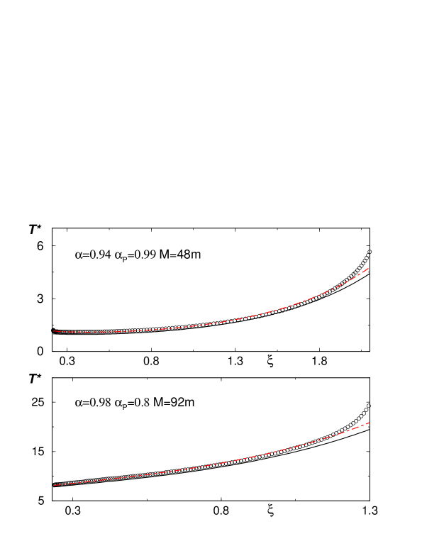
Figure 3: (Color online) Dimensionless temperature profile $T^{*}$ for the same two steady states as in Fig. 2. The solid line is the theoretical prediction given by Eq. (18) with the values of $A$ and $B$ determined in Sec. IV. The empty circles are MD results and the dashed line (red online) is the best fit to Eq. (18) by varying $A$ and $B$.

Similar degree of agreement has been found for all the studied combinations of parameters in the intervals $20\leq M/m\leq 120$, $0.9\leq\alpha<1$, and $0.6\leq\alpha_{P}\leq 1$. In particular, the inelasticity of the collisions between the movable piston and the grains, measured by the coefficient $\alpha_{P}$, seems to affect very weakly the accuracy of the theory.

It is interesting to plot also the hydrodynamic profiles in the original scale $z$ or, equivalently as a function of $z^{*}=zg_{0}/v_{W}^{2}$. In Fig. 4, the temperature profiles in the $z^{*}$-scale are shown for the same two steady states as in the previous figures. Also included are the profiles obtained with the best fitting parameters $A$ and $B$. It is observed that the agreement between theory and simulation is now worse than in the previous figures, where the spatial scale $\xi$ was employed. This is not at all surprising, since in the transformation of the theoretical prediction from the scale $\xi$ to the scale $z$, Eq. (10), the density profile is involved, and the ideal gas equation of state has been used. Consequently, the density effects discussed above manifest themselves in the transformation. Moreover, the scale $z$ is defined from $\xi$ in a cumulative way, as an integral over the density profile, so that the discrepancies increase as $z$ decreases. This effect is also clearly identified in Fig. 5, where the profiles for the reduced density $n^{*}$ are given. It is also seen that the simulation results extend to larger values of $z$ than the theoretical predictions for the profiles. It is worth to emphasize that the maximum value of the density, $n_{\max}$, remains quite low in both systems. For the system with $\alpha=0.94$, it is $n_{\max}\simeq 0.045\sigma^{-2}\simeq 0.039n_{c}$, while for the one with $\alpha=0.98$, $n_{\max}\simeq 0.04\sigma^{-2}\simeq 0.035n_{c}$.

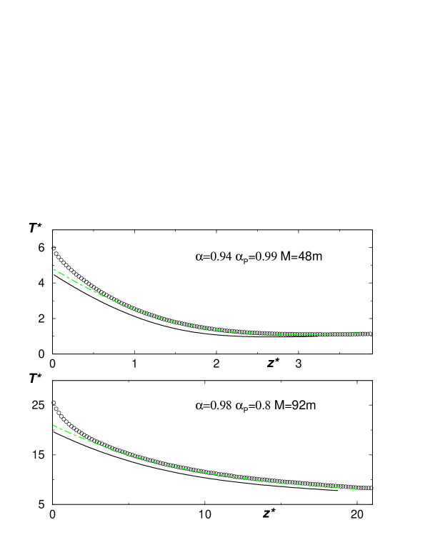
Figure 4: (Color online) Temperature profiles for the same systems as in Fig. 2, but now as a function of the reduced original coordinate $z^{*}$ defined in the text. The solid line is again the theoretical prediction with no adjustable parameters, and the symbols MD simulation results. The dotted-dashed lines (green online) have been obtained by fitting the two parameters $A$ and $B$ appearing in the expression of the temperature field using, moreover, the equation of state (82), as discussed in the main text.

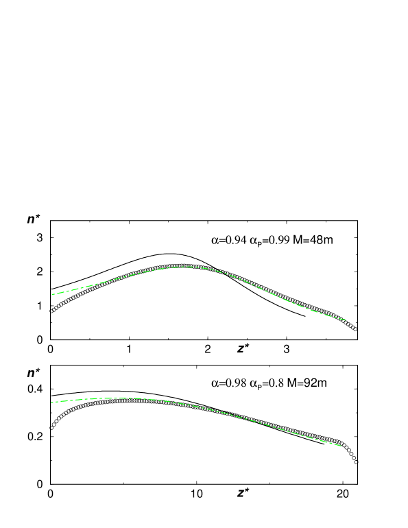
Figure 5: (Color online) Density profiles for the same systems as in Fig. 2 as a function of the reduced coordinate $z^{*}$ defined in the text. The solid line is the theoretical prediction with no adjustable parameters and the symbols MD simulation results. The dotted-dashed lines (green online) have been obtained by fitting the two parameters $A$ and $B$ appearing in the expression of the temperature field using, moreover, the equation of state (82), as discussed in the main text.

The previous analysis of the profiles in the $\xi$ variable suggests that the analytical expression of the reduced temperature in that variable is rather robust, in the sense of being very little affected by the finite density effects that, on the other hand, produce identifiable modifications on the pressure and density profiles. To check this idea, which can be useful to describe real experiments, the simulation profiles in Figs. 4 and 5 have been also fitted as follows. The pressure is given by Eq. (15), and for the temperature, $T(\xi)$, Eq. (18) is used, with $A$ and $B$ being adjustable parameters. Nevertheless, the equation of state is not that of an ideal gas, but Eq. (82). This equation of state is used both to compute the pressure from the simulation data, as discussed above, and also to transform from the $\xi$ coordinate to the $z$ one by means of Eq. (10). The profiles obtained in this way are also included in Figs. 4 and 5, and reproduce fairly well the hydrodynamic profiles in the bulk on the system.

V.2 Global properties and boundary conditions

The theoretical result for the average position of the piston $L$ is given by Eq. (80), with the density profile given by Eq. (20) and the values of the constants $A$ and $B$ following from Eqs. (75) and (77). In Fig. 6, the above prediction is compared with MD simulation results. The value of the dimensionless height $L^{*}=Lg_{0}/v_{W}^{2}$ as a function of $M/m$ is plotted for two systems, one with $\alpha=0.94$, $\alpha_{P}=0.99$, and the other one with $\alpha=0.99$, $\alpha_{P}=0.8$. The error bars in the simulations data have been obtained from the mean square fluctuations of the position of the piston around its average value, once in the steady state. Although there is a systematic underestimation of $L$, the agreement between theory and simulation is good over a quite wide range of values of the mass ratio. Prompted by the previous discussion of the hydrodynamic profiles, it is tempting to investigate whether some of the observed discrepancy is due to finite density corrections. Then, instead of using Eq. (20) for the density profile, the equation of state (82) was employed. In the latter, the pressure was given by Eq. (15) and the temperature by Eq. (18), with $A$ and $B$ still determined from Eqs. (75) and (77). The problem is that now the resulting expression for $L^{*}$ depends on the velocity of the bottom vibrating wall, $v_{W}$, and the simulation data in Fig. (6) have been obtained with different values of this velocity. For this reason, two different results are reported in the figure, corresponding to the two extreme values of $v_{W}$ used in the simulations. Although the dependence of the results on $v_{W}$ is small, it is clearly appreciable on the scale of the figure. As expected, the curve corresponding to the largest value of $v_{W}$ is the closest to the ideal gas prediction, since the larger $v_{W}$ the more dilute the system. Although some discrepancy between theory and simulation still persists, increasing as the value of $\alpha$ decreases, it seems fair to conclude the presence of finite density effects in the simulation results.

Figure 6: Average position of the piston $L^{*}$, measured in the dimensionless units defined in the text, as a function of the the mass ratio $M/m$, for two different pairs of the restitution coefficients $\alpha$, $\alpha_{P}$, as indicated in the figures. The symbols are MD simulation results and the solid lines the theoretical prediction derived in Sec. IV. The dashed lines and the dot-dashed lines have been obtained by using the equation of state (82), and correspond to the largest and smallest values of the velocity of the bottom wall $v_{W}$ used in the simulation, respectively.

Another relevant property characterizing globally the system is the power dissipated per unit of section $W$, as a consequence of the inelasticity of collisions. As discussed at the end of Sec. IV, this quantity is related with the heat flux at the boundaries by

$$D=Q_{L}-Q_{0}.$$ (83)

The fluxes $Q_{L}$ and $Q_{0}$ have been computed in Sec. IV by using approximate kinetic theory arguments and the expressions derived for them are given by Eqs. (66) and (68), respectively. These expressions are closed by means of Eqs. (69) and (70) and making, as above, the additional approximation $T_{P}/T_{L}\simeq 1$ in the expressions of $\phi$, Eq. (67).

In the MD simulations, $D$ is directly obtained from the loss of kinetic energy in each collision. In Fig. 7,

$$D^{*}\equiv\frac{\sigma D}{mg_{0}v_{W}}$$ (84)

is plotted as a function of $M/m$ for the same pairs of values $\alpha,\alpha_{P}$ as in Fig. 6. The agreement between theory and MD simulation is quite good. This provides strong additional support for the analysis of the boundaries carried out in Secs. III and IV and, consequently, for the boundary conditions employed in the hydrodynamic equations.

Figure 7: Dimensionless dissipated power $D^{*}$ per unit of transversal length in the steady state, as a function of the ratio between the mass of the piston, $M$, and the mass of the grains, $m$. The symbols are MD simulation results, while the lines have been obtained from the expressions of the fluxes at the boundaries derived in this paper. The circles and solid line correspond to systems with $\alpha=0.98$ and $\alpha_{P}=0.8$, and the squares and the dashed line to $\alpha=0.94$ and $\alpha_{P}=0.99$.

VI Conclusions

In this paper, the steady state of a fluidized granular gas of smooth inelastic hard spheres in presence of gravity, and with a movable lid on the top, has been investigated. It has been shown that, for weak inelasticity of the grain-grain collisions, the inelastic Navier-Stokes equations provide an accurate description of the density, temperature, and pressure profiles. For stronger inelasticity of the grains, a hydrodynamic description beyond the Navier-Stokes approximation is needed due to the coupling between gradients and inelasticity.

The issue of the required boundary conditions to solve the hydrodynamic equations has also been addressed. Here, the system was fluidized by means of a vibrating elastic wall at the bottom. For simplicity, it was assumed to move in a sawtooth way and with high frequency and small amplitude. The collisions of the particles with the piston on the top were modeled as smooth and inelastic. The above mechanical characterization of the walls was translated into exact boundary conditions for the joint distribution functions of each of the walls and the gas next to it. These kinetic boundary conditions are general, with restriction neither in the gas density nor in the inelasticity. They must be taken into account when finding approximate hydrodynamic boundary conditions. Otherwise, relevant exact properties, as the hydrodynamic meaning of the pressure of the gas at the boundaries, can be violated. Here, an approximation consistent with the kinetic boundary condition was developed and shown to lead to quite accurate results. It must be emphasized that the aim here has not been to analyze in detail the boundary layers next to the walls, but rather to identify the effective boundary conditions that must be satisfied by the hydrodynamic fields extrapolated to the boundaries from the bulk of the system.

Very recently, the so-called Knudsen temperature jump at a thermal wall has been incorporated at the Navier-Stokes equations of a weakly inelastic dilute gas of hard disks KMyS08 . As mentioned in the Introduction, thermal walls have not been proven to correspond to any well defined limit of vibrating walls. For the specific case of the inelastic piston on top of the system considered here, any analogy with a thermal wall seems very hard to justify. Moreover, the approximation followed in KMyS08 involves the determination of a constant prefactor by means of MD simulations, while here all the constants are determined by the theory.

The accuracy of the theoretical predictions has been checked by comparison with MD simulations. For some of the properties measured, e.g. the pressure profile, finite density effects have been identified and a practical way of accounting for them has been proposed. Of course, these effects could have been avoided by using the direct simulation Monte Carlo (DSMC) method Bi94 ; BRyC96 , instead of molecular dynamics. Nevertheless, the latter seems more appropriate in the present context, in which the interest focuses on the hydrodynamic description of a given state and not on a property of the Boltzmann equation. MD simulations provide results closer to real experiments since they are not based on the validity of any kinetic equation.

The interest has been on the description of the granular gas and its interaction with the piston. Of course, the study of the properties of the piston itself is also of great interest. For instance, its position fluctuations give the volume fluctuations of the gas. Some partial results have already been reported elsewhere ByR08 , but many points still deserve additional attention.

VII Acknowledgements

This research was supported by the Ministerio de Educación y Ciencia (Spain) through Grant No. FIS2008-01339 (partially financed by FEDER funds).

Appendix A Transport coefficients for a dilute granular gas

Here, the expressions of the dimensionless functions introduced in Sec. II are given for the sake of completeness. They read BDKyS98 ; ByC01

$$\kappa^{\ast}(\alpha)=[\nu^{\ast}_{2}(\alpha)-\frac{2d}{d-1}\zeta^{\ast}(\alpha)]^{-1}[1+c^{\ast}(\alpha)],$$ (85)

$$\mu^{\ast}(\alpha)=2\zeta^{\ast}(\alpha)\left[\kappa^{\ast}(\alpha)+\frac{(d-1)c^{\ast}(\alpha)}{2d\zeta^{\ast}(\alpha)}\right]\left[\frac{2(d-1)}{d}\nu^{\ast}_{2}(\alpha)-3\zeta^{\ast}(\alpha)\right]^{-1}\,,$$ (86)

$$\zeta^{\ast}(\alpha)=\frac{2+d}{4d}(1-\alpha^{2})\left[1+\frac{3}{32}c^{*}(\alpha)\right]\,,$$ (87)

where

$$\nu_{2}^{\ast}(\alpha)\equiv\frac{1+\alpha}{d-1}\left[\frac{d-1}{2}+\frac{3(d+8)(1-\alpha)}{16}+\frac{4+5d-3(4-d)\alpha}{1024}c^{\ast}(\alpha)\right],$$ (88)

$$c^{\ast}(\alpha)\equiv\frac{32(1-\alpha)(1-2\alpha^{2})}{9+24d+(8d-41)\alpha+30\alpha^{2}(1-\alpha)}\,.$$ (89)

These results have been obtained from the inelastic Boltzmann equation for hard spheres and disks by means of a generalized Chapman-Enskog algorithm, in the so-called first Sonine approximation BDKyS98 ; ByC01 .

Appendix B Calculation of the force exerted by the gas on the piston in the steady state

The force exerted by the granular gas on the piston equals the rate of momentum transferred from the gas to the piston in the collisions. When a particle collides with the piston, the amount of momentum given by the former to the latter is given by Eq. (26). Then, the average force on the piston $F_{z}$ is

$$F_{z} = \int d{\bm{x}}\int_{0}^{\infty}dZ\int_{-\infty}^{\infty}dV_{z}\,\Theta(g_{z})g_{z}\Delta P_{z}\Phi_{0,st}({\bm{x}},Z,V_{z})\delta(Z-z)$$ (90)

$$= \frac{mM}{m+M}\,(1+\alpha_{P})\int d{\bm{x}}\int_{0}^{\infty}dZ\int_{-\infty}^{\infty}dV_{z}g_{z}^{2}\Phi_{+,st}({\bm{x}},Z,V_{z})\delta(Z-z).$$

This expression can be rewritten in a more familiar form. First, decompose it as

$$F_{z} = m\int d{\bm{x}}\int_{0}^{\infty}dZ\int_{-\infty}^{\infty}dV_{z}\,v_{z}g_{z}\Phi_{+,st}({\bm{x}},Z,V_{z})\delta(Z-z)$$

$$-m\int d{\bm{x}}\int_{0}^{\infty}dZ\int_{-\infty}^{\infty}dV_{z}\,\left[v_{z}-\frac{M}{m+M}(1+\alpha_{P})g_{z}\right]g_{z}\Phi_{+,st}({\bm{x}},Z,V_{z})\delta(Z-z).$$

Next, taking into account Eq. (23), the second term on the right hand side of this equality is seen to be equivalent to

$$-m\int d{\bm{x}}\int_{0}^{\infty}dZ\int_{-\infty}^{\infty}dV_{z}\,v^{\prime}_{z}g_{z}\Phi_{+,st}({\bm{x}},Z,V_{z})\delta(Z-z)$$

$$=-m\int d{\bm{x}}^{*}\int_{0}^{\infty}dZ\int_{-\infty}^{\infty}dV_{z}^{*}\,v_{z}g_{z}^{*}\Phi_{+,st}({\bm{r}},{\bm{v}}^{*},Z,V_{z}^{*})\delta(Z-z)$$

$$=m\int d{\bm{x}}\int_{0}^{\infty}dZ\int_{-\infty}^{\infty}dV_{z}\,v_{z}g_{z}\Phi_{-,st}({\bm{x}},Z,V_{z})\delta(Z-z).$$ (92)

In the above transformations, ${\bm{x}}^{*}\equiv\{{\bm{r}},{\bm{v}}^{*}\}$ and the exact boundary condition in Eq. (41) has been employed. Substitution of Eq. (B) into Eq. (B) and use of the parity of $\Phi_{0,st}$ with respect to $V_{z}$ as well as its independence from ${\bm{r}}_{\perp}$ gives

$$F_{z} = m\int d{\bm{x}}\int_{0}^{\infty}dZ\int_{-\infty}^{\infty}dV_{z}\,v_{z}g_{z}\Phi_{0,st}({\bm{x}},Z,V_{z})\delta(Z-z)$$ (93)

$$= Wn_{L}T_{L,z},$$

where $n_{L}$ is the density of the granular gas next to the piston and $T_{L,z}$ a temperature parameter defined from the $z$-component of the velocity. Its expression is given in Eq. (48).

It is worth to stress that no assumption has been made over the properties of $\Phi_{0,st}$ other than the associated with the general symmetry properties of the steady macroscopic state under consideration and the boundary condition (41).

Appendix C The boundary condition at the vibrating wall

Accordingly with the description of the vibrating wall located at the bottom of the system given at the beginning of Sec. III, when a particle with velocity ${\bm{v}}$, being $v_{z}<0$, collides with this wall, its velocity is instantaneously changed into ${\bm{v}}^{\prime}$ defined by

$$v^{\prime}_{z}=2v_{W}-v_{z},\quad{\bm{v}}_{\perp}^{\prime}={\bm{v}}_{\perp},$$ (94)

Here, as already mentioned, $v_{W}$ is the (upwards) velocity of the wall and ${\bm{v}}_{\perp}$ is the vector component of ${\bm{v}}$ perpendicular to the $z$-axis. The kinetic energy gained by the particle in such a collision is

$$\Delta\epsilon=2m(v_{W}^{2}-v_{W}v_{z}).$$ (95)

For physical initial conditions in which there are no particles below the vibrating wall, the one-particle distributions function of the gas at arbitrary later times verifies

$$f({\bm{x}},t)=\Theta(z)f_{0}({\bm{x}},t),$$ (96)

where $f_{0}({\bm{x}},t)$ and its derivatives can be taken regular at $z=0$. Next, the above distribution function is decomposed at the wall as

$$f_{0}({\bm{x}},t)\delta(z)=f_{0}^{(+)}({\bm{x}},t)\delta(z)+f_{0}^{(-)}({\bm{x}},t)\delta(z),$$ (97)

with

$$f_{0}^{(\pm)}({\bm{x}},t)=\Theta(\pm v_{z})f_{0}({\bm{x}},t).$$ (98)

Conservation of the flux of particles at this wall is expressed by

$$f_{0}^{(-)}({\bm{x}},t)|v_{z}|\delta(z)d{\bm{v}}=f_{0}^{(+)}({\bm{x}}^{\prime},t)|v^{\prime}_{z}|\delta(z)d{\bm{v}}^{\prime},$$ (99)

where ${\bm{x}}^{\prime}\equiv\{{\bm{r}},{\bm{v}}^{\prime}\}$. Using Eqs. (94), the above relation can be transformed into

$$f_{0}^{(+)}({\bm{x}},t)v_{z}\delta(z)=f_{0}^{(-)}({\bm{x}}^{\prime},t)|v_{z}^{\prime}|\delta(z).$$ (100)

The heat flux at the vibrating wall, $Q_{0}$, is given by the rate of energy input per unit of section of the wall, i.e.

$$Q_{0}({\bm{r}}_{\perp},t) = \int dz\int d{\bm{v}}\ |v_{z}|\Delta\epsilon f_{0}^{(-)}({\bm{x}},t)\delta(z)$$ (101)

$$= \int dz\int{\bm{v}}\,mv_{z}^{2}v_{W}f_{0}^{(-)}({\bm{x}},t)\delta(z)\delta(z)$$

$$+\int dz\int d{\bm{v}}\,m|v_{z}|v_{W}|2v_{W}-v_{z}|f_{0}^{(-)}({\bm{x}},t)\delta(z).$$

Consider the second term on the right hand side of the above expression. Use of Eq. (100) yields

$$\int dz\int d{\bm{v}}\,m|v_{z}|v_{W}|2v_{W}-v_{z}|f_{0}^{(-)}({\bm{x}},t)\delta(z)=\int dz\int d{\bm{v}}\,mv_{z}^{2}v_{W}f_{0}^{(+)}({\bm{x}},t)\delta(z),$$ (102)

and substitution of this into Eq. (101) gives

$$Q_{0}({\bm{r}}_{\perp},t)=\int dz\int d{\bm{v}}\,mv_{z}^{2}v_{W}f_{0}({\bm{x}},t)\delta(z)=v_{W}n_{0}({\bm{r}}_{\perp},t)T_{0,z}({\bm{r}}_{\perp},t),$$ (103)

where

$$n_{0}({\bm{r}}_{\perp},t)\equiv\int dz\int d{\bm{v}}\,f_{0}({\bm{x}},t)\delta(z)$$ (104)

and

$$n_{0}({\bm{r}}_{\perp},t)T_{0,z}({\bm{r}}_{\perp},t)\equiv\int dz\int d{\bm{v}}\,mv_{z}^{2}f_{0}({\bm{x}},t)\delta(z).$$ (105)

Equation (68) in the main text follows by particularizing Eq. (103) for the one-dimensional steady state considered in this paper and assuming isotropy of the pressure tensor of the gas next to the vibrating wall.

The issue of the energy injected in a granular gas by means of an elastic vibrating wall moving in a sawtooth way has been addressed previously in ref. BRyM00 . The arguments there are restricted to a particular state with the gas modeled by means of Gaussian distributions. Moreover, although the results reported in BRyM00 are consistent with Eq. (103), the simplicity of this latter form of expressing the result was not realized there.

References

- (1) P.K. Haff, J. Fluid Mech. 134, 401 (1983).
- (2) C.S. Campbell, Annu. Rev. Fluid Mech. 22, 57 (1990).
- (3) I. Goldhirsch, Annu. Rev. Fluid. Mech. 35, 267 (2003).
- (4) C.K.W. Lun, S.B. Savage, D.J. Jeffrey, and N. Chepurniy, J. Fluid. Mech. 140, 223 (1984).
- (5) J.T. Jenkins and M.W. Richman, Arch. Ration. Mech. Anal. 87, 355 (1985); Phys. Fluids 28, 3485, (1986).
- (6) N. Sela and I. Goldhirsch, J. Fluid Mech. 361, 41 (1998).
- (7) J.J. Brey, J.W. Dufty, C.S. Kim, and A. Santos, Phys. Rev. E 58, 4638 (1998).
- (8) V. Garzó and J.W. Dufty, Phys. Rev. E 59, 5895 (1999).
- (9) J.J. Brey and J.W. Dufty, Phys. Rev. E 72, 011303 (2005).
- (10) J.J. Brey, M.J. Ruiz-Montero, and D. Cubero, Phys. Rev. E 54, 3664 (1996).
- (11) J.J. Brey and D. Cubero, in Granular Gases, edited by T. Pöschel and S. Luding (Springer-Verlag, Berlin, 2001).
- (12) Although not very recent, an interesting review and references can be found in: H.J. Hermann, in Third Granada Lectures in Computational Physics, edited by P.L. Garrido and J. Marro, Lectures Notes in Physics Vol. 448 (Springer-Verlag, Berlin, 1995), p. 67.
- (13) J.W. Dufty, A. Baskaran, and J.J. Brey, Phys. Rev. E 77, 031310 (2008).
- (14) A. Baskaran, J.W. Dufty, and J.J. Brey, Phys. Rev. E 77, 031311 (2008).
- (15) S. McNamara and J-L. Barrat, Phys Rev. E 55, 7767 (1997).
- (16) S. McNamara and S. Luding, Phys. Rev. E 58, 813 (1998).
- (17) J. Dorfman and H. van Beijeren, in Statistical Mechanics, Part B, edited by B. Berne (Academic, New York, 1977).
- (18) E.L. Grossman, T. Zhou, and E. Ben-Naim, Phys. Rev. E 55, 4200 (1997).
- (19) J.J. Brey and D. Cubero, Phys. Rev. E 57, 2019 (1998).
- (20) J.J. Brey, M.J. Ruiz-Montero, F. Moreno, and R. García-Rojo, Phys. Rev. E 65, 061302 (2002).
- (21) J.J. Brey, M.J. Ruiz-Montero, and F. Moreno, Phys. Rev. E 63, 061305 (2001).
- (22) Handbook of Mathematical Functions, edited by M. Abramowitz and I.A. Stegun (Dover, New York, 1965).
- (23) J.J. Brey and M.J. Ruiz-Montero, Europhys. Lett. 66, 805 (2004).
- (24) E. Clément and J. Rajchenbach, Europhys. Lett. 16, 133 (1991).
- (25) D.L. Blair and A. Kudrolli, Phys. Rev. E 67, 041301 (2003).
- (26) R.D. Wildman and J.M. Huntley, Power Tech. 182, 182 (2008).
- (27) J.F. Lutsko, Phys. Rev. Lett. 77, 225 (1999).
- (28) J.J. Brey, M.J. Ruiz-Montero, and F. Moreno, Phys. Rev. E 62, 5339 (2000).
- (29) S.R. Dahl, C.M. Hrenya, V. Garzó, and J.W. Dufty, Phys. Rev. E 66, 041301 (2002).
- (30) R. D. Wildman and D.J. Parker, Phys. Rev. Lett. 88, 064301 (2002).
- (31) K. Feitosa and N. Menon, Phys. Rev. Lett. 88, 198301 (2002).
- (32) J.J. Brey and M.J. Ruiz-Montero, J. Stat. Mech. L09002 (2008).
- (33) E. Livne, B. Meerson, and P.V. Sasorov, Phys. Rev. E 66, 050301 (2002).
- (34) E. Khain, B. Meerson, and P.V. Sasorov, Phys. Rev. E 78, 041303 (2008).
- (35) G. Bird, Molecular Gas Dynamics and the Direct Simulation of Gas Flows (Clarendon Press, Oxford, 1994).