Fast Cycle Frequency Domain Feature Detection for Cognitive Radio Systems

Abstract

In cognitive radio systems, one of the main requirements is to detect the presence of the primary users’ transmission, especially in weak signal cases. Cyclostationary detection is always used to solve weak signal detection, however, the computational complexity prevents it from wide usage. In this paper, a fast cycle frequency domain feature detection algorithm has been proposed, in which only feature frequency with significant cyclic signature is considered for a certain modulation mode. Simulation results show that the proposed algorithm has remarkable performance gain than energy detection when supporting real-time detection with low computational complexity.

I Introduction

The remarkable growth of wireless services over the last decade demonstrates the vast and increasing demand for radio spectrum. However, the spectrum resource is limited and most has been licensed exclusively to users which can work within a limited frequency band. Recent study [1] shows that the actual licensed spectrum is largely unoccupied most of the time. Thus, cognitive radio (CR) has been proposed to solve this problem [2], [3]. By sensing and adapting to the environment, CR users are able to fill in spectrum holes and serve its users without causing harmful interference to the licensed user. Therefore, the CR system requires spectrum sensing technique that detects the unoccupied spectrum band as quickly and accurately as possible for its implementation.
Various spectrum sensing techniques have been presented including matched filter, energy detection and cyclostationary detection [4-7]. Matched filter requires perfect knowledge of the primary users’ signal features. Energy detection method is sensitive to noise and interference level. As an alternative, cyclostationary detection has a good performance in low SNR scenarios, but it costs a large amount of computational capacity, which makes it not suitable for real-time detection [8]. In this paper, a fast cycle frequency domain feature detection algorithm has been proposed, in which only feature frequency with significant cyclic signature is considered for a certain modulation mode. The detection performance and computational complexity for the proposed algorithm are analyzed and compared with those of energy detection.
The rest of this paper is organized as follows: The system model under consideration is discussed in Section II. Section III gives a brief overview of cyclostationary spectrum analysis. Section IV introduces the proposed algorithm. Simulation results and performance comparison with energy detection are given in Section IV. Finally, conclusions are drawn in Section V.

II SYSTEM MODEL

The spectrum sensing problem can be modeled as hypothesis testing. It is equivalent to distinguishing between the following two hypotheses:

$$\left\{\begin{array}[]{l}H_{0}:y(t)=n(t)\\ H_{1}:y(t)=x(t)+n(t)\\ \end{array}\right.$$ (1)

$y(t)$,$x(t)$and $n(t)$ denote the received signal, the primary user’s transmit signal, and the noise, respectively. $H_{1}$ and $H_{0}$ represent the hypothesis that the primary user is active or inactive. Due to the existence of noise, a certain threshold $\lambda_{{\rm{th}}}$ should be set to decide whether a primary user is active or not. Probability of detection ($P_{d}$) and false alarm ($P_{f}$) are defined to evaluate the detection performance:

$$\left\{\begin{array}[]{l}P_{d}=p({\rm{y}}_{i}>\lambda_{{\rm{th}}}\left|{H_{1}}\right.)\\ P_{f}=p(y_{i}>\lambda_{{\rm{th}}}\left|{H_{0}}\right.)\\ \end{array}\right.$$ (2)

The goal of detection is to maximize the $P_{d}$ while maintain a given $P_{f}$.

III CYCLOSTATIONARY SPECTRUM ANAYSIS

The cyclic autocorrelation of a complex-valued time series $x(t)$ is defined by [7]:

$$R_{x}^{\alpha}\left(\tau\right)\buildrel\Delta\over{=}\mathop{\lim}\limits_{T\to\infty}\frac{1}{T}\int\limits_{-\frac{T}{2}}^{\frac{T}{2}}{x\left({t+\frac{\tau}{2}}\right)}x^{*}\left({t-\frac{\tau}{2}}\right)e^{-i2\pi\alpha t}dt$$ (3)

where $\alpha$ is referred to as the cycle frequency.
The Spectral Correlation Density (SCD) of $x(t)$, which is also known as the cyclic spectrum, can be obtained by Fourier transforming the cyclic autocorrelation

$$S_{x}^{\alpha}\left(f\right)=F\left\{{R_{x}^{\alpha}\left(\tau\right)}\right\}=\int\limits_{-\infty}^{\infty}{R_{x}^{\alpha}\left(\tau\right)}e^{-i2\pi f\tau}d\tau$$ (4)

If $x(t)$ is Additive White Gaussian Noise (AWGN), then when $\alpha\neq 0$,$S_{x}^{\alpha}(f)=0$.
The frequency-smoothing method is adopted to estimate SCD, and the discrete formulation can be expressed as [9] [10]:

$$\begin{array}[]{l}\tilde{S}_{x}^{\alpha}\left[l\right]=\frac{1}{{\left({N-1}\right)T_{s}}}*\\ \frac{1}{L}\sum\limits_{v=\frac{{-\left({L-1}\right)}}{2}}^{v=\frac{{L-1}}{2}}{X\left({l+\frac{\alpha}{{2F_{s}}}+v}\right)X^{*}\left({l-\frac{\alpha}{{2F_{s}}}+v}\right)W\left(v\right)}\\ \end{array}$$ (5)

where

$$X\left[v\right]=\sum\limits_{k=0}^{N-1}{x\left[k\right]}e^{-i2\pi vk/N}$$ (6)

$N$ is the number of input signal samples, $x\left[k\right]=x\left({kT_{\rm{s}}}\right)$, $T_{\rm{s}}$ is the time-sampling increment, $F_{s}={\raise 3.01385pt\hbox{$1$}\!\mathord{\left/{\vphantom{1{NT_{s}}}}\right.\kern-1.2pt}\!\lower 3.01385pt\hbox{${NT_{s}}$}}$ is the frequency-sampling increment, $l=\left\lfloor{{\raise 3.01385pt\hbox{$f$}\!\mathord{\left/{\vphantom{f{F_{s}}}}\right.\kern-1.2pt}\!\lower 3.01385pt\hbox{${F_{s}}$}}}\right\rfloor$ is the discrete value of the frequency, and $W\left(v\right)$ is the frequency-smoothing function centered at $v=0$ of width $L$ .

IV Cycle Frequency Domain Feature Detection Algorithm

The Spectral Correlation Density (SCD) of a signal is a cross-correlation function between frequency components separated by $f+\frac{\alpha}{2}$and $f-\frac{\alpha}{2}$, we mapped it from $f\sim\alpha$ square to $\alpha$ axis through the following expression

$$I_{x}\left(\alpha\right)=\mathop{\max}\limits_{f}|S_{x}^{\alpha}\left(f\right)|$$ (7)

And $I_{x}\left(\alpha\right)$ can be regarded as the SCD of a signal at the cyclic frequency domain. Different signal modulations will exhibit different cyclic features in the cyclic frequency domain, as shown in Figure 1 and 2. AM and BPSK modulated signals both have significant features at $\alpha_{0}=2f_{c}$.

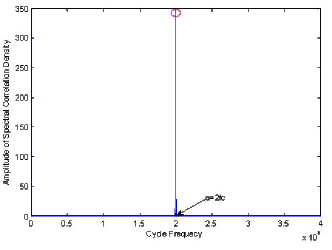
Figure 1: Cycle Frequency Domain for AM signal

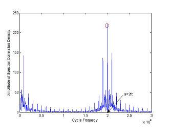
Figure 2: Cycle Frequency Domain for BPSK signal

The cyclic features of a signal are decided by the modulation types it employed. From the experiment results we found that there exists a significant feature at $\alpha_{0}=2f_{c}$ for both analog and digital amplitude modulated signals, where the carrier frequency is $f_{c}$. In the following section of this paper, only SCD of the most significant features ($\alpha_{0}$) of a modulated signal will be considered when performing detection.
We assume that the modulation type and the carrier frequency $f_{c}$ of the signal are known, namely the cycle frequency $\alpha_{0}=2f_{c}$ is known to us. After SCD estimation at cycle frequency $\alpha_{0}$ , the system detection model (1) changes into the following form:

$$\left\{\begin{array}[]{l}H_{0}:\tilde{S}_{y}^{\alpha_{0}}(l)=\tilde{S}_{n}^{\alpha_{0}}(l)\\ H_{1}:\tilde{S}_{y}^{\alpha_{0}}(l)=\tilde{S}_{x}^{\alpha_{0}}(l)+\tilde{S}_{n}^{\alpha_{0}}(l)\\ \end{array}\right.$$ (8)

The cyclostationary spectrum sensing metric of the received signal is obtained by

$$M=\mathop{\max}\limits_{l}\left|{\tilde{S}_{y}^{\alpha_{0}}\left(l\right)}\right|$$ (9)

A. When the primary user is inactive ( $H_{0}$ hypothesis), the sensing metric becomes

$$M_{0}=\mathop{\max}\limits_{l}\left|{\tilde{S}_{y}^{\alpha_{0}}\left(l\right)}\right|=\mathop{\max}\limits_{l}|\tilde{S}_{n}^{\alpha_{0}}\left(l\right)|$$ (10)

Theoretically, $n(t)$ is AWGN, so when $\alpha_{0}\neq 0$, $\tilde{S}_{n}^{\alpha_{0}}(l)=0$, $M_{0}=0$. However, for Limited length SCD, when $\alpha_{0}\neq 0$, $\tilde{S}_{n}^{\alpha_{0}}(l)\neq 0$, $M_{0}\neq 0$ [11].
B. When the primary user is active ($H_{1}$ hypothesis), the sensing metric becomes

$$\begin{array}[]{l}M_{1}=\mathop{\max}\limits_{l}|\tilde{S}_{y}^{\alpha_{0}}(l)|\\ {\rm{}}=\mathop{\max}\limits_{l}|\tilde{S}_{x}^{\alpha_{0}}(l)+\tilde{S}_{n}^{\alpha_{0}}(l)|\\ {\rm{}}=\mathop{\max}\limits_{l}\left({|\tilde{S}_{x}^{\alpha_{0}}(l)|+|\tilde{S}_{n}^{\alpha_{0}}(l)|}\right)\\ {\rm{}}\mathop{\approx\max}\limits_{l}|\tilde{S}_{x}^{\alpha_{0}}(l)|+\mathop{\max}\limits_{l}|\tilde{S}_{n}^{\alpha_{0}}(l)|\\ {\rm{}}=\mathop{\max}\limits_{l}|\tilde{S}_{x}^{\alpha_{0}}(l)|+M_{0}\\ \end{array}$$ (11)

The decision on the presence of a primary user is simplified to distinguish $M_{0}$ from $M_{1}$. when the sensing metric of the receiving signal is M, namely decide the channel belongs to $H_{0}$ or $H_{1}$. A decision threshold $\lambda_{th}$ is set to classify the metric M:

$$\left\{\begin{array}[]{l}M_{0}(H_{0}):\begin{array}[]{*{20}c}{}\hfil\\ \end{array}if\begin{array}[]{*{20}c}{M<\lambda_{th}}\\ \end{array}\\ M_{1}(H_{1}):\begin{array}[]{*{20}c}{}\hfil\\ \end{array}if\begin{array}[]{*{20}c}{M>\lambda_{th}}\\ \end{array}\\ \end{array}\right.$$ (12)

Probability of detection $P_{d}$ and probability of false alarm $P_{f}$ then be formulated as

$$\left\{{\begin{array}[]{*{20}c}{P_{d}=\Pr(M>\lambda_{{\rm{th}}}|H_{1})}\\ {P_{f}=\Pr(M>\lambda_{th}|H_{0})}\\ \end{array}}\right.$$ (13)

The threshold $\lambda_{th}$ can be selected for finding an optimum balance between $P_{d}$ and $P_{f}$ .

V SIMULATION RESULTS

In this section, Monte Carlo simulation results are presented to show the better detection performance for the proposed algorithm when comparing with energy detection. Simulation parameters are listed in TABLE 1.

TABLE I: Simulation parameters list

Parameter	Value
Modulation type	AM
Carrier frequency	1 MHz
Bandwidth	10 KHz
Sampling frequency	3 MHz
Sampling time	1.365ms
Channel	AWGN
Window type	hamming
Frequency smoothing length(L)	1300
Sampled data length(N)	4096

Figure 3 shows the curves of receiver operating characteristics (ROC) of the proposed method and energy detection, it’s obvious that the proposed method outperforms the energy detection algorithm.
Energy detection performs badly when SNR bellows -17db, while proposed method still has a good performance under even -22db. For example, when SNR equals to -22db and the probability of false alarm ($P_{f}$) is 0.1, the probability of detection ($P_{d}$) of the proposed method and energy detection equal to 0.99 and 0.18, respectively; when $P_{f}=0.01$ , the two $P_{d}$ change to be 0.93 and 0.25, respectively. A cognitive radio operation in licensed TV bands (IEEE 802.22 working group) defines ”required SNR sensitivity” for primary user signals to be: -22dB for DTV signals and -10 dB for wireless microphones [12]. Therefore, the proposed method meets the requirements well.

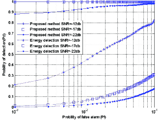
Figure 3: Performance comparison between the proposed method and energy detection

If we choose FFT to deal with the formulation (5) and use the following expression to calculate the energy of a signal ($E_{x}$), the complexity of the two methods are shown in table 2.

$$E_{x}=\sum\limits_{i=1}^{N}{x\left(i\right)}x^{*}\left(i\right)$$ (14)

where $x(i)$ is the sample of a signal, N is the sample number.

TABLE II: Complexity comparison between the proposed method and energy detection

	The proposed method	Energy detection
Real multiply	$2N\log_{2}N+5L$	$4N$
Real add	$3N\log_{2}N+3L$	$3N$

From Table 2, we can see that the complexity of the proposed method is approximately $\log_{2}N$ times of energy detection. The main computation consumption is from FFT calculation in the method, for a modern FFT chip this is not a big matter as if N is not too big. So the more extra computation complexity of the proposed method than energy detection is worthy, when considering the performance it achieves. To achieve better detection performance, energy detection demands much longer sampling time [13], which is not necessary for the proposed method. Therefore, the proposed Fast Cycle Frequency Domain Feature Detection algorithm support real-time detection as well.

VI Conclusion

In this paper, a fast cycle frequency domain feature detection algorithm is proposed, in which only feature frequency with significant cyclic signature is calculated. Compared to the traditional implementation of cyclostationary detection, computation complexity for the proposed algorithm is greatly reduced under the finite prior knowledge of modulation type and carrier frequency. Simulation results show that the detection performance of the proposed method outperforms that of energy detection. Therefore, the proposed method is more suitable for real time spectrum sensing in cognitive radio system.

References

- [1] Federal Communications Commission, ”Spectrum policy task force report”, ET Docket No.02-135, Nov. 2002.
- [2] J. Mitola and G. Q. Maguire, ”Cognitive radio: making software radios more personal,” IEEE Pers. Commun., vol. 6, pp. 13-18, Aug. 1999.
- [3] S. Haykin, ”Cognitive radio: brain-empowered wireless communications,” IEEE J. Select. Areas Commun., vol. 23, pp. 201-220, Feb. 2005.
- [4] Danijela Cabric, Shridhar Mubaraq Mishra, Robert W. Brodersen, ”Implementation issues in spectrum sensing for cognitive radios”, Asilomar Conference on Signal, Systems and Computers, pp.772-774, (2004).
- [5] Ian F. Akyildiz, Won-Yeo Lee, Mehmet C. Vuran, Shantidev Mohanty, ”Next generation/dynamic spectrum access/cognitive radio wireless networks: a survey”, Computer Networks, Vol.50, pp. 2127 - 2159, (2006).
- [6] W. Gardner, ”The spectral correlation theory of cyclostationary time-series”, Signal Processing, Vol.11(1), pp.13-36, (1986).
- [7] W. A. Gardner, Introduction to Random Processes with Applications to Signals and Systems. New York: Macmillan, 1986.
- [8] Gan Xiaoying, Xu Hao, Xu Youyun, Qian Liang, Liu Jing, ”Noise analysis for limited length cyclostationary detection in cognitive radio systems”, Journal of PLA University of Science and Technology,2008. vol. 9, No.6, pp:633-636.
- [9] W.A. Gardner, ”Measurement of Spectral Correlation”, IEEE Trans. on Acoustics, Speech, and Signal Processing, VOL. ASSP-34, NO. 5, Oct. 1986.
- [10] W.A. Gardner, ”Digital Implementations of Spectral Correlation Analyzers”, IEEE Trans. on Signal Processing, VOL 41, NO 2, Feb. 1993.
- [11] Gan Xiaoying, Xu Hao, Xu Youyun, Qian Liang, Liu Jing, Noise analysis for limited length cyclostationary detection in cognitive radio systems , Journal of PLA University of Science and Technology,2008, vol. 9, No.6, pp:633-636.
- [12] G. Chuinard, D. Cabric, and M. Ghosh, ”Sensing thresholds,” Tech. Rep. IEEE 802.22-06/005/r3, May 2006
- [13] Danijela Cabric, Artem Tkachenko and Robert W. Brodersen, ”Experimental study of spectrum sensing based on energy detection and network cooperation”, ACM 1st Int’l. Workshop on Technology and Policy for Accessing Spectrum (TAPAS), August 2006.