A turbulent model for the surface brightness of extragalactic jets

Este documento describe ..

Abstract

This paper summarizes the known physics of turbulent jets observed in laboratory experiments. The formula, which gives the power released in turbulence describes the concentration of turbulence/relativistic particles in each point of the astrophysical jets. The same expression is also used to analyze the power released in turbulence in the case of pipe and non Newtonian fluids. Through an integral operation it is possible to deduce the intensity of synchrotron radiation for a profile perpendicular or not to a straight jet , a 2D map for a perpendicular , randomly oriented straight jet as well as a 2D map of complex trajectories such as NCC4061 and 3C31. Presented here is a simulation of the spectral index in brightness of 3C273 as well as a 2D map of the degree of linear polarization. The Sobel operator is applied to the theoretical 2D maps of straight perpendicular jets.

galaxies :jets radio continuum : galaxies

0.1 Introduction

The physical mechanism that leads to the formation of the image in extra-galactic radio-sources can be the same which explains the physics of such objects ; this is called the unique model. The unique model can be split in two

1. The extremely relativistic, mono-energetic $e\pm$–pairs of high bulk Lorentz factor, see Kundt (1979); Kundt & Gopal Krishna (2004); Kundt (2006).

2. On modeling the jets as intrinsically symmetrical, relativistic, decelerating flows it is possible to simulate the radio-map of 3C31, 0326+39,1553+24 , NGC 315 and 3C296, see Laing & Bridle (2002a); Canvin & Laing (2004); Laing et al. (2005, 2006); Worrall et al. (2007).

The transport processes are an open rather than a well established field of research. Following is a brief review of some approaches.

1. The Kelvin-Helmholtz instabilities trigger a fluid turbulent cascade. The electrons are accelerated from the low wavelength of the turbulent spectrum , see Ferrari et al. (1979); Eilek et al. (2003).

2. The laws of blob containment , see Zaninetti (1989) , or the 3D random walk , see Zaninetti (1999) , produce simulated maps of radiation intensity from extra-galactic radio-sources.

3. Plasma instabilities (e.g., Buneman, Weibel, and other two-stream instabilities) created in collision-less shocks may be responsible for particle (electron, positron) acceleration, see Nishikawa et al. (2006).

The canonical approach to the turbulence is through the Navier-Stokes equations

$$\frac{D{\bf U}}{Dt}=\frac{1}{\rho}\nabla p+\nu\nabla^{2}{\bf U}\quad,$$ (1)

where ${\bf U}$ represents the velocity vector , $\frac{D{\bf U}}{Dt}$ is the fluid particle acceleration , $\nu$ is the kinematic viscosity, $\rho$ the density and $p$ the pressure. By applying the Reynolds decomposition to the previous equations

$${\bf U(x,t)}=\langle{\bf U(x,t)}\rangle+{\bf u(x,t)}\quad,$$ (2)

where ${\bf u(x,t)}$ represents the fluctuation, we obtain the equation of the mean momentum or Reynolds equations

$$\frac{{\overline{D}}{U_{j}}}{\partial t}=-\nu\nabla^{2}(U_{j})-\frac{\partial\langle u_{i}u_{j}\rangle}{\partial x_{i}}-\frac{1}{\rho}\frac{\partial\langle p\rangle}{\partial x_{i}}\quad,$$ (3)

where $\frac{{\overline{D}}}{\partial t}$ represents the mean substantial derivative. The difference between the Reynolds and the Navier-Stokes equations is represented by the Reynolds stresses , $\frac{\partial\langle u_{i}u_{j}\rangle}{\partial x_{i}}$. The following reviews three different models which adopt the turbulence in astrophysical jets.

1. A complex approach to the turbulence is through the ensemble by Favre (1969) , see Bicknell (1984) , where the density $\rho$ is expressed as $\rho+\rho^{\prime}$ and the velocity $v_{i}$ as $v_{i}+v_{i}^{\prime}$ where ($i=1,2,3$). From this double decomposition it is possible to obtain four equations for mass , momentum , turbulent kinetic energy and heat. The behavior of the magnetic field is obtained by taking into consideration the ensemble average of the MHD equations for the magnetic field $B_{i}$ in the infinite conductivity limit. Once a law for the pressure of the atmosphere is considered, it is possible to obtain a law for the velocity , the electron distribution function , the magnetic field dependence and the density. The above equations allow us to deduce a law for the brightness along the jet $I_{\nu}^{\prime}$ once an adimensional opening angle , $a^{\prime}=\phi/\phi_{0}$ , is introduced. The brightness law is of the type $I_{\nu}^{\prime}\propto a^{-b}$ with $b\leavevmode\nobreak\ [0.35-0.78]$ . In this model the opening angle is variable , and the application was done to $3C31$ which shows a variable opening angle starting from $12.3^{\circ}$ , reaching a maximum of $16.6^{\circ}$ in the middle and re-collimating in the outer regions at $12.6^{\circ}$ , see Table 1 in Bridle et al. (1980). Another application of this model was the study of the physical state of the interstellar medium in the optical counterpart NGC 383.

2. A compressible k-e turbulence model was used by Falle (1994) to study the effect of turbulence on the propagation of fluid jets. In this model a connection between the opening angle of the jet $\theta$ and the Mach number , $M$ , is

   $$M=\frac{1}{\theta}\quad.$$ (4)

   Through a numerical simulation the z-component of velocity along a cut perpendicular to the z-axis has been evaluated.

3. The near infrared images of HH 110 jet (Herbig Haro) were interpreted as due to low velocity shocks produced by turbulent processes, see  Noriega-Crespo et al. (1996). The spatial intensity distribution of $H_{2}$ , $H_{\alpha}$ and $[S_{II}]_{617/31}$ perpendicular to the flow axis and along the cross section of knots in $HH110$ has a behavior that can be approximated by a Gaussian distribution , see Figure 4 in Noriega-Crespo et al. (1996). In one case , $H_{\alpha}$ in knot P of HH110, it is possible to see a bump near the maximum of the intensity in the transversal direction. This can be considered the first observational evidence of a physical effect which will , later on , be called ” valley on the top” . The results were explained by Noriega-Crespo et al. (1996) adopting a turbulent mixing layer that followed a Couette flow.

The previous approaches do not solve the following questions

• Can the physics of turbulent jets , which are observed in the laboratory, be applied to extra-galactic radio-sources ?

• Is it possible to build the image of a straight turbulent jet which is emitting synchrotron radiation from the law of dissipation of turbulence ?

• Could the observed cuts in non-thermal radiative flux, parametrized as a function of the distance , be compared with theoretical cuts ?

• Could the 2D maps in brightness that characterize the complex morphologies associated with radio-galaxies be simulated ?

• Is it possible to simulate the variation of the spectral index in brightness of the non-thermal emission ?

The previous cited papers on turbulence solve some of the problems connected with the application of turbulence to astrophysical jets but leave other problems open and Table 1 reports the status.

Table 1: Synoptic table of the solved and unsolved problems in three different turbulence papers and here

$$\begin{array}[]{lcccc}\hline\cr\hline\cr\vskip 3.0pt plus 1.0pt minus 1.0pt\cr Problem&Bicknell\leavevmode\nobreak\ 1984&Falle\leavevmode\nobreak\ 1994&Noriega-Crespo\leavevmode\nobreak\ et\leavevmode\nobreak\ al.\leavevmode\nobreak\ 1996&this\leavevmode\nobreak\ paper\\ \vskip 3.0pt plus 1.0pt minus 1.0pt\cr\hline\cr\vskip 3.0pt plus 1.0pt minus 1.0pt\cr brightness\leavevmode\nobreak\ along\leavevmode\nobreak\ the\leavevmode\nobreak\ jet&yes&not&not&yes\\ perpendicular\leavevmode\nobreak\ brightness&not&not&not&yes\\ image\leavevmode\nobreak\ as\leavevmode\nobreak\ integral\leavevmode\nobreak\ operation&not&not&not&yes\\ law\leavevmode\nobreak\ for\leavevmode\nobreak\ magnetic\leavevmode\nobreak\ field&yes&not&not&not\\ valley\leavevmode\nobreak\ on\leavevmode\nobreak\ the\leavevmode\nobreak\ top&not&not&yes&yes\\ \vskip 3.0pt plus 1.0pt minus 1.0pt\cr\vskip 3.0pt plus 1.0pt minus 1.0pt\cr\hline\cr\hline\cr\end{array}$$

This paper briefly introduces in Section 0.2 an approximate law for the conversion of energy of the bulk flow into the turbulent cascade and the radiative transfer equation. Section 0.3 computes the power released in the turbulent cascade for three type of fluids : turbulent fluid , pipe fluid and non-Newtonian fluid. Section 0.4 computes through an integral, the intensity profiles of the jet when it is directed in the direction perpendicular to the motion for the three types of fluids previously analyzed.

Section 0.5 deals with an algorithm used to build the synchrotron image in two simple cases : the straight jet is oriented in the direction perpendicular to the observer or has a random direction.

Section 0.6 presents the images of the radio-jets which present bending and wiggling , such as NGC4061 and 3C31. This Section also contains a simulation of the spectral index in brightness of turbulent astrophysical jets.

0.2 Preliminaries to the radio–images

Section 0.2.1 analyzes a possible mechanism for conversion of energy from the flux of kinetic energy down to the turbulence. The matrix equation that implements the radiative transfer equation is introduced in Section 0.2.2 .

0.2.1 The efficiency of energy conversion

The total power , $Q$ , released in a turbulent cascade of the Kolmogorov type is, see Pelletier & Zaninetti (1984)

$$Q\approx\gamma_{KH}\rho s_{T}^{2}\quad,$$ (5)

where $\gamma_{KH}=\gamma_{ad}\frac{s_{T}}{a}$ is the growth rate of K–H instabilities , $\rho$ is the matter density and $s_{T}$ is the sound velocity, see Section 9.1 in Zaninetti (2007).

The total maximum luminosity , $L_{t}$ , which can be obtained for the jet in a given region of radius $a_{j}$ and length $a_{j}$ is

$$L_{t}=\pi a_{j}^{2}a_{j}Q=\gamma_{ad}\rho s_{T}^{3}\pi a_{j}^{2}\quad.$$ (6)

The mechanical luminosity of the jet is

$$L_{m}=\frac{1}{2}\rho v^{3}\pi a_{j}^{2}\quad,$$ (7)

and therefore the efficiency of the conversion , $\chi_{T}$ , of the total available energy in turbulence is

$$\chi_{T}=\frac{L_{t}}{L_{m}}=\gamma_{ad}\frac{2}{\pi}\frac{1}{M^{3}}\approx\frac{1}{M^{3}}\quad,$$ (8)

where $M$ is the Mach number. From this equation it is clear that the fraction of the total available energy released firstly in the turbulence and after in non thermal particles is a small fraction of the bulk flow energy. The assumption made in Section 3 and Section 4 by Zaninetti (2007) in which the bulk flow motion was treated independently from non–thermal emission is now justified.

0.2.2 Radiative transfer equation

The transfer equation in the presence of emission only , see for example Rybicki & Lightman (1985), is

$$\frac{dI_{\nu}}{ds}=j_{\nu}\quad,$$ (9)

where $I_{\nu}$ is the specific intensity , $s$ is the line of sight , $j_{\nu}$ the emission coefficient, and the index $\nu$ denotes the interested frequency of emission. The solution to equation (9) is

$$I_{\nu}(s)=I_{\nu}(s_{0})+\int_{s_{0}}^{s}j_{\nu}(s\prime)ds\prime\quad,$$ (10)

where $I_{\nu}(s_{0})$ represents the intensity at $s=s_{0}$ , in this case zero. In the case of synchrotron emission, the maximum intensity of mono-energetic electrons in the presence of a magnetic field $B$ in gauss is

$$I_{\nu}(s)=1.710^{-23}B_{\bot}\int C(s)ds\leavevmode\nobreak\ \leavevmode\nobreak\ \leavevmode\nobreak\ \frac{erg}{cm^{2}\leavevmode\nobreak\ s\leavevmode\nobreak\ sr\leavevmode\nobreak\ Hz}\quad,$$ (11)

where $C(s)$ is the number of electrons in a unit volume along the line of sight and $B_{\bot}$ is the component of $B$ perpendicular to the velocity vector , see for example equation (5.550) in Ginsburg (1975). In the case of spatial dependence on $j_{\nu}$ it is assumed

$$j_{\nu}=C_{j}C(s)\quad,$$ (12)

where

$$C_{j}=1.710^{-23}B_{\bot}\leavevmode\nobreak\ \leavevmode\nobreak\ \leavevmode\nobreak\ \frac{erg}{\leavevmode\nobreak\ s\leavevmode\nobreak\ sr\leavevmode\nobreak\ Hz}\quad.$$ (13)

The intensity in the non-homogeneous case is

$$I_{\nu}(s)=C_{j}\int_{s_{0}}^{s}C(s\prime)ds\prime\quad.$$ (14)

The increase in brightness is proportional to the concentration integrated along the line of sight. In the Monte Carlo experiments here analyzed, the concentration is memorized on the three-dimensional grid ${\mathcal{C}}$ and the intensity is

$${\it I}(i,j)=\sum_{k}\delta\times{\mathcal{C}}(i,j,k)\quad,$$ (15)

where $\delta$ is the spatial interval between the values of concentration and the sum is performed over the interval of existence of index k.

0.3 Three types of fluids

The cases of shear layer produced by a turbulent jet, by a pipe and by a non-Newtonian fluid are now analyzed.

0.3.1 The turbulent jet

The theory of turbulent round jets can be found in different textbooks. The more important formulas are now reviewed as extracted from chapter V by Pope (2000) ; similar results can be found in Bird et al. (2002) and in Schlichting et al. (2004) . We start with the centerline velocity $U_{0}(z)$ , equation (5.6) in Pope (2000) , as measured in the laboratory experiments :

$$\frac{U_{0}(z)}{U_{1}}=\frac{B}{z/d}\quad,$$ (16)

here $z$ denotes the main direction , $d$ is the diameter of the nozzle, $B$ is a constant derived in the laboratory that takes the value 5.8, and $U_{1}$ is the initial jet velocity. The solution of the mean velocity $<U>$ , equation (5.100) in Pope (2000) , along the main direction is

$$<U>=U_{1}\frac{8a_{T}\nu_{T}}{z}\frac{1}{(1+a_{T}\eta^{2})^{2}}\quad,$$ (17)

where $\eta=\frac{r}{z}$ , $r$ is the radius of the jet at $z$, $a_{T}$ is a constant and $\nu_{T}$ is the turbulent viscosity. The viscosity , equation (5.104) in Pope (2000) , is

$$\nu_{T}=\frac{S}{8(\sqrt{2}-1)}\quad,$$ (18)

and $a_{T}$, equation (5.18) in Pope (2000), is

$$a_{T}=\frac{(\sqrt{2}-1)}{S^{2}}\quad,$$ (19)

where $S$ will be later defined. The production of turbulent kinetic energy in the boundary layer approximation , equation (5.145) in Pope (2000) , is

$$\mathcal{P}=\nu_{T}(\frac{\partial<U>}{\partial y})^{2}\quad,$$ (20)

where $y$ is a Cartesian coordinate that can be identified with $r$. The flow rate of mass $m(z)$ is , see equation (5.68) in Pope (2000) ,

$$\dot{m(z)}=2\pi\rho b_{1/2}(b_{1/2}(z)U_{0}(z))\times\int_{0}^{\infty}\xi f(\xi)d\xi\quad,$$ (21)

where

$$\xi=\frac{r}{b_{1/2}(z)}\quad,$$ (22)

and

$$f(\xi)=\frac{1}{(1+A\xi^{2})^{2}}\quad,$$ (23)

where $A$ is a constant that will be later defined and $b_{1/2}$ is the value of the radius at which the velocity is half of the centerline value. The jet draws matter from the surrounding mass of fluid. Hence, the mass of fluid carried by the jet increases with the distance from the source. The previous formulas are exactly the same as in Pope (2000); we now continue toward the astrophysical applications. The quantity $S$ is connected with the opening angle $\alpha$ through the following relationship

$$S=\tan\frac{\alpha}{2}\quad.$$ (24)

The self-similar solution for the velocity , equation (17) , can be re-expressed introducing the half width $z=b_{1/2}/S$

$$<U>=U_{1}\frac{8a_{T}\nu_{T}}{z}\frac{1}{(1+A(\frac{r}{b_{1/2}})^{2})^{2}}\quad,$$ (25)

where $A=\sqrt{2}-1$ . From the previous formula the universal scaling of the profile in velocity is now clear. From a careful inspection of the previous formula it is clear that the variable $z$ should be expressed in $d$ units (the nozzle’s diameter) in order to reproduce the laboratory results. In doing so we should find the constant $k$ that allows us to deduce $B$

$$B=k\times 8a_{T}\nu_{T}\quad.$$ (26)

Table 2 reports a set of $S$ , $B$ and $\nu_{T}$ for different opening angles $\alpha$ .

Table 2: Parameters of the turbulent jet when $k$= 0.54 .

$$\begin{array}[]{ccccc}\hline\cr\hline\cr\vskip 3.0pt plus 1.0pt minus 1.0pt\cr\alpha[rad]&\alpha[degree]&S&B&\nu_{T}\\ \vskip 3.0pt plus 1.0pt minus 1.0pt\cr\hline\cr\vskip 3.0pt plus 1.0pt minus 1.0pt\cr 0.087&5&0.043&12.37&0.013\\ 0.185&10.64&0.093&5.79&0.028\\ 0.343&20&0.17&3.06&0.053\\ 0.523&30&0.26&2.01&0.08\\ \vskip 3.0pt plus 1.0pt minus 1.0pt\cr\vskip 3.0pt plus 1.0pt minus 1.0pt\cr\hline\cr\hline\cr\end{array}$$

The assumption here used is that $k$ is the same for different angles. The velocity expressed in these practical units is

$$<U>=\frac{BU_{1}}{z}\frac{1}{(1+A\leavevmode\nobreak\ (\frac{r}{b_{1/2}})^{2})^{2}}\quad.$$ (27)

This formula can be used for $z$ expressed in $d$-units when $z>B$ and Figure 1 reports the field of velocity for a laboratory jet.

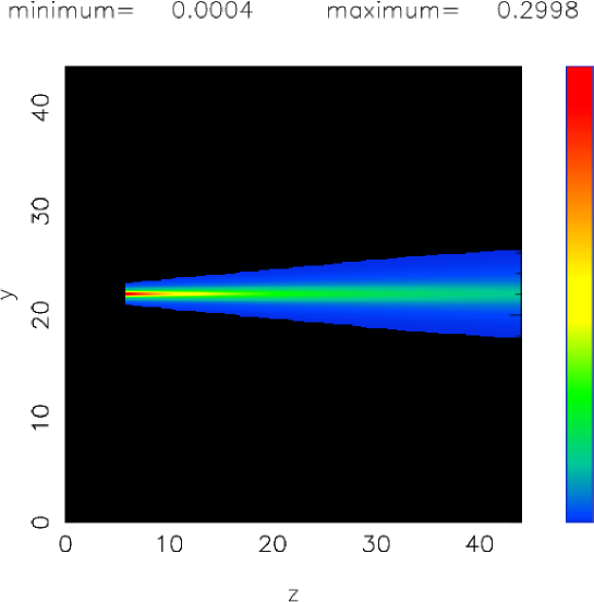
Figure 1: Theoretical 2D map of the velocity , $<U>$ , given in units of the sound speed when the initial Mach number is 0.3. The length considered is $z/d=44$ , $k$ =0.54, $A\leavevmode\nobreak\$ = 0.414 and $\alpha_{deg}=10.64$ .

The first derivative of the profile in velocity as given by formula (27) with respect to the radius is

$$\frac{d}{dr}<U>=U_{1}\times\frac{-4\,\left(\sqrt{2}-1\right){\it A\leavevmode\nobreak\ k}\,{{\it{b_{1/2}}}}^{6}A\leavevmode\nobreak\ r}{\tan\left(1/2\,\alpha\right)\left(\sqrt{2}-1\right)z\left({{\it{b_{1/2}}}}^{2}+A\leavevmode\nobreak\ {r}^{2}\right)^{3}{{\it{b_{1/2}}}}^{2}}\quad.$$ (28)

The production of turbulent kinetic energy is

$$\mathcal{P}=\nu_{T}U_{1}^{2}\times\frac{2\,\left(\sqrt{2}-1\right)^{2}{{\it A\leavevmode\nobreak\ k}}^{2}{{\it{b_{1/2}}}}^{12}{A\leavevmode\nobreak\ }^{2}{r}^{2}}{\tan\left(1/2\,\alpha\right)\left(\sqrt{2}-1\right)^{3}{z}^{2}\left({{\it{b_{1/2}}}}^{2}+A\leavevmode\nobreak\ {r}^{2}\right)^{6}{{\it{b_{1/2}}}}^{4}}\quad,$$ (29)

and $z$ should be expressed in $d$-units. It is interesting to note that the maximum of $\mathcal{P}$ , is at

$$r=\frac{1}{\sqrt{5}}\frac{b_{1/2}}{\sqrt{A\leavevmode\nobreak\ }}=0.69{b_{1/2}}\quad.$$ (30)

A quantity that is measured in the laboratory is the turbulence intensity $Tu$

$$Tu=\frac{U_{rms}}{<U>}\quad,$$ (31)

where $U_{rms}$ represents the standard deviation of the velocity measured in the laboratory and $<U>$ the averaged velocity. This quantity is $\approx$ $25\%$ at $r=0$ and rises with increasing r , see Pope (2000) and Hussein et al. (1994). Recent results obtained using the PIV (Particle Image Velocimetry) are able to produce sophisticated measurements , see Figure 2 , extracted from Bravo (2006) , who reports a 2D map of $Tu$ .

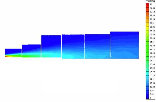
Figure 2: Laboratory map of the turbulence intensity of Nitrogen jet, Mach number=0.3. Extracted from Figure 4.18 by Bravo (2006).

A possible theoretical explanation for $Tu$ can be found from the only combination for $U_{rms}$ derived from ${\mathcal{P}}$ which produces an adimensional number when divided by ${<U>}$

$$Tu\sim\frac{\sqrt{\frac{\nu_{T}}{\rho}\frac{\partial<U>}{\partial r}}}{<U>}\quad,$$ (32)

where $\rho$ is the density. Using the practical units

$$Tu=\frac{\sqrt{2}\sqrt{{\frac{\left(\sqrt{2}-1\right){\it k}\,{{\it{b_{1/2}}}}^{4}A\leavevmode\nobreak\ r}{\rho\,z\left({{\it{b_{1/2}}}}^{2}+A\leavevmode\nobreak\ {r}^{2}\right)^{3}}}}\tan\left(1/2\,\alpha\right)z\left({{\it{b_{1/2}}}}^{2}+A\leavevmode\nobreak\ {r}^{2}\right)^{2}}{2\,\left(\sqrt{2}-1\right){\it k}\,{{\it{b_{1/2}}}}^{4}}\quad.$$ (33)

Figure 3 reports the theoretical 2D map of $Tu$ as given by equation (33) normalized to a maximum value $Tu_{max}$ as given by laboratory experiments.

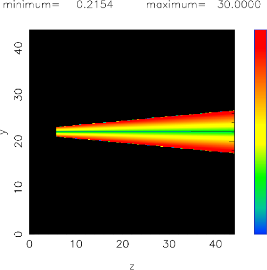
Figure 3: Theoretical 2D map of the turbulence intensity , $Tu$ , when $Tu_{max}=30\%$. The length considered is $z/d=44$ , $k$ =0.54, $A\leavevmode\nobreak\$ = 0.414 $\rho$ =1 , and $\alpha_{deg}=10.64$ .

When the flow rate of mass is expressed in these practical units equation (21) becomes

$$\dot{m(z)}=\frac{\pi\,\rho\,z\left(\tan\left(1/2\,\alpha\right)\right)^{3}{\it U_{1}}\,d}{\sqrt{2}-1}\quad.$$ (34)

In this formula both $z$ and $d$ are present and it is possible to speak of physical units, but $z\geq d$ .

0.3.2 Pipe fluids

In smooth circular tubes the averaged velocity for turbulent flow in the direction perpendicular to the motion $v_{\bot}$ is often parameterized through the following equation

$$\frac{\overline{v_{\bot}}}{v_{\bot,max}}=(1-\frac{r}{a})^{\frac{1}{n}},$$ (35)

where $r$ is the distance from the jet central axis , $a$ is the jet radius, $v_{\bot,max}$ is the maximum radial velocity and $n$ is an integer, see for example Bird et al. (2002). Figure 4 reports the mean velocity profile for different values of $n$.

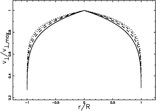
Figure 4: Mean velocity profile ( in relative units ) vs. jet radius (in relative units) when n=6 ( full line ), n=7 ( dashed ), n=8 ( dot-dash-dot-dash ), n=9 ( dotted ) and n=10( dash-dot-dot-dot ).

On introducing $\Delta R=a-r$ , the following is found:

$$\frac{\Delta R}{R}=(\frac{\overline{v_{\bot}}}{v_{\bot,max}})^{\frac{1}{n}}.$$ (36)

Further on $n$ is connected to the Reynolds number ,$Re$, through the following relationship

$$n=NINT(10^{a_{Re}}\times R^{b_{Re}}),$$ (37)

where NINT represents the nearest integer. The couple ($a_{Re},b_{Re}$) is easily found once the experimental correspondence n $\longrightarrow Re$ is provided , see for example Table 3 or  Bird et al. (2002). On applying the least square fitting procedure , $a_{Re}=$0.561 and $b_{Re}=$0.0582. Once a value of $\frac{\overline{v_{\bot}}}{v_{\bot,max}}$ is chosen we can plot $\frac{\Delta R}{R}$ as a function of the Reynolds number, see Figure 5 .

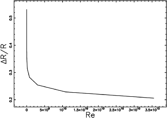
Figure 5: $\frac{\Delta R}{R}$ vs. Reynolds number when $\frac{\overline{v_{\bot}}}{v_{\bot,max}}$=0.9 .

Table 3 summarizes the equivalence between $n$, $Re$ and $\frac{\Delta R}{R}$ when $\frac{\overline{v_{\bot}}}{v_{\bot,max}}$ is fixed .

Table 3: Equivalence between parameters when $\frac{\overline{v_{\bot}}}{v_{\bot,max}}$=0.9 .

$$\begin{array}[]{ccc}\hline\cr\hline\cr\vskip 3.0pt plus 1.0pt minus 1.0pt\cr n&Re&\frac{\Delta R}{R}\\ \vskip 3.0pt plus 1.0pt minus 1.0pt\cr\hline\cr\vskip 3.0pt plus 1.0pt minus 1.0pt\cr 6&4\times 10^{3}&0.53\\ 7&1.1\times 10^{5}&0.47\\ 8&1.1\times 10^{6}&0.43\\ 9&3.2\times 10^{6}&0.38\\ \vskip 3.0pt plus 1.0pt minus 1.0pt\cr\vskip 3.0pt plus 1.0pt minus 1.0pt\cr\hline\cr\hline\cr\end{array}$$

The first derivative of the profile of perpendicular velocity as given by formula (35) is then computed

$$\frac{1}{dr}\frac{\overline{v_{\bot}}}{v_{\bot,max}}=-\frac{1}{n}(1-\frac{r}{a})^{\frac{1}{n}}\frac{1}{a-r}\quad.$$ (38)

By analogy with formula (20) a power released in the cascade as

$$\mathcal{P}_{n}=\nu_{n}(\frac{\partial v_{\bot}}{\partial r})^{2}\quad,$$ (39)

is introduced where the index $n$ stands for pipe fluid. We therefore have

$$\mathcal{P}_{n}=\frac{{\it\nu_{n}}\,\left({v_{\bot,max}}\left(-{\frac{-a+r}{a}}\right)^{{n}^{-1}}\right)^{2}}{{n}^{2}\left(-a+r\right)^{2}}\quad.$$ (40)

0.3.3 Non-Newtonian fluid

In a non-Newtonian fluid the shear stress , $\tau_{yr}$ , is often parameterized as

$$\tau_{yr}=k_{n}(-\frac{du}{dr})^{n}\quad,$$ (41)

where $k_{n}$ is a constant , $u$ the velocity , $r$ the distance from the center and $m$ an integer. The profile in velocity results to be

$$\frac{u(r)}{u_{max}}=1-(\frac{r}{a})^{\frac{m+1}{m}}\quad,$$ (42)

where $a$ is the radius of the pipe; see Problem 7-1 in The Staff of REA (1985) or Section 12.3 in Hughes & Brighton (1967). Also here we compute the first derivative of the profile of perpendicular velocity

$$\frac{d}{dr}\frac{u(r)}{u_{max}}=-\frac{\left({\frac{r}{a}}\right)^{{\frac{m+1}{m}}}\left(m+1\right)}{mr}\quad.$$ (43)

The power released in the cascade is

$$\mathcal{P}_{non}=\nu_{non}(\frac{\partial u(r)}{\partial r})^{2}\quad,$$ (44)

where the index $non$ stands for non-Newtonian fluid. We therefore have

$$\mathcal{P}_{non}=\frac{{\it\nu_{non}}\,\left(u_{max}\left({\frac{r}{a}}\right)^{{\frac{m+1}{m}}}\right)^{2}\left(m+1\right)^{2}}{{m}^{2}{r}^{2}}\quad.$$ (45)

0.4 Profiles in the perpendicular direction

The following explores how the profile in intensity of a jet intersected by a plane perpendicular to the direction of motion should appear.

Therefore, a classic Sobel filter is applied in order to find gradients in the profiles.

It is assumed that the synchrotron-emissivity scales as the power released in turbulent kinetic energy, see equation (29),

$$\epsilon\sim\mathcal{P}\quad.$$ (46)

The cross section of the jet is reported in Figure 6.

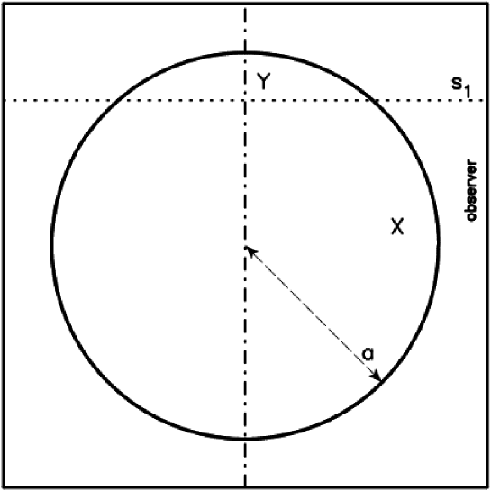
Figure 6: The conical source is represented through a section perpendicular to the jet axis. The observer is situated along the x direction, one line of sight is indicated.

Due to the additivity of the synchrotron emission along the line of sight, an integral operation is performed in order to obtain the intensity of emission

$$I(y)=\int_{0}^{\sqrt{{a}^{2}-{y}^{2}}}2\times\epsilon(r){dx}\quad,$$ (47)

with $r=\sqrt{x^{2}+y^{2}}$ and $a$ representing the jet radius.

0.4.1 Profiles of the turbulent jet

The intensity of emission according to formula (29) is

$$I(y)\sim\int_{0}^{\sqrt{{{\it a}}^{2}-{y}^{2}}}\!4\,{\frac{\left({{\it x}}^{2}+{y}^{2}\right){A\leavevmode\nobreak\ }^{2}{{\it{b_{1/2}}}}^{8}{{\it a}}^{2}}{\left({{\it{b_{1/2}}}}^{2}+A\leavevmode\nobreak\ {{\it x}}^{2}+A\leavevmode\nobreak\ {y}^{2}\right)^{6}{z}^{2}\left(\sqrt{2}-1\right)\tan\left(1/2\,\alpha\right)}}{d{\it x}}\quad.$$ (48)

This integral has an analytical solution but it is complicated and therefore Figure 7 only shows the numerical integration.

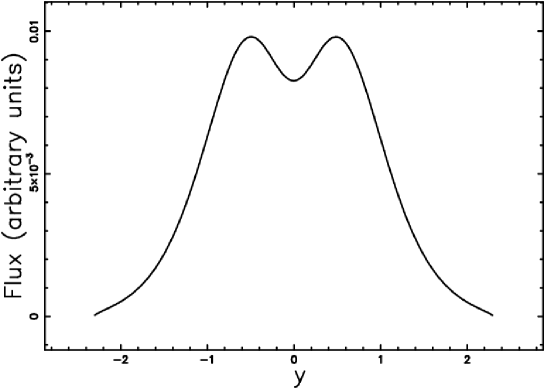
Figure 7: Intensity of radiation ${\it I(y)}$ across the turbulent jet when $z/d=44$ , $k$ =0.54, $A\leavevmode\nobreak\$ = 0.414 and $\alpha_{deg}=10.64$ .

The numerical integration gives a characteristic shape on the top of the blob which is called the ”valley on the top” and the observational counterpart of this new effect will be discussed in Section 0.4.4. The maximum of this integral is at the point $y\approx 0.49135{b_{1/2}}$ and the value of intensity at the maximum is $1.18$ times the value at the point $y=0$ ( the center of the jet).

0.4.2 Profiles of the pipe fluids

The intensity of emission in pipe fluids according to formula (40) is

$$I(y)\sim\int_{0}^{\sqrt{{a}^{2}-{y}^{2}}}\frac{{\it 2\nu_{n}}\,\left[{v_{\bot,max}}\left(-{\frac{-a+\sqrt{{x}^{2}+{y}^{2}}}{a}}\right)^{{n}^{-1}}\right]^{2}}{{n}^{2}\left(a-\sqrt{{x}^{2}+{y}^{2}}\right)^{2}}{dx}\quad.$$ (49)

The previous integral has an analytical solution in the case $n=1$

$$I(y)=2\,{\frac{{\it\nu_{n}}\,{{\it{v_{\bot,max}}}}^{2}\sqrt{{a}^{2}-{y}^{2}}}{{a}^{2}}}\quad,$$ (50)

which is reported in Figure 8.

When $n\neq 1$ the integral cannot be solved in terms of any of the standard mathematical functions

and Figure 9 reports the numerical integration .

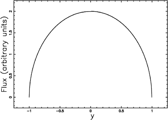
Figure 8: Intensity of radiation ${\it I(y)}$ across the pipe fluid jet, when $\nu_{n}=1$ , $a=1$ , ${v_{\bot,max}}=1$ and $n=1$ .

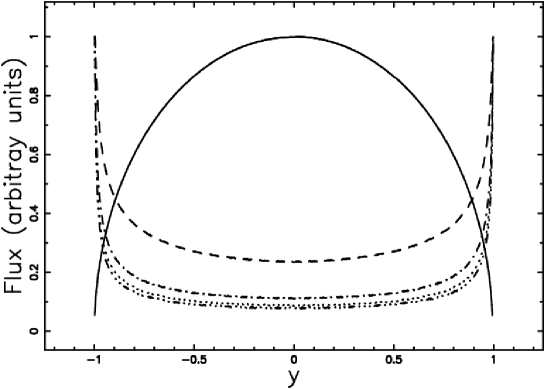
Figure 9: Intensity of radiation ${\it I(y)}$ across the pipe fluid jet normalized to 1 , when $\nu_{n}=1$ , $a=1$ , ${v_{\bot,max}}=1$ and $n=1$ (full line ), $n=2$ (dashed ), $n=3$ (dot-dash-dot-dash), $n=4$ (dotted) and $n=5$ (dash-dot-dot-dot) .

0.4.3 Profiles of non-Newtonian fluid

The intensity of emission in a non-Newtonian fluid according to formula (45) is

$$I(y)=\int_{0}^{\sqrt{{a}^{2}-{y}^{2}}}\frac{2\,{\it\nu_{non}}\,{{\it u_{max}}}^{2}\left[\left({\frac{\sqrt{{x}^{2}+{y}^{2}}}{a}}\right)^{{\frac{m+1}{m}}}\right]^{2}\left(m+1\right)^{2}}{{m}^{2}\left({x}^{2}+{y}^{2}\right)}{dx}\quad.$$ (51)

Inserting $\nu_{non}$=1 , $a=1$ and $u_{max}$=1 for the sake of simplicity, the previous integral has the analytical solution

$$I(y)=$$

$$2\,\left({y}^{2}\right)^{{\frac{m+1}{m}}}\sqrt{1-{y}^{2}}{\leavevmode\nobreak\ {}_{2}F_{1}(1/2,1-{\frac{m+1}{m}};\,3/2;\,-{\frac{1-{y}^{2}}{{y}^{2}}})}\left(m+1\right){y}^{-2}{m}^{-1}+$$

$$2\,\left({y}^{2}\right)^{{\frac{m+1}{m}}}\sqrt{1-{y}^{2}}{\leavevmode\nobreak\ {}_{2}F_{1}(1/2,1-{\frac{m+1}{m}};\,3/2;\,-{\frac{1-{y}^{2}}{{y}^{2}}})}\left(m+1\right){m}^{-2}{y}^{-2}$$ (52)

where ${\leavevmode\nobreak\ {}_{2}F_{1}(a,b;\,c;\,z)}$ is a regularized hyper-geometric function, see Abramowitz & Stegun (1965),von Seggern (1992) and Thompson (1997). Figure 10 reports the results of the numerical integration.

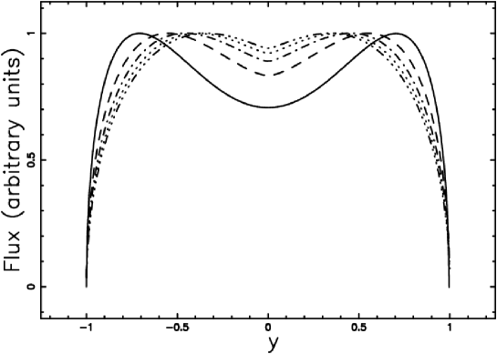
Figure 10: Intensity of radiation ${\it I(y)}$ across the non-Newtonian jet normalized to 1 when $\nu_{non}$=1 , $a=1$ and $u_{max}$=1, and $m=1$ (full line ), $m=2$ (dashed ), $m=3$ (dot-dash-dot-dash), $m=4$ (dotted) and $m=5$ (dash-dot-dot-dot) .

0.4.4 Comparison with observations

This paragraph starts by checking the profile in the direction perpendicular to the jet of M87 , in particular to the X-component of knot D-E in Figure 2 by Perlman & Wilson (2005). The data of the observations are reported in Figure 11 together with the turbulent jet profile scaled in order so that the value of half theoretical and observed intensity are approximately equal.

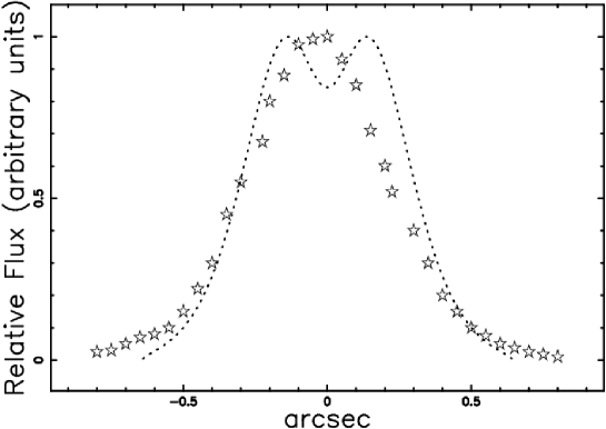
Figure 11: X-intensity of knot D-E in M87 (empty stars ) and theoretical intensity of radiation for turbulent fluids ${\it I(y)}$ (dotted line) when $z/d=44$ , $k$ =0.54, $A\leavevmode\nobreak\$ = 0.414 and $\alpha_{deg}=10.64$ .

Figures 12 and 13 report the comparison of pipe-fluid and non-Newtonian fluid respectively.

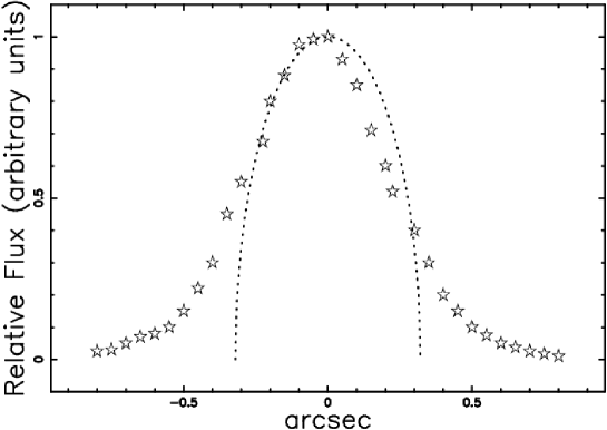
Figure 12: X-intensity of knot D-E in M87 (empty stars ) and theoretical intensity of radiation for a pipe-fluid ${\it I(y)}$ (dotted line) when $\nu_{n}=1$ , $a=1$ , ${v_{\bot,max}}=1$ and $n=1$ .

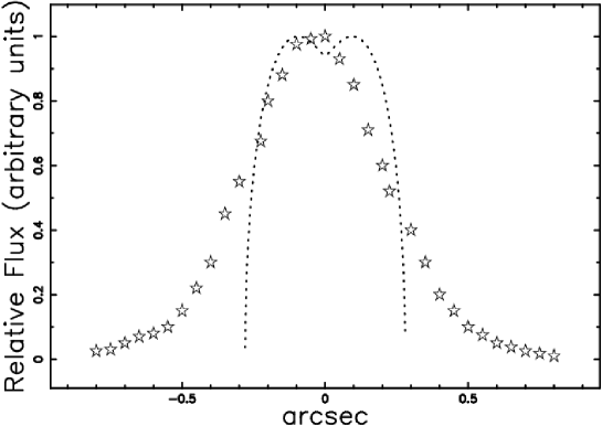
Figure 13: X-intensity of knot D-E in M87 (empty stars ) and theoretical intensity of radiation for a non non-Newtonian fluid ${\it I(y)}$ (dotted line) when $\nu_{non}$=1 , $a=1$ , $u_{max}$=1, and $m=5$ (dotted line).

Another interesting situation is represented by the four blobs in 3C273 as imaged at the frequency of 5GHz by the VSOP (VLBI ( Very Long Baseline Interferometry) Space Observatory Programme) . Here the focus is on blob A which presents a symmetry around the center of the blob and on the ”valley on the top” .

The comparison between observed and theoretical-turbulent ”valleys on the top” , see Figure 14, shows that the theoretical depression is bigger than the one observed. In the case of non-Newtonian fluid $m=5$ produces a perfect agreement between observed and theoretical depressions for blob A of 3C273, see Figure 16.

Figure 14: VSOP at the frequency of 5GHz of region A in 3C273 (empty stars ) and theoretical intensity of radiation for turbulent fluids , ${\it I(y)}$, (dotted line) when $z/d=44$ , $k$ =0.54, $A\leavevmode\nobreak\$ = 0.414 and $\alpha_{deg}=10.64$ .

0.4.5 Sobel Filter

The Sobel filter , see Pratt (1991) , computes the spatial gradient of the intensity of radio-galaxies , see , for example, Figure 4b and Figure 26b in Laing et al. (2006), which represent respectively 3C296 and 3C31. The Sobel filter is now applied in the following way . ${\bf S}$ is the the source image , ${\bf G_{x}}$ and ${\bf G_{y}}$ are the two images which at each point contain the horizontal and vertical first derivative of ${\bf S}$. At each point in the image the resulting gradient approximations can be combined to give the gradient magnitude ${\bf G}$

$${\bf G}=\sqrt{{\bf G_{x}}^{2}+{\bf G_{y}}^{2}}\quad,$$ (53)

where

$${\bf G_{x}}=\left[\begin{array}[]{ccc}1&0&-1\\ \vskip 6.0pt plus 2.0pt minus 2.0pt\cr 2&0&-2\\ \vskip 6.0pt plus 2.0pt minus 2.0pt\cr 1&0&-1\end{array}\right]\ast{\bf S}$$ (54)

and

$${\bf G_{y}}=\left[\begin{array}[]{ccc}1&2&1\\ \vskip 6.0pt plus 2.0pt minus 2.0pt\cr 0&0&0\\ \vskip 6.0pt plus 2.0pt minus 2.0pt\cr-1&-2&-1\end{array}\right]\ast{\bf S}$$ (55)

where $\ast$ denotes the 2-dimensional convolution operation. The gradient direction, $\Theta$ , is

$$\Theta=\arctan\left(\frac{{\bf G_{y}}}{{\bf G_{x}}}\right)\quad.$$ (56)

Here we have implemented the Sobel filter to 1D cuts in intensity of 3C273; Figure 15 reports the theoretical and the observed Sobel filter.

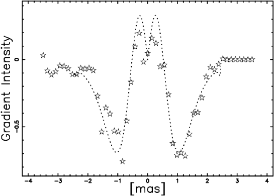
Figure 15: Gradient of the intensity (Sobel filter) for VSOP-data at the frequency of 5GHz of region A in 3C273 (empty stars ) and gradient of theoretical intensity (Sobel filter) of radiation for turbulent fluids (dotted line ). Parameters as in Figure 14.

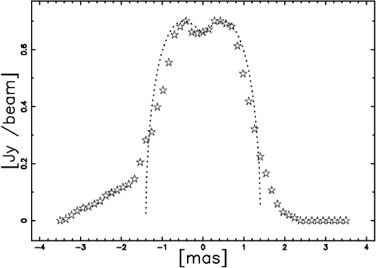
Figure 16: VSOP at the frequency of 5GHz of region A in 3C273 (empty stars ) and theoretical intensity of radiation for a non non-Newtonian fluid ${\it I(y)}$ (dotted line) when $\nu_{non}$=1 , $a=1$ , $u_{max}$=1 , and $m=5$ (dotted line).

0.5 2D maps

An algorithm is now built , which is able to simulate the synchrotron emission of the jet given the basic assumption that the emissivity $\epsilon$ scales as the power released in turbulence for a turbulent fluid. The integral operation that gives the intensity on a plane is performed through a simple addition as given by formula (15). The simplest case , a jet perpendicular to the line of sight is now analyzed.

The symmetry here used is that the jet’s main direction is perpendicular to the observer, see Figure 17.

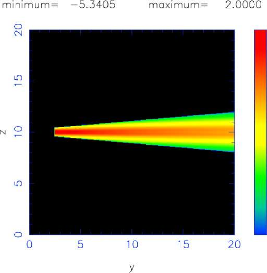
Figure 17: Theoretical 2D map of the decimal logarithm of the intensity of emission over the astrophysical length of 20$kpc$ corresponding to the radio-galaxy NGC4061 at 21 cm , see Figure 5 in Zaninetti (2007) . The length expressed in the nozzle’s diameter units is $z/d=44$ , $k$ =0.54, $A\leavevmode\nobreak\$ = 0.414 and $\alpha_{deg}=10.64$ . The integral operation is performed on a cubic grid of $400^{3}$ pixels.

In order to clarify the interpretation of this theoretical 2D color map Figure 18 reports the intensity profile along the main direction and the transversal profile as computed in the middle of the jet is shown in Figure 19.

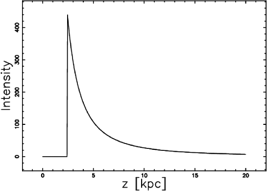
Figure 18: Cut of the intensity of emission along the main direction at the center of the jet as extracted from Figure 17 .

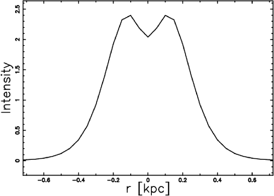
Figure 19: Cut of the intensity of emission in the transversal direction , or $90^{\circ}$ in the middle of the jet as extracted from Figure 17 .

The previous case represents a cut along a direction that forms an angle of $90^{\circ}$ with respect to the jet’s main direction. When the angles are different, the ” valley on the top” becomes asymmetric and the thickness of the cut increases , see Figure 20 where two profiles are reported.

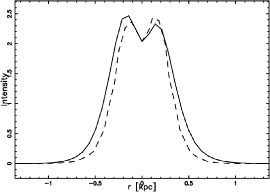
Figure 20: Cut of the intensity of emission in the middle of the jet at $45^{\circ}$ (full line) and at $120^{\circ}$ (dashed line) as extracted from Figure 17 .

The gradient magnitude of the previous image is now plotted , see Figure 21.

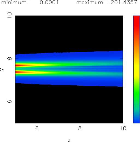
Figure 21: Sobel filter of the intensity of the central part of NGC4061. The gradient magnitude is computed according to formula (53), other parameters as in Figure 17.

0.6 Astrophysical applications

The following reports the velocity , the equation of motion , the power released in turbulence and the flow rate of mass when the astrophysical units are adopted. The algorithm that allows us to build complex trajectories such as NGC6041 and 3C31 is then introduced. The observed spectral index typical of the radio-galaxies is simulated.

0.6.1 Astrophysical equations

Here shown is the astrophysical version of the previous derived equations for the turbulent jet. Equation (16) allows us to deduce the centerline velocity

$$u_{0}(z)=162027\,{\frac{\beta_{0}\,{\it d_{1}}}{\tan\left(0.00872\,{\it\alpha_{deg}}\right)z_{1}}}\frac{Km}{sec}\quad,$$ (57)

where $\alpha_{deg}$ is the opening angle expressed in degrees, $\beta_{0}$ is the initial velocity divided by the light velocity, $d_{1}$ is the diameter of the nozzle in $kpc$ units and $z_{1}$ is the length of the jet in $kpc$ units. From the previous equation it is possible to deduce the equation of motion for a turbulent jet ,

$$z(t)=57.56\,\sqrt{{\frac{\beta_{0}\,{\it d_{1}}\,{\it t_{7}}}{\tan\left(0.00872\,{\it\alpha_{deg}}\right)}}}kpc\quad,$$ (58)

where $t_{7}$ = $t/(10^{7})$ year. The radius of the turbulent jet is

$$r(z)=[\frac{d_{1}}{2}+z(t)\tan(\frac{\alpha}{2})]kpc\quad,$$ (59)

where $\alpha$ is the opening angle expressed in radians. The power released in the turbulent cascade is

$$\epsilon(r,z)=\frac{2\,\left(\sqrt{2}-1\right)^{2}{{\it k}}^{2}{{\it b_{1/2}}}^{12}{A\leavevmode\nobreak\ }^{2}{r}^{2}}{\tan\left(1/2\,\alpha\right)\left(\sqrt{2}-1\right)^{3}\left({{\it b_{1/2}}}^{2}+A\leavevmode\nobreak\ {r}^{2}\right)^{6}{{\it b_{1/2}}}^{4}}(\frac{d_{1}}{z_{1}})^{2}\quad,$$ (60)

where $z_{1}$ is the position of the jet expressed in $kpc$ units , $A$ and $k$ are defined in Section 0.3.1 .

The flow rate of mass , see equation (34) , as expressed in these astrophysical units is

$$\dot{m}(z)=8.0\,10^{11}{\it n_{0}}\,{\it z_{1}}\,\left[\tan\left(\frac{\alpha}{2}\right)\right]^{3}\beta_{0}\,{\it d_{1}}\,\frac{{\mathcal{M}}_{\sun}}{10^{7}\mbox{year}}\quad,$$ (61)

where $\rho_{0}=n_{0}m$ , $m=1.4\leavevmode\nobreak\ m_{\mathrm{H}}$ , $n_{0}$ is the density expressed in particles $\mathrm{cm}^{-3}$ , $m_{\mathrm{H}}$ is the mass of the Hydrogen and ${\mathcal{M}}_{\sun}$ is the mass of the Sun.

0.6.2 Astrophysical images

The points belonging to a trajectory , in the following TP , are now inserted on a cubic lattice made by $pixels^{3}$ points . The intensity in each point of a 2D grid is computed according to the following rules.

1. In each point of a 3D grid we compute the nearest TP.

2. The concentration on a 3D grid is then computed because we know the distance between the grid point and the nearest TP.

3. The intensity of radiation is then computed according to the integral operation as represented by formula (15).

A first test can be done on a radio galaxy already examined in Zaninetti (2007), NGC4061. The equation of motion is formula (58), derived in the previous paragraph. The other parameters necessary to produce bending and wiggling of the jet as well as the Eulerian angles which represent the point of view are reported in the caption of Figure 22.

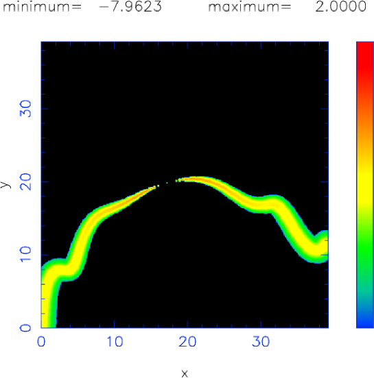
Figure 22: Theoretical 2D map of the decimal logarithm of the intensity of emission representing the continuous three-dimensional trajectory of NGC4061: the three Eulerian angles characterizing the point of view are $\Phi$=80 ^∘ , $\Theta$=-85 ^∘ and $\Psi$=-10 ^∘. The precession is characterized by the angle $\Psi_{prec}$= 5 ^∘ and by the angular velocity $\Omega_{prec}$= 60.00 [${}^{\circ}/10^{7}\mathrm{year}$]. The three Eulerian angles which characterize the jet are $\Phi_{j}$= 0 ^∘ , $\Psi_{j}$= 0 ^∘ and $\Theta_{j}$= 90 ^∘. The angle of rotation of the galaxy is $\alpha_{G}$= 0 ^∘. The physical parameters characterizing the jet motion are : $t_{7}$= 12.00 $10^{7}\mathrm{year}$, $d_{1}$= 0.01 ${\mathrm{kpc}}$ , $\beta_{0}$ = 0.1 , $\alpha_{0}$= 10.64 ^∘. The length of the jet is 20.6 ${\mathrm{kpc}}$ and the velocity of the galaxy $v_{z}$= 117 ${\mathrm{km/s}}$ . The integral operation is performed on cubic grid of $500^{3}$ pixels.

The phenomena of the ”valley on the top” can be visualized through a surface rendering of the 2D intensity , see Figure 23 , or through a 1D cut of the matrix that represents the intensity , see Figure 24 .

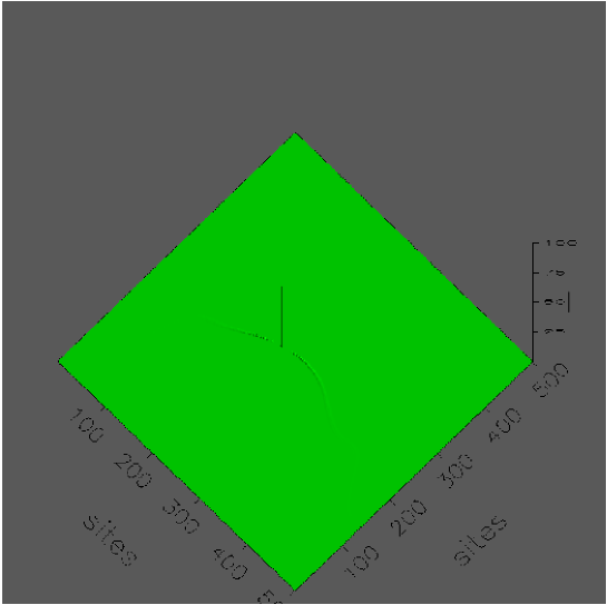
Figure 23: Intensity of NGC4061 represented through a surface , parameters as in Figure 22. The observer sees the surface at an angle of 70^∘.

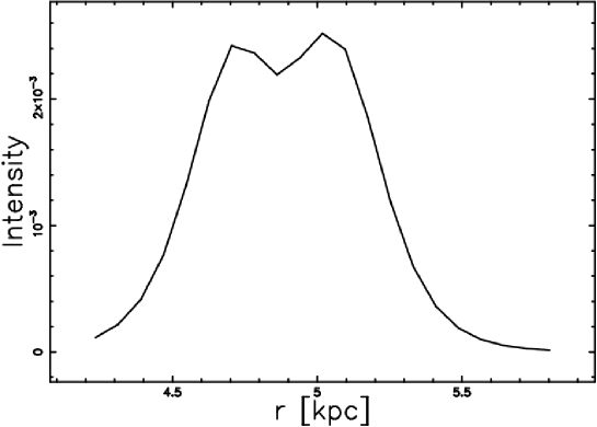
Figure 24: Intensity of NGC4061 represented through a cut in the x-direction , parameters as in Figure 22.

Another radio-galaxy that can be here simulated is 3C31 ; this radio-galaxy has been chosen because it does not present knots, see radio observations in Figure 25. This radio-galaxy has already been simulated in the first straight 12 $kpc$ , and a comparison between the model and the observed brightness distribution is reported in Figure 6 of Laing & Bridle (2002b) and in Figure 3 of Laing et al. (2005) . The first 60 $kpc$ are simulated in order to cover the wiggles. The 3D surface that represents the trajectory is presented in Figure 26, the simulated intensity distribution is reported in Figure 27 , Figure 28 reports the gradient magnitude computed according to the Sobel filter, Figure 29 reports the intensity represented through a surface rendering that visualizes the ”valley on the top”, and Figure 30 reports the intensity represented through a 1D cut.

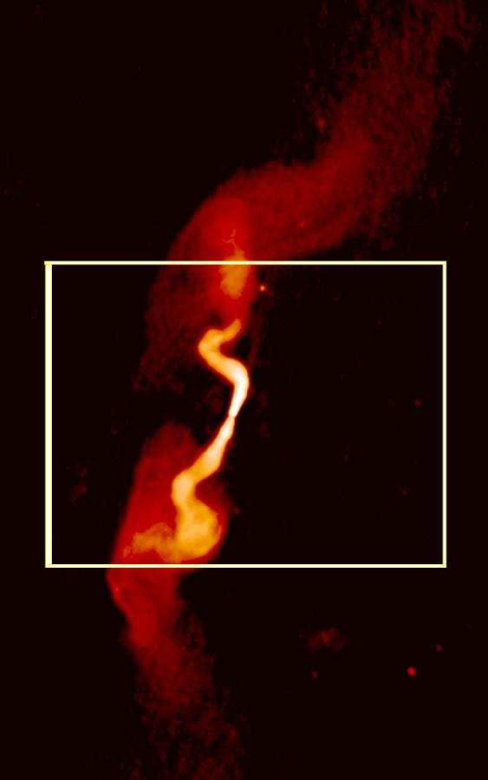
Figure 25: The large scale structure of 3C31 at the frequency of 1.4 GHz. The north-south field covers 300 $kpc$ and the small box here modeled covers 120 $kpc$. This image was generated with data from telescopes of the National Radio Astronomy Observatory, a National Science Foundation Facility, managed by Associated Universities. Inc .

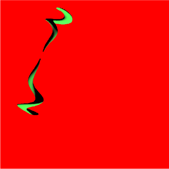
Figure 26: Continuous three-dimensional surface of 3C31: the three Eulerian angles characterizing the point of view are $\Phi$=180 ^∘ , $\Theta$=170 ^∘ and $\Psi$=195 ^∘. The precession is characterized by the angle $\Psi_{prec}$= 10 ^∘ and by the angular velocity $\Omega_{prec}$= 54.00 [${}^{\circ}/10^{7}\mathrm{year}$]. The three Eulerian angles which characterize the jet are $\Phi_{j}$= 0 ^∘ , $\Psi_{j}$= 0 ^∘ and $\Theta_{j}$= 90 ^∘. The angle of rotation of the galaxy is $\alpha_{G}$= 0 ^∘. The physical parameters characterizing the jet motion are : $t_{7}$= 10.00 $10^{7}\mathrm{year}$, $d_{1}$= 0.2 ${\mathrm{kpc}}$ , $\beta_{0}$ = 0.05 , $\alpha_{0}$= 10.64 ^∘. The length of the jet is 59.65 ${\mathrm{kpc}}$ and the velocity of the galaxy $v_{z}$= 292 ${\mathrm{km/s}}$ .

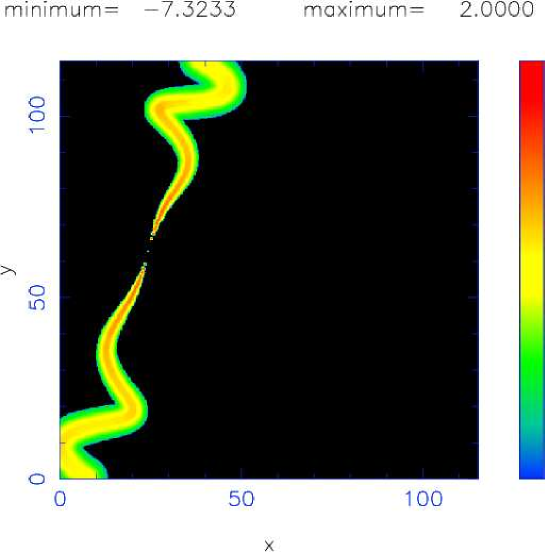
Figure 27: Theoretical 2D map of the decimal logarithm of the intensity of emission representing the continuous three-dimensional trajectory of 3C31; parameters as in Figure 26 . The integral operation is performed on a cubic grid of $500^{3}$ pixels.

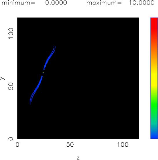
Figure 28: Sobel filter of the intensity of the central part of 3C31. The gradient magnitude is computed according to formula (53), parameters as in Figure 26 .

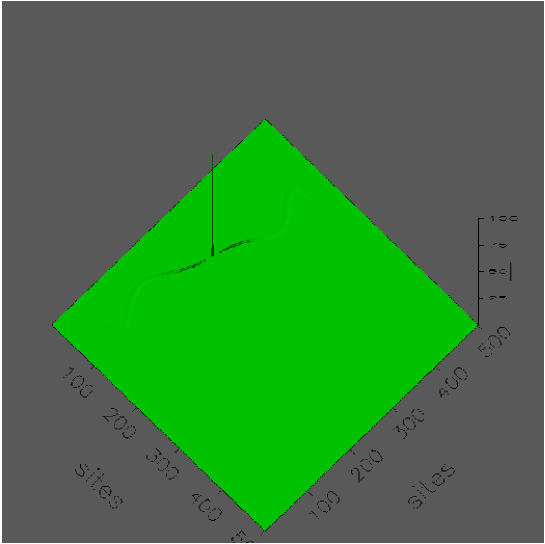
Figure 29: Intensity of 3C31 represented through a surface , parameters as in Figure 26 and Figure 27. The observer sees the surface at an angle of 70^∘.

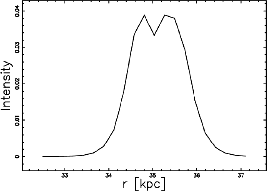
Figure 30: Intensity of 3C31 represented through a 1D cut along the x-direction , parameters as in Figure 26 and Figure 27.

0.6.3 Spectral index

The collision of an electron of energy $E$ with a cloud produces an average gain in energy ($\Delta E$) proportional to the second order in $u/c$ , $u$ is cloud velocity and $c$ is light velocity,

$$\langle\frac{\Delta E}{E}\rangle=\frac{8}{3}(\frac{u}{c})^{2}\quad.$$ (62)

This process is named Fermi II after Fermi (1949).

On introducing an average length of collision , $\lambda$ , the formula becomes:

$$\frac{dE}{dt}=\frac{E}{\tau}\quad,$$ (63)

where

$$\tau=\frac{4}{3}(\frac{u^{2}}{c^{2}})(\frac{c}{\lambda})\quad.$$ (64)

It should be remembered that with a mean free path between clouds $\lambda$, the average time between collisions with clouds , see Lang (1999) , is

$$2\frac{\lambda}{c}\quad.$$ (65)

The probability , $P(t)$ , of the particle remaining in the reservoir for a period greater than $t$ is,

$$P(t)=e^{-\frac{t}{T}}\quad,$$ (66)

where $T$ is the time of escape from the considered region. The hypothesis that energy is continuously injected in the form of relativistic particles with energy $E_{0}$ at the rate R, produces ( according to Burn (1975)) the following probability density , $N$ , which is a function of the energy:

$$N(E)=\frac{R\tau}{E_{0}}\left(\frac{E}{E_{0}}\right)^{-\gamma}\quad,$$ (67)

with

$$\gamma=1+\frac{\tau}{T}\quad,$$ (68)

and $\tau$ is defined in equation (64) . Equation (67) can be written as

$$N(E)=K\;E^{-\gamma}\quad,$$ (69)

where $K=\frac{R\tau}{{E_{0}}^{-\gamma+1}}$ . A power law spectrum in the electron energy has now been obtained. A power law distribution of relativistic electrons ,see Lang (1999) , corresponds to a power law frequency spectrum proportional to $\nu^{\alpha_{s}}$ , where the spectral index $\alpha_{s}$ is

$$\alpha_{s}=-\frac{\gamma-1}{2}=-\frac{\tau}{2T}\quad.$$ (70)

$T$ is now assumed to be constant and $\tau$ scales with the power released in turbulent kinetic energy, $\epsilon$ , as

$$\tau\approx\frac{1}{[\epsilon(r,z)]^{1/b}}\quad,$$ (71)

where $b$ is a parameter that connects theory with observations. Concerning the observations of the spectral index along the jet we concentrate on 3C273 , see X-observations by Jester et al. (2006) and far-ultraviolet imaging by Jester et al. (2007). Table 3 in X-Ray by Jester et al. (2006) was selected as an example to simulate : the spectral index is 0.83 at knot $B1$ (internal region) and 1.27 at knot $H2$ (external region). Therefore as suggested by the theoretical formula (70) the observed spectral index increases in absolute value going from the inner regions to the outer regions. The theoretical spectral index was simulated in the following way

1. A spectral index is generated according to formula (70) in each point of the 3D jet. A typical 2D cut is reported in Figure 31.

2. The intensity at the frequency $\nu$, $I_{\nu}$ , is computed in each point of the jet according to equation (60).

3. The intensity at a frequency one decade bigger , $\nu\times 10$, is evaluated according to the scaling , $I_{\nu\times 10}=I_{\nu}(10)^{\alpha_{s}}$ .

4. The integral operation is performed on a cubic grid of $pixels^{3}$ points. The spectral index that comes from the two integral operations at two different frequencies is computed , see Figure 32. The parameter $b$ is chosen in order to fit the observations.

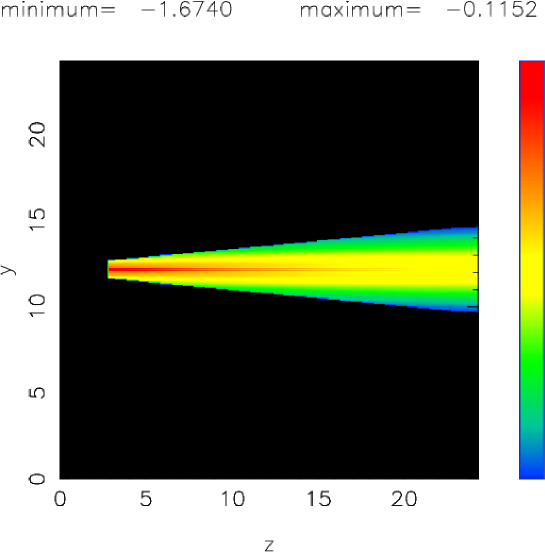
Figure 31: Cut of the first spectral index through a plane crossing the center of the jet, $b$=14. The length of the jet is $24kpc$ , the same as 3C273. The 2D grid is made of $400^{2}$ pixels.

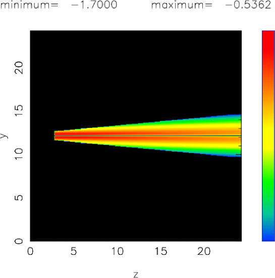
Figure 32: Spectral index of 3C373 as comes from the integral operation over two frequencies. The integral operation is performed on cubic grid of $400^{3}$ pixels.

In this simulation , see Figure 32 , the spectral index increases in absolute value both in going from the internal regions to the external regions following the axial direction and in going from the center of the jet to the boundary along the perpendicular direction. This effect has been observationally mapped in the case of 3C296 , see for example Figure 4b in Laing et al. (2006) .

Under the hypothesis of ultra-relativistic electrons , a power law $-\gamma$ in the energy distribution of the electrons and a uniform magnetic field, the degree of linear polarization is, see equation (1.176) in Lang (1999) ,

$$\prod=\frac{\gamma+1}{\gamma+7/3}\quad.$$ (72)

Figure 33 maps the degree of linear polarization that comes from the 2D map of the spectral index after a conversion of the index $\gamma$ in $\alpha_{s}$ ,

$$\prod=\frac{3(1-\alpha_{s})}{3\alpha_{s}-5}\quad.$$ (73)

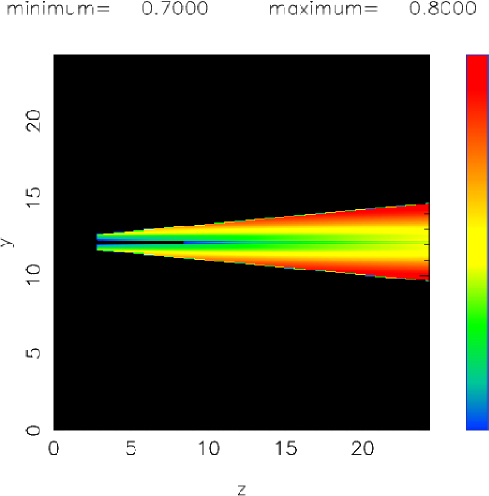
Figure 33: Degree of linear polarization of 3C373; parameters as in Figure 32 .

0.7 Summary

Theoretical Emissivity  The power released in the turbulence is computed for three type of fluids. The maximum input in turbulence is realized when $r=0.69{b_{1/2}}$ , in the case that turbulent fluids are considered.

Theoretical Intensity Profiles  The profiles in intensity of synchrotron radiation perpendicular to the line of sight are analytically or numerically solved when the simplest configuration is realized : straight jets oriented in the direction perpendicular to the observer. The maximum of synchrotron radiation for turbulent fluids is at $r\approx 0.49{b_{1/2}}$. This means that a depression at the center of the jet is expected. The three types of synchrotron radiation here analyzed are then compared with the observed X-component of knot D-E in M87 and with knot A in 3C273 at the frequency of 5GHz. The confrontation with the data from astronomical observations should be carefully done because the data are often smoothed and this operation may change the structure of the central depression.

Theoretical Radio maps More complex is the set up of an algorithm that implements the radiative transfer equation for a randomly oriented jet. In order to build such an image, the centerline trajectory should be made discrete and the distance between the point of a 3D grid and the nearest point of the trajectory computed. This algorithm computes the theoretical map in intensity of synchrotron radiation for complex morphological cases such as NGC4061. The depression at the center of the jet , Figure 23, can be considered an alternative to the cosmic double helix , see Lobanov & Zensus (2001); Lobanov et al. (2005).

Theoretical Spectral Index The connection between power released in turbulence and acceleration of electrons has been attached adopting a Fermi mechanism with a variable velocity of acceleration. This mechanism, after the introduction of a parameter that connects theory and observations allows us to build 2D maps of the theoretical spectral index of synchrotron emission, see Figure 32. The simulation predicts that the spectral index should decrease ( it increases in absolute value) along the centerline and the transversal directions. As a consequence the 2D map of the degree of linear polarization is easily built.

Theoretical Sobel Filter The new technique of the Sobel Filter can detect details in the map of radio-galaxies. The phenomena of the ”valley on the top” can be revealed due to the gradient’s change of sign in going from the center to the external regions in a radial direction, see Figure 15 and Figure 21 . The presence of arcs in the Sobel-filtered images , see Figure 26b in Laing et al. (2006) , can be explained by the fact that the integral operation that leads to the intensity of radio-galaxies is made in presence of curved zones of emission.

I express my gratitude to Miguel Onorato for useful help during the set up of Figure 2.

References

- Abramowitz & Stegun (1965) Abramowitz, M. & Stegun, I. A. 1965, Handbook of mathematical functions with formulas, graphs, and mathematical tables (New York: Dover)
- Bicknell (1984) Bicknell, G. V. 1984, ApJ , 286, 68
- Bird et al. (2002) Bird, R., Stewart, W., & Lightfoot, E. 2002, Transport Phenomena ; second Edition (New York: John Wiley and Sons)
- Bravo (2006) Bravo, L. 2006, Ph.D. thesis, The City University of New York
- Bridle et al. (1980) Bridle, A. H., Henriksen, R. N., Chan, K. L., Fomalont, E. B., Willis, A. G., & Perley, R. A. 1980, ApJ , 241, L145
- Burn (1975) Burn, B. J. 1975, A&A , 45, 435
- Canvin & Laing (2004) Canvin, J. R. & Laing, R. A. 2004, MNRAS , 350, 1342
- Eilek et al. (2003) Eilek, J., Hardee, P., & Lobanov, A. 2003, New Astronomy Review, 47, 505
- Falle (1994) Falle, S. A. E. G. 1994, MNRAS , 269, 607
- Favre (1969) Favre , A. 1969, Problems of hydrodynamics and continuum mechanics (Philadelphia: Society for Industrial and Applied Mathematics)
- Fermi (1949) Fermi, E. 1949, Physical Review, 75, 1169
- Ferrari et al. (1979) Ferrari, A., Trussoni, E., & Zaninetti, L. 1979, A&A , 79, 190
- Ginsburg (1975) Ginsburg, V. 1975, Physique Teorique et Astrophysique (Moscou: Editions MIR)
- Hughes & Brighton (1967) Hughes, W. & Brighton, J. 1967, Fluid Dynamics (New York: McGraw-Hill)
- Hussein et al. (1994) Hussein, H. J., Capp, S. P., & George, W. K. 1994, Journal of Fluid Mechanics, 258, 31
- Jester et al. (2006) Jester, S., Harris, D. E., Marshall, H. L., & Meisenheimer, K. 2006, ApJ , 648, 900
- Jester et al. (2007) Jester, S., Meisenheimer, K., Martel, A. R., Perlman, E. S., & Sparks, W. B. 2007, MNRAS , 380, 828
- Kundt (1979) Kundt, W. 1979, Astrophysics and Space Science, 62, 335
- Kundt (2006) —. 2006, Chinese Journal of Astronomy and Astrophysics Supplement, 6, 279
- Kundt & Gopal Krishna (2004) Kundt, W. & Gopal Krishna. 2004, J. Astrophys. Astr., 25, 115
- Laing & Bridle (2002a) Laing, R. A. & Bridle, A. H. 2002a, MNRAS , 336, 328
- Laing & Bridle (2002b) —. 2002b, MNRAS , 336, 328
- Laing et al. (2005) Laing, R. A., Canvin, J. R., & Bridle, A. H. 2005, in X-Ray and Radio Connections (eds. L.O. Sjouwerman and K.K Dyer) Published electronically by NRAO, http://www.aoc.nrao.edu/events/xraydio Held 3-6 February 2004 in Santa Fe, New Mexico, USA, (E7.02) 14 pages
- Laing et al. (2006) Laing, R. A., Canvin, J. R., Bridle, A. H., & Hardcastle, M. J. 2006, MNRAS , 372, 510
- Lang (1999) Lang, K. R. 1999, Astrophysical formulae. (Third Edition) (New York: Springer)
- Lobanov et al. (2005) Lobanov, A., Hardee, P., & Eilek, J. in , Astronomical Society of the Pacific Conference Series, Vol. 340, Future Directions in High Resolution Astronomy, ed. J. RomneyM. Reid, 104–+
- Lobanov & Zensus (2001) Lobanov, A. P. & Zensus, J. A. 2001, Science, 294, 128
- Nishikawa et al. (2006) Nishikawa, K.-I., Hardee, P. E., Hededal, C. B., & Fishman, G. J. 2006, ApJ , 642, 1267
- Noriega-Crespo et al. (1996) Noriega-Crespo, A., Garnavich, P. M., Raga, A. C., Canto, J., & Boehm, K.-H. 1996, ApJ , 462, 804
- Pelletier & Zaninetti (1984) Pelletier, G. & Zaninetti, L. 1984, A&A , 136, 313
- Perlman & Wilson (2005) Perlman, E. S. & Wilson, A. S. 2005, ApJ , 627, 140
- Pope (2000) Pope, S. B. 2000, Turbulent Flows (Cambridge, UK: Cambridge University Press)
- Pratt (1991) Pratt, W. 1991, Digital Image Processing (New York: Wiley)
- Rybicki & Lightman (1985) Rybicki, G. & Lightman, A. 1985, Radiative Processes in Astrophysics (New-York: Wiley-Interscience)
- Schlichting et al. (2004) Schlichting, H., Gersten, K., Krause, E., & Oertel, H. J. 2004, Boundary-Layer Theory (New-York: Springer)
- The Staff of REA (1985) The Staff of REA , . 1985, Transport Phenomena Problem Solver (Piscataway: Research and Education Association)
- Thompson (1997) Thompson, W. J. 1997, Atlas for computing mathematical functions (New York: Wiley-Interscience)
- von Seggern (1992) von Seggern, D. 1992, CRC Standard Curves and Surfaces (New York: CRC)
- Worrall et al. (2007) Worrall, D. M., Birkinshaw, M., Laing, R. A., Cotton, W. D., & Bridle, A. H. 2007, MNRAS , 380, 2
- Zaninetti (1989) Zaninetti, L. 1989, A&A , 223, 369
- Zaninetti (1999) —. 1999, Journal of Computational Physics, 156, 382
- Zaninetti (2007) —. 2007, Revista Mexicana de Astronomia y Astrofisica, 43, 59