Incommensurate Antiferromagnetism Coexisting with Superconductivity in Two-Dimensional d-p Model

Abstract

Numerical studies of the two-dimensional d-p model using the Gutzwiller ansatz have exhibited the incommensurate antiferromagnetic state coexisting with superconductivity in the under- and lightly doped regions. Our results are based on the variational Monte Carlo method for the three-band Hubbard model with d and p orbitals. We obtained the finite superconducting condensation energy for the coexistent sate at the doping rate $x=1/8$, 1/12, and 1/16, up to the systems of 256 unit cells with 768 atoms (oxygen and copper atoms). The phase diagram for the hole-doped case is consistent with recent results reported for layered high temperature cuprates.

The mechanisms of superconductivity (SC) in high-temperature superconductors have been extensively studied using various two-dimensional (2D) models of electronic interactionsdag94 ; ben03 ; and97 ; mor00 . It is of primary importance to clarify the phase diagram, particularly the electronic state in the underdoped region adjacent to the antiferromagnetic (AF) phase, termed the pseudo-gap phase. It is unclear whether the phase diagram for La_2-xSr_xCuO₄ is intrinsic for high-$T_{c}$ cuprates or not, although it is often recognized as a typical phase diagram. It is sometimes declared that disorder effects play some role in the spin glass phase of La_2-xSr_xCuO₄. Thus, it is fair to say that the phase diagram has never been clarified.

The 2D three-band d-p model is the most fundamental model for high-temperature cuprateshir89 ; sca91 ; tak97 ; gue98 ; kob98 ; koi00 ; yan01 . Although we have a solution of the gap equation within a weak coupling perturbation theory in the limit $U\rightarrow 0$koi01 ; yan08 , it is, however, extremely hard to show the possibility of superconductivity exactly for finite and large Coulomb repulsion. Thus we adopt the Gutzwiller ansatz for the wave function and examine the ground state within the space of variational functions. We employ the variational Monte Carlo methodgro87 ; yok87 ; nak97 ; yam98 to evaluate the expectation values of several physical properties.

The purpose of this study is to investigate the coexistence of superconductivity and antiferromagnetism for the 2D d-p model. We have found that the coexistent state has indeed the lowest energy in the variational space at the doping rate $x=0.125$, 0.08333, and 0.0625 in the low-doping region. At $x=0.125$, the incommensurate antiferromagnetic state has eight-lattice periodicity, as reported on the basis of neutron scattering measurementstra96 . The periodicity increases as $x$ decreases; we have twelve lattice periodicity at $x=0.0833$ and sixteen-lattice periodicity at $x=0.0625$.

The Hamiltonian is the d-p model containing the on-site Coulomb repulsion for d electrons and is written aseme87

$$H_{dp} = \epsilon_{d}\sum_{i\sigma}d_{i\sigma}^{{\dagger}}d_{i\sigma}+\epsilon_{p}\sum_{i\sigma}(p_{i+\hat{x}/2\sigma}^{{\dagger}}p_{i+\hat{x}/2\sigma}$$ (1)

$$+ p_{i+\hat{y}/2\sigma}^{{\dagger}}p_{i+\hat{y}/2\sigma})$$

$$+ t_{dp}\sum_{i\sigma}[d_{i\sigma}^{{\dagger}}(p_{i+\hat{x}/2\sigma}+p_{i+\hat{y}/2\sigma}-p_{i-\hat{x}/2\sigma}-p_{i-\hat{y}/2\sigma})$$

$$+ {\rm h.c.}]+t_{pp}\sum_{i\sigma}[p_{i+\hat{y}/2\sigma}^{{\dagger}}p_{i+\hat{x}/2\sigma}-p_{i+\hat{y}/2\sigma}^{{\dagger}}p_{i-\hat{x}/2\sigma}$$

$$- p_{i-\hat{y}/2\sigma}^{{\dagger}}p_{i+\hat{x}/2\sigma}+p_{i-\hat{y}/2\sigma}^{{\dagger}}p_{i-\hat{x}/2\sigma}+{\rm h.c.}]$$

$$+ U_{d}\sum_{i}d_{i\uparrow}^{{\dagger}}d_{i\uparrow}d_{i\downarrow}^{{\dagger}}d_{i\downarrow}.$$

$d_{i\sigma}$ and $d^{{\dagger}}_{i\sigma}$ are the operators for the $d$ electrons. $p_{i\pm\hat{x}/2\sigma}$ and $p^{{\dagger}}_{i\pm\hat{x}/2\sigma}$ denote the operators for the $p$ electrons at the site $R_{i\pm\hat{x}/2}$, and in a similar way, $p_{i\pm\hat{y}/2\sigma}$ and $p^{{\dagger}}_{i\pm\hat{y}/2\sigma}$ are defined. $U_{d}$ is the strength of the on-site Coulomb energy between $d$ electrons. The number of sites is denoted as $N_{s}$, and the total number of atoms is $N_{a}=3N_{s}$. The total number of fermions is denoted as $N_{e}$. The energy unit is given by $t_{dp}$ in this paper.

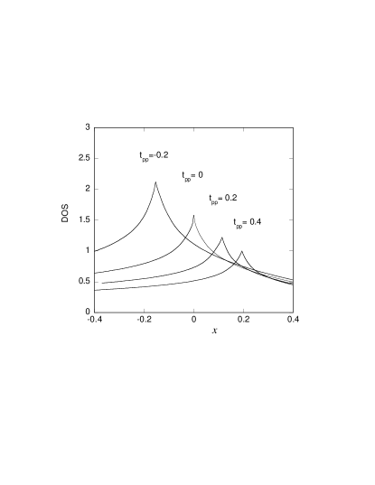
Figure 1: Density of states of the d-p model as a function of the carrier density $x$ for $t_{pp}=0.4$, 0.2, 0.0 and -0.2. We set $\epsilon_{p}=0$, $\epsilon_{d}=-1$ and $t_{dp}=1$ (energy unit).

The van Hove singularity in the density of states plays an important role in two-dimensional models. We define the density of states as

$$D(\epsilon)=\frac{1}{N_{s}}\sum_{{\bf k}}\delta(\epsilon-\xi_{{\bf k}}),$$ (2)

where $\xi_{{\bf k}}=\epsilon_{{\bf k}}-\mu$ ($\mu$ is the Fermi energy) and $\epsilon_{{\bf k}}$ is the band crossing the Fermi energy. We examine the hole-doped case within the hole picture where the lowest band is occupied up to the Fermi energy $\mu$. For this purpose, we employ the electron-hole transformation $t_{pp}\rightarrow-t_{pp}$, $t_{dp}\rightarrow-t_{dp}$, and we set $\epsilon_{p}-\epsilon_{d}>0$. The density of states $D(\epsilon)$ as a function of the carrier density $x$ is shown in Fig. 1 for $t_{pp}=0.4$, 0.2, 0, and -0.2. $x=0$ corresponds to the half-filled band. For $t_{pp}=0$, the van Hove singularity is at $x=0$. It moves to the hole-doped side of $x>0$ for $t_{pp}>0$ and to the electron-doped side for $t_{pp}<0$. We have the van Hove singularity at $x\sim 0.16$ for $\epsilon_{p}-\epsilon_{d}=2$ and $t_{pp}=0.4$. Thus we set parameters to be $\epsilon_{p}-\epsilon_{d}=2$ and $t_{pp}=0.4$ in the main computations, and $U_{d}=8$ in this paper. This is in good accordance with the results of cluster estimationsesk89 ; hyb90 ; mcm90 . The van Hove singularity approaches $x=0$ as the level difference $\epsilon_{p}-\epsilon_{d}$ becomes large. Hence, we expect that the critical temperature $T_{c}$ has a peak as a function of $\epsilon_{p}-\epsilon_{d}$ if we fix the carrier density $x$.

We adopt the Gutzwiller ansatz for the ground-state wave function $\psi$: $\psi=P_{G}\psi_{0}$, where $\psi_{0}$ is a trial one-body wave function and

$$P_{G}=\prod_{i}(1-(1-g)n_{di\uparrow}n_{di\downarrow})$$ (3)

is the Gutzwiller projection operator. $g$ is the variational parameter in the range of $0\leq g\leq 1$. The wave function considered in this paper is a coexistent state which is given by the solution of the Bogoliubov-de Gennes equation:

$$\sum_{j}(H_{ij\uparrow}u_{j}^{\lambda}+F_{ij}v_{j}^{\lambda})=E^{\lambda}u_{i}^{\lambda},$$ (4)

$$\sum_{j}(F_{ji}^{*}u_{j}^{\lambda}-H_{ji\downarrow}v_{j}^{\lambda})=E^{\lambda}v_{i}^{\lambda},$$ (5)

for a trial Hamiltonian $H_{ij\sigma}$ and $F_{ij}$, where $(H_{ij\sigma})$ and $(F_{ij})$ are $3N_{s}\times 3N_{s}$ matrices including the terms for $d$, $p_{x}$, and $p_{y}$ orbitals. The Bogoliubov operators are written as

$$\alpha_{\lambda}=\sum_{i}(u_{i}^{\lambda}a_{i\uparrow}+v_{i}^{\lambda}a_{i\downarrow}^{{\dagger}})~{}~{}(E^{\lambda}>0),$$ (6)

$$\alpha_{\bar{\lambda}}=\sum_{i}(u_{i}^{\bar{\lambda}}a_{i\uparrow}+v_{i}^{\bar{\lambda}}a_{i\downarrow}^{{\dagger}})~{}~{}(E^{\bar{\lambda}}<0).$$ (7)

$a_{i\sigma}$ denotes $d_{i\sigma}$, $p_{i+\hat{x}/2\sigma}$, and $p_{i+\hat{y}/2\sigma}$ corresponding to the components of $u_{i}^{\lambda}$ and $v_{i}^{\lambda}$. The coexistent superconducting state ishim02 ; miy02

$$\psi = P_{N}\prod_{\lambda}\alpha_{\lambda}\alpha_{\bar{\lambda}}^{{\dagger}}|0\rangle$$ (8)

$$= {\rm const.}P_{N}{\rm exp}\left(-\sum_{ij}\phi_{ij}a_{i\uparrow}^{{\dagger}}a_{j\downarrow}^{{\dagger}}\right)|0\rangle,$$

where $|0\rangle$ is the vacuum state annihilated by $d_{i\sigma}$, $p_{i+\hat{x}/2\sigma}$, and $p_{i+\hat{y}/2\sigma}$. Since $\psi_{SC}$ satisfies $\alpha_{\lambda}\psi_{SC}=0$, using the Hausdorff formula, $\phi_{ij}$ is determined as

$$\phi_{ij}=(U^{-1}V)_{ij},$$ (9)

where we define the matrices $U$ and $V$ as $U_{\lambda j}=u_{j}^{\lambda}$ and $V_{\lambda j}=v_{j}^{\lambda}$. $P_{N}$ fixes the electron number to be $N_{e}$. The antiferromagnetic order parameter is contained in $(H_{ij\sigma})$ and the superconducting gap function is in $(F_{ij})$.

Since the incommensurate state was shown to be stable in the lightly doped region, we assume the spatial variation for the order parameters. The trial Hamiltonian is the Hartree-Fock Hamiltonian given asgia90 ; yan02 ; yan03 ; miy04

$$H_{trial}=K+\sum_{i\sigma}[\delta n_{di}-\sigma(-1)^{x_{i}+y_{i}}m_{i}]d_{i\sigma}^{{\dagger}}d_{i\sigma}.$$ (10)

Corresponding to the energy levels $\epsilon_{d}$ and $\epsilon_{p}$, variational parameters $\tilde{\epsilon_{p}}$ and $\tilde{\epsilon_{d}}$ are incorporated in the noninteracting part K in eq. (10). We assume the spatial variations to be

$$\delta n_{di}=-\sum_{j}\frac{\alpha}{{\rm cosh}(x_{i}-x_{j}^{inc})},$$ (11)

$$m_{i}=\Delta_{inc}\prod_{j}{\rm tanh}(x_{i}-x_{j}^{inc}),$$ (12)

for parameters $\alpha$, $\Delta_{inc}$, and $x_{j}^{inc}$. $x_{j}^{inc}$ determines the periodicity of oscillation; we set $x_{j}^{inc}=j/(2x_{v})$ for the variational parameter $x_{v}$. The energy is computed for several values of $x_{v}$ such $x_{v}=1/4$, 1/8, $\cdots$. A small spatial charge oscillation, which is, at most, ten percent of the total density, is induced owing to the oscillation potential $\delta n_{di}$ and $m_{i}$miy04 . Thus we assume the following superconducting order parameter:

$$\Delta_{i,i+\hat{x}}=\Delta_{x}{\rm cos}[Q_{\delta}(x_{i}+\hat{x}/2)],$$ (13)

$$\Delta_{i,i+\hat{y}}=\Delta_{y}{\rm cos}(Q_{\delta}x_{i}),$$ (14)

for $Q_{\delta}=2\pi x_{v}$. We assume the d-wave symmetry for the SC gap function: $\Delta_{x}=-\Delta_{y}\equiv\Delta$. The superconducting order parameter oscillates so that the amplitude has a maximum in the hole-rich region and a minimum in hole-poor region. The energy expectation value $E=\langle\psi|H|\psi\rangle/\langle\psi|\psi\rangle$ is evaluated using a Monte Carlo Metropolis algorithm, which is a standard method in variational Monte Carlo computations.

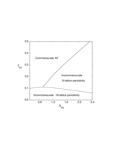
Figure 2: Phase diagram of stable antiferromagnetic state in the plane of $\Delta_{dp}=\epsilon_{p}-\epsilon_{d}$ and $t_{pp}$ obtained for $16\times 4$ lattice.

Figure 3: Energy of the coexistent state as a function of the SC order parameter for $x=0.125$ on $16\times 4$ lattice. We assume the incommensurate antiferromagnetic order (stripe). Parameters are $\epsilon_{p}=0$, $\epsilon_{d}=-2$ and $t_{pp}=0.4$.

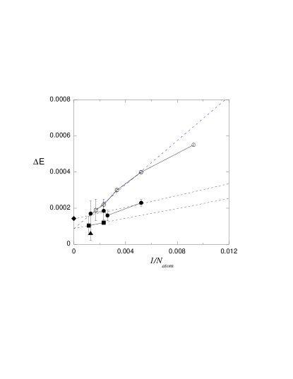
Figure 4: Energy gain due to the SC order parameter as a function of the system size $N_{atom}=3N_{s}$. Parameters are $\epsilon_{p}=0$, $\epsilon_{d}=-2$, $t_{pp}=0.4$, and $U_{d}=8$. The open circles are for the simple $d$-wave pairing at the hole density $x=0.2$. The solid symbols indicate the energy gain of the coexistent state: the solid circles are those at $x=0.125$, solid squares are those at $x=0.08333$ and the solid triangle is that at $x=0.0625$. The diamond shows the SC condensation energy obtained on the basis of specific heat measurements on the optimally doped YBa₂Cu₃O_6+x at $x=0.92$lor93 .

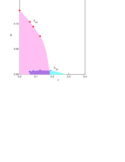
Figure 5: Phase diagram of the d-p model based on the Gutzwiller wave function.

The condensation energy $E_{cond}$ is defined as the difference $E_{cond}=E(\Delta\rightarrow 0)-E(\Delta)$ for the optimized energy. The energy of the antiferromagnetic state would be lowered further if we consider the incommensurate spin correlation in the wave function. The phase diagram in Fig. 2 presents the region of the stable AF phase in the plane of $t_{pp}$ and $\Delta_{dp}=\epsilon_{p}-\epsilon_{d}$. For large $\Delta_{dp}=\epsilon_{p}-\epsilon_{d}$, we have the region of the AF state with an eight-lattice periodicity in accordance with the results of neutron-scattering measurementstra96 ; wak00 . In the incommensurate antiferromagnetic region, we obtain a finite SC condensation energy, assuming a spatial oscillation, which is shown in Fig. 3. The variational parameters are $g=0.386$, $\tilde{\epsilon}_{d}=-1.578$, $\tilde{\epsilon}_{p}=0$, $\mu=-3.09$, $\Delta_{inc}=0.5$, and $\Delta=0.02$.

The main results of this study are shown in Fig. 4 where the size dependence of the SC condensation energy is shown for $x=0.2$, 0.125, 0.08333, and 0.0625. We set the parameters to be $\epsilon_{p}-\epsilon_{d}=2$ and $t_{pp}=0.4$ in $t_{dp}$ units, which is reasonable from the viewpoint of the density of states and in the region of eight-lattice periodicity at $x=1/8$. We have carried out the Monte Carlo calculations up to $16\times 16$ unit cells (768 atoms in total). In the overdoped region in the range of $0.18<x<0.28$, we have the uniform $d$-wave pairing state as the ground state. The periodicity of spatial variation judged from the condensation energy increases proportionally to $1/x$ as the doping rate $x$ decreases. In the figure, we have the 12-lattice periodicity at $x=0.08333$ and the 16-lattice periodicity at $x=0.0625$. For $x=0.2$, 0.125, and 0.08333, the results strongly suggest a finite condensation energy in the bulk limit. We believe that the size dependence of the SC condensation energy in the incommensurate region is rather weak because the main part of the superfluid density is in the hole-rich region of the striped structure. Thus we expect a finite condensation energy even at $x=0.08333$ and 0.0625. The SC condensation energy obtained on the basis of specific heat measurements agrees well with the result of variational Monte Carlo computationslor93 . In general, the Monte Carlo statistical errors are much larger than those for the single-band Hubbard model. A large number of Monte Carlo steps (more than 5.0$\times 10^{7}$) is required to obtain convergent expectation values for each set of parameters.

In Fig. 5 the order parameters $\Delta_{AF}$ and $\Delta_{SC}$ were evaluated using the formula $E_{cond}=(1/2)N(0)\Delta^{2}$ where $N(0)$ is the density of states. The SC condensation energy decreases as the doping rate $x$ is decreased because of the striped structure of the electronic state. Hence, $\Delta_{SC}$ also decreases. Here, we have set $N(0)\sim 5/t_{dp}$, since $N(0)$ is estimated to be $N(0)\sim 2$ to 3 $(eV)^{-1}$ for the optimally doped YBa₂Cu₃O_6+x using $N(0)(k_{B}T_{c})^{2}/2$and98 . The phase diagram is consistent with the recently reported phase diagram for layered cupratesmuk06 . Although the incommensurate order has never been observed in experiments, there is a possibility that observed commensurability of magnetic order may be brought about by the effect of nearby layers, that is, the cancellation of incommensurability between layers.

We examined the phase diagram of high-temperature superconductors with respect to the carrier density, on the basis of the d-p model. We carried out variational Monte Carlo calculations for the 2D d-p model to investigate the ground state for large $U_{d}$. In the lightly doped region we obtain the coexistent state of antiferromagnetism and superconductivity at the doping rate $x=0.125$, 0.0833 and 0.0625. As long as we employ the Gutzwiller ansatz, the ground state exhibits coexistence in the lightly doped region. In recent experimental works for layered cuprates, the possibility of the coexistent state of antiferromagnetism and superconductivity has been exploredmuk06 ; cri07 .

We express our sincere thanks to J. Kondo, S. Koikegami and S. Koike for helpful discussions. This work was supported by a Grant-in Aid for Scientific Research from the Ministry of Education, Culture, Sports, Science and Technology of Japan. Parts of the numerical calculations were performed at facilities of the Supercomputer Center of the Institute for Solid State Physics, University of Tokyo, and the Supercomputer Center of High Energy Accelerator Research Organization (KEK).

References

- (1) E. Dagotto: Rev. Mod. Phys. 66 (1994) 763.
- (2) The Physics of Superconductor Vol.II edited by K. H. Bennemann and J. B. Ketterson (Springer-Verlag, Berlin, 2003).
- (3) P. W. Anderson: The Theory of Superconductivity in the High-Tc Cuprates (Princeton University Press, Princeton, 1997).
- (4) T. Moriya and K. Ueda: Adv. Phys. 49 (2000) 555.
- (5) J. E. Hirsch, E. Y. Loh, D. J. Scalapino, and S. Tang: Phys. Rev. B39 (1989) 243.
- (6) R. T. Scalettar, D. J. Scalapino, R. L. Sugar, and S. R. White: Phys. Rev. B 44 (1991) 770.
- (7) T. Takimoto and T. Moriya: J. Phys. Soc. Jpn. 66 (1997) 2459.
- (8) M. Guerrero, J. E. Gubernatis, and S. Zhang: Phys. Rev. B 57 (1998) 11980.
- (9) A. Kobayashi, A. Tsuruta, T. Matsuura and Y. Kuroda: J. Phys. Soc. Jpn. 67 (1998) 2626.
- (10) S. Koikegami and K. Yamada: J. Phys. Soc. Jpn. 69 (2000) 768.
- (11) T. Yanagisawa, S. Koike and K. Yamaji: Phys. Rev. B 64 (2001) 184509.
- (12) S. Koikegami and T. Yanagisawa: J. Phys. Soc. Jpn. 70 (2001) 3499 (2001); J. Phys. Soc. Jpn. 71 (2002) 671.
- (13) T. Yanagisawa: New J. Physics 10 (2008) 023014.
- (14) C. Gros, R. Joynt, and T. M. Rice: Phys. Rev. B 36 (1987) 381.
- (15) H. Yokoyama and H. Shiba: J. Phys. Soc. Jpn. 56 (1987) 1490.
- (16) T. Nakanishi, K. Yamaji, and T. Yanagisawa: J. Phys. Soc. Jpn. 66 (1997) 294.
- (17) K. Yamaji, T. Yanagisawa, T. Nakanishi, and S. Koike: Physica C 304 (1998) 225.
- (18) J. Tranquada, J. Axe, D. Ichikawa, N. Nakamura, Y. Uchida, and B. Nachumi: Phys. Rev. B 54 (1996) 7489.
- (19) V. J. Emery: Phys. Rev. Lett. 58 (1987) 2794.
- (20) H. Eskes, G. A. Sawatzky, and L. F. Feiner: Physica C 160 (1989) 424.
- (21) M. S. Hybertson, E. B. Stechel, M. Schlüter, and D. R. Jennison: Phys. Rev. B 41 (1990) 11068.
- (22) A. K. McMahan, J. F. Annett, and R. M. Martin: Phys. Rev. B 42 (1990) 6268.
- (23) A. Himeda, T. Kato, and M. Ogata: Phys. Rev. Lett. 88 (2002) 117001.
- (24) M. Miyazaki, T. Yanagisawa, and K. Yamaji: J. Phys. Chem. Solids 63 (2002) 1403.
- (25) T. Giamarchi and C. Lhuillier: Phys. Rev. B 42 (1990) 10641.
- (26) T. Yanagisawa, S. Koike, and K. Yamaji, J. Phys.: Condens. Matter 14 (2002) 21.
- (27) T. Yanagisawa, S. Koike, S. Koikegami, and K. Yamaji: Phys. Rev. B 67 (2003) 132408.
- (28) M. Miyazaki, K. Yamaji, and T. Yanagisawa: J. Phys. Soc. Jpn. 73 (2004) 1643.
- (29) S. Wakimoto, R. J. Birgeneau, Y. Endoh, P. M. Gehring, K. Hirota, M. A. Kastner, S. H. Lee, Y. S. Lee, G. Shirane, S. Ueki, and K. Yamada: Phys. Rev. B 61 (2000) 3699.
- (30) J. W. Loram, K. A. Mirza, J. R. Cooper, and W. Y. Kiang: Phys. Rev. Lett. 71 (1993) 1740.
- (31) P. W. Anderson: Science 279 (1998) 1196.
- (32) H. Mukuda, M. Abe, Y. Araki, Y. Kitaoka, Y. Tokiwa, T. Watanabe, A.Iyo, H. Kito, Y. Tanaka: Phys. Rev. Lett. 96 (2006) 087001.
- (33) A. Crisan, Y. Tanaka, A. Iyo, D. D. Shivagan, P. M. Shirage, K. Tokiwa, T. Watanabe, L. Cosereanu, T. W. Button, and J. S. Abell: Phys. Rev. B 76 (2007) 212508.