Exact analytical results for quantum walks on star graph

Abstract

In this paper, we study coherent exciton transport of continuous-time quantum walks on star graph. Exact analytical results of the transition probabilities are obtained by means of the Gram-Schmidt orthonormalization of the eigenstates. Our results show that the coherent exciton transport displays perfect revivals and strong localization on the initial node. When the initial excitation starts at the central node, the transport on star graph is equivalent to the transport on a complete graph of the same size.

The problem of coherent and non-coherent transport modeled by random walks has attracted much attention in many distinct fields, ranging from polymer physics to biological physics, from solid state physics to quantum computation rn1 ; rn2 ; rn3 ; rn4 . Random walk is related to the diffusion models and a fundamental topic in discussions of Markov processes. Several properties of random walks, including dispersal distributions, first-passage times and encounter rates, have been extensively studied rn5 ; rn6 . As a natural extension to the quantum world of the ubiquitous classical random walks, quantum walks (QWs) have also been introduced and widely investigated in the literature rn7 .

An important application of quantum walks is that QWs can be used to design highly efficient quantum algorithms. For example, Grover s algorithm can be combined with quantum walks in a quantum algorithm for glued trees which provides even an exponential speed up over classical methods rn8 ; rn9 . Besides their important applications in quantum algorithms, quantum walks are also used to model the coherent exciton transport in solid state physics rn10 . It is shown that the dramatic nonclassical behavior of quantum walks can be attributed to quantum coherence, which does not exist in the classical random walks.

There are two main types of quantum walks: continuous-time and discrete-time quantum walks. The main difference between them is that discrete-time walks require a coin which is just any unitary matrix plus an extra Hilbert space on which the coin acts, while continuous-time walks do not need this extra Hilbert space rn11 . Apart from this difference, the two types of quantum walks are analogous to continuous-time and discrete-time random walks in the classical case rn11 . Discrete-time quantum walks evolve by the application of a unitary evolution operator at discrete-time intervals, and continuous-time quantum walks evolve under a time-independent Hamiltonian. Unlike the classical case, the discrete-time and continuous-time quantum walks cannot be simply related to each other by taking a limit as the time step goes to zero rn12 . Both the two types of quantum walks have been defined and studied on discrete structures in the market.

Here, we focus on continuous-time quantum walks (CTQWs). Most of previous studies related to CTQWs in the last decade concentrates on regular structures such as lattices, and most of the common wisdom concerning them relies on the results obtained in this particular geometry. Exact analytical results for CTQWs are also found for some particular regular structures, such as the cycle graph rn13 and Cayley tree rn14 . Exact analytical results are difficult to get due to the cumbersome analytical investigations of the eigenvalues and eigenstates of the Hamiltonian.

In this paper, we consider CTQWs on star graphs, and get exact analytical results for the first time. The star graph is one of the most regular structures in the graph theory and represents the local tree structure of the irregular and complex graphs. In mathematical language, a star graph of size $N$ consists of one central node and $N-1$ leaf nodes. All the leaf nodes connect to the central node, and there is no connection between the leaf nodes. Therefore, the central node has $N-1$ bonds and the leaf nodes have only one bond. As we will shown, for such simple topology, we are able to derive exact analytical results for the transition probabilities. These analytical results exactly agree with the numerical results obtained by diagonalizing the Hamiltonian $H$ using the software MATLAB.

The coherent exciton transport on a connected network is modeled by the continuous-time quantum walks (CTQWs), which is obtained by replacing the Hamiltonian of the system by the classical transfer matrix, i.e., $H=-T$ rn15 ; rn16 . The transfer matrix $T$ relates to the Laplace matrix by $T=-A$. The Laplace matrix $A$ has nondiagonal elements $A_{ij}$ equal to $-1$ if nodes $i$ and $j$ are connected and $0$ otherwise. The diagonal elements $A_{ii}$ equal to degree of node $i$, i.e., $A_{ii}=k_{i}$. The states $|j\rangle$ endowed with the node $j$ of the network form a complete, ortho-normalised basis set, which span the whole accessible Hilbert space. The time evolution of a state $|j\rangle$ starting at time $t_{0}$ is given by $|j,t\rangle=U(t,t_{0})|j\rangle$, where $U(t,t_{0})=exp[-iH(t-t_{0})]$ is the quantum mechanical time evolution operator. The transition amplitude $\alpha_{k,j}(t)$ from state $|j\rangle$ at time $0$ to state $|k\rangle$ at time $t$ reads $\alpha_{k,j}(t)=\langle k|U(t,0)|j\rangle$ and obeys Schrödinger s equation rn17 . Then the classical and quantum transition probabilities to go from the state $|j\rangle$ at time $0$ to the state $|k\rangle$ at time $t$ are given by $p_{k,j}(t)=\langle k|e^{-tA}|j\rangle$ and $\pi_{k,j}(t)=|\alpha_{k,j}(t)|^{2}=|\langle k|e^{-itH}|j\rangle|^{2}$ rn18 , respectively. Using $E_{n}$ and $|q_{n}\rangle$ to represent the $n$th eigenvalue and ortho-normalized eigenvector of $H$, the classical and quantum transition probabilities between two nodes can be written as rn17 ; rn18

$$p_{k,j}(t)=\sum_{n}e^{-tE_{n}}\langle k|q_{n}\rangle\langle q_{n}|j\rangle,$$ (1)

$$\pi_{k,j}(t)=|\alpha_{k,j}(t)|^{2}=|\sum_{n}e^{-itE_{n}}\langle k|q_{n}\rangle\langle q_{n}|j\rangle|^{2}.$$ (2)

For finite networks, the classical transition probabilities approach the equal-partition $1/N$. However, the quantum transport does not lead to equal-partition. $\pi_{k,j}(t)$ do not decay ad infinitum but at some time fluctuates about a constant value. This value is determined by the long time average of $\pi_{k,j}(t)$ rn17 ; rn18 ,

$$\begin{array}[]{ll}\chi_{k,j}&=\lim_{T\rightarrow\infty}\frac{1}{T}\int_{0}^{T}\pi_{k,j}(t)dt\\ &=\sum_{n,l}\langle k|q_{n}\rangle\langle q_{n}|j\rangle\langle j|q_{l}\rangle\langle q_{l}|k\rangle\\ &\ \ \ \ \times\lim_{T\rightarrow\infty}\frac{1}{T}\int_{0}^{T}e^{-it(E_{n}-E_{l})}dt\\ &=\sum_{n,l}\delta_{E_{n},E_{l}}\langle k|q_{n}\rangle\langle q_{n}|j\rangle\langle j|q_{l}\rangle\langle q_{l}|k\rangle.\end{array}$$ (3)

where $\delta_{E_{n},E_{l}}$ takes value 1 if $E_{n}$ equals to $E_{l}$ and 0 otherwise. In order to calculate $p_{k,j}(t)$, $\pi_{k,j}(t)$ and $\chi_{k,j}$, all the eigenvalues $E_{n}$ and eigenstates $|q_{n}\rangle$ are required. For the star graph, in the following, we will first analytically calculate the eigenvalues and eigenstates, then give exact analytical results for the transition probabilities according to the above Equations.

For a specific star graph of size $N$, we label the central node as node $1$ while the leaf nodes are numbered as $2,3,...,N$. Because of centrosymmetric structure of the star graph, there are only four types of transition probabilities, namely, $\pi_{1,1}(t)$, $\pi_{2,1}(t)\equiv\pi_{1,2}(t)$, $\pi_{2,2}(t)$ and $\pi_{3,2}(t)\equiv\pi_{2,3}(t)$. Transition probabilities between other nodes belong to these four types. Therefore, we only consider the four kinds of probabilities listed above. The Hamiltonian of the star graph can be written as,

$$H=(N-1)|1\rangle\langle 1|+\sum_{i=2}^{N}(|i\rangle\langle i|-|1\rangle\langle i|-|i\rangle\langle 1|).$$ (4)

The eigenvalues of the Hamiltonian have three discrete values: $E_{1}=E_{2}=...=E_{N-2}=1$, $E_{N-1}=0$ and $E_{N}=N$ add-ref . One set of eigenstates $\{|v_{i}\rangle\}$ ($i=1,2,...,N$) corresponding to the eigenvalues is : $|v_{i}\rangle=|i+2\rangle-|2\rangle$ ($i=1,2,...,N-2$), $|v_{N-1}\rangle=\sum_{i=1}^{N}|i\rangle$ and $|v_{N}\rangle=\sum_{i=1}^{N}|i\rangle-N|1\rangle$. However, this set of eigenstates are not orthogonal ($\langle v_{1}|v_{2}\rangle\neq 0$, etc), we use the Gram-Schmidt process rn19 to orthogonalize this set of eigenstates. The Gram-Schmidt algorithm is a method for orthogonalizing a set of vectors in an inner product space rn20 , the new orthogonal vectors $\{|v_{i}^{\prime}\rangle\}(i=1,2,...,N-2)$ are given by the following formula,

$$|v_{i}^{\prime}\rangle=|v_{i}\rangle-\sum_{j=1}^{i-1}\frac{\langle v_{i}|v_{j}^{\prime}\rangle}{\langle v_{j}^{\prime}|v_{j}^{\prime}\rangle}|v_{j}^{\prime}\rangle.$$ (5)

where $|v_{1}^{\prime}\rangle=|v_{1}\rangle$ is applied in the iterative process rn19 ; rn20 . According to the above equation, we obtain,

$$|v_{i}^{\prime}\rangle=\left\{\begin{array}[]{ll}|i+2\rangle-\frac{1}{i}\sum_{j=2}^{i+1}|j\rangle,&i=1,2,...,N-2\\ |v_{i}\rangle,&i=N-1,N.\end{array}\right.$$ (6)

The above new eigenstates $\{v_{i}^{\prime}\rangle\}$ is not normalized (i.e., $\langle v_{i}^{\prime}|v_{i}^{\prime}\rangle\neq 1$, etc). After some algebraic calculations, we get the orthonormal basis $\{|q_{i}\rangle\}$ as follows,

$$|q_{i}\rangle=\left\{\begin{array}[]{lll}\sqrt{\frac{i}{i+1}}|i+2\rangle-\sqrt{\frac{1}{i(i+1)}}\sum_{j=2}^{i+1}|j\rangle,&i=1,2,...,N-2\\ \sqrt{1/N}\sum_{j=1}^{N}|j\rangle,&i=N-1\\ \frac{1}{\sqrt{N(N-1)}}\sum_{i=1}^{N}|i\rangle-\sqrt{\frac{N}{N-1}}|1\rangle,&i=N.\end{array}\right.$$ (7)

One can easily prove $\{|q_{i}\rangle\}$ is also a set of eigenstates of the Hamiltonian (i.e., $H|q_{i}\rangle=E_{i}|q_{i}\rangle,\forall\ i$). $\{|q_{i}\rangle\}$ forms an orthonormal and complete basis, satisfying $\langle q_{i}|q_{j}\rangle=\delta_{ij}$ and $\sum_{j}|q_{j}\rangle\langle q_{j}|=1$. Therefore, we can use this set of eigenstates $\{|q_{i}\rangle\}$ to calculate the transition probabilities in Eqs. (1), (2) and (3).

Substituting the orthonormal basis of Eq. (7) into Eqs (2), we get $\pi_{1,1}(t)$ and $\pi_{2,1}(t)$ as follows,

$$\pi_{1,1}(t)=\frac{N^{2}-2N+2}{N^{2}}+\frac{2(N-1)}{N^{2}}\cos Nt.$$ (8)

$$\pi_{2,1}(t)=\frac{2}{N^{2}}-\frac{2}{N^{2}}\cos Nt.$$ (9)

For $\pi_{2,2}(t)$ and $\pi_{3,2}(t)$, the calculation is analogous, but the expressions are cumbersome:

$$\begin{array}[]{ll}\pi_{2,2}(t)&=\frac{1}{N^{2}(N-1)^{2}}[(N^{4}-4N^{3}+5N^{2}-2N+2)\\ &+(2N^{3}-6N^{2}+4N)\cos t\\ &+(2N^{2}-4N)\cos(N-1)t\\ &+(2N-2)\cos Nt].\end{array}$$ (10)

$$\begin{array}[]{ll}\pi_{3,2}(t)&=\frac{2}{N^{2}(N-1)^{2}}[(N^{2}-N+1)\\ &+(N-N^{2})\cos t-N\cos(N-1)t\\ &+(N-1)\cos Nt].\end{array}$$ (11)

Other transition probabilities can also calculated, but they have the same expressions as Eqs (8)$\sim$(11). For instance, $\pi_{4,2}(t)$ has the same analytical form as $\pi_{3,2}$, which is consistent with our intuition. Analogously, we can get the long time averages of the transition probabilities:

$$\begin{array}[]{ll}\chi_{1,1}=(N^{2}-2N+2)/N^{2}\\ \chi_{2,1}=2/N^{2}\\ \chi_{2,2}=(N^{4}-4N^{3}+5N^{2}-2N+2)/N^{2}/(N-1)^{2}\\ \chi_{3,2}=2(N^{2}-N+1)/N^{2}/(N-1)^{2}.\end{array}$$ (12)

The transition probabilities depend on the size of the graph. In the thermodynamic limit of infinite network $N\rightarrow\infty$, the transport displays high localizations on the initial position, i.e., $\chi_{i,j}\approx\delta_{i,j}$. On the contrary, for the classical transport modeled by continuous-time random walks, the transition probabilities do not show any oscillation and approach to the equal-partition $1/N$ at long times add-ref . According to Eq. (1), the four type transition probabilities can be written as,

$$\begin{array}[]{ll}p_{1,1}(t)=1/N+e^{-Nt}(N-1)/N\\ p_{2,1}(t)=1/N-e^{-Nt}/N\\ p_{2,2}(t)=1/N+(N-2)/(N-1)e^{-t}+e^{-Nt}/N/(N-1)\\ p_{3,2}(t)=1/N-e^{-t}/(N-1)+e^{-Nt}/N/(N-1).\end{array}$$ (13)

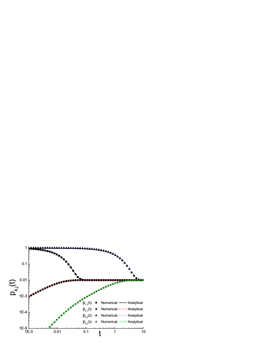
Figure 1: (Color online)Classical transition probabilities $p_{k,j}(t)$ versus $t$. The marked points are numerical results and the curves are analytical predictions in Eq. (13).

In order to test the analytical predictions, we compare the classical $p_{k,j}(t)$ predicted by Eq. (13) with the numerical results obtained by numerically diagonalizing the Hamiltonian. The results for a star graph of $N=100$ are shown in Fig. 1. As we can see, the numerical results exactly agree with the analytical prediction in Eq. (13). The transport reaches the equal-partitioned distribution $1/N$ at long times. However, when the excitation starts at the central node, the transport reaches the equal-partition more quickly than the transport which starts at the leaf nodes (Compare the curves in Fig. 1).

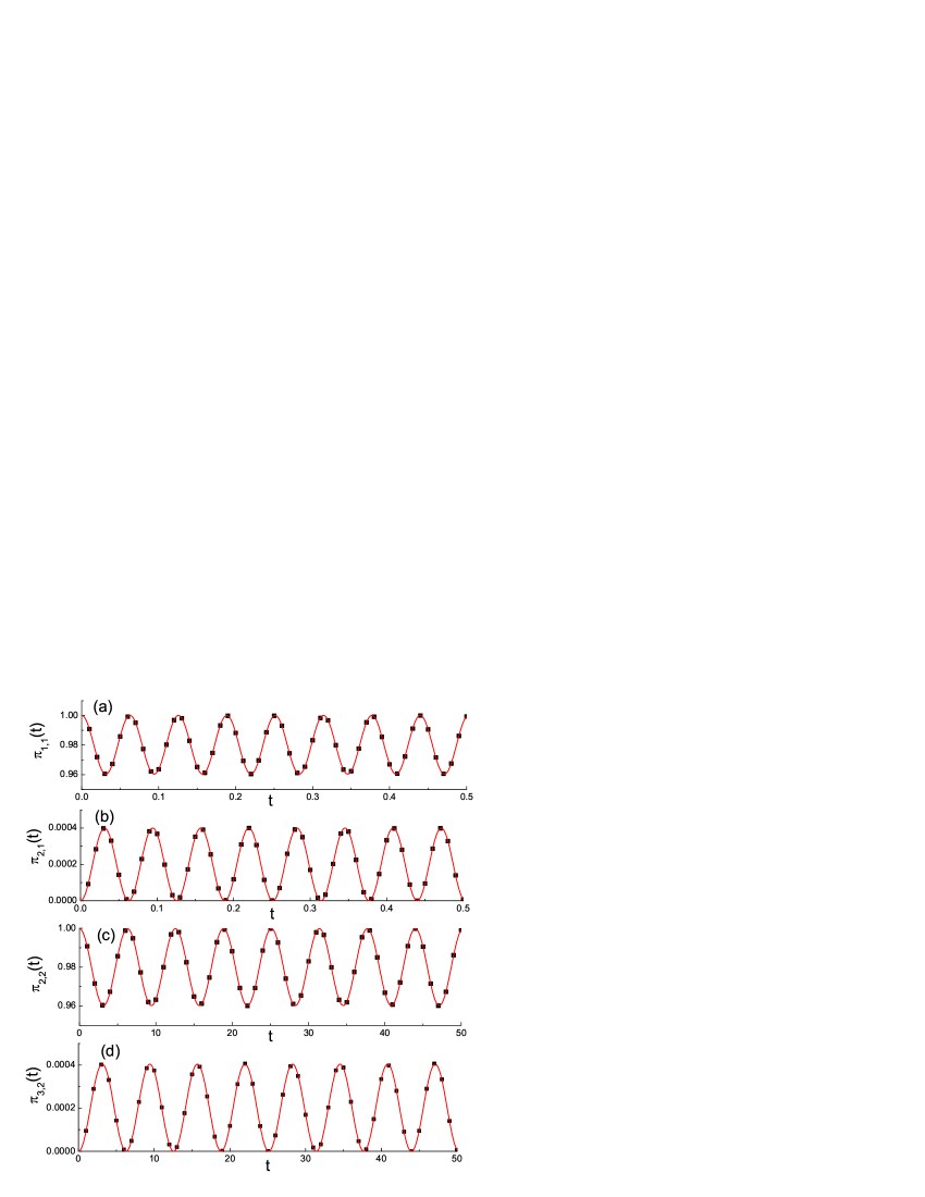
Figure 2: (Color online)Quantum transition probabilities $\pi_{1,1}(t)$ (a), $\pi_{2,1}(t)$ (b), $\pi_{2,2}(t)$ (c) and $\pi_{3,2}(t)$ (d). The points denoted by black squares are numerical results and the curves are theoretical predictions in Eqs. (8)-(11).

For the quantum transport, we compare the transition probabilities in Fig. 2. The numerical results (marked as black squares) exactly agree with the theoretical results in Eqs. (8)-(11). We note that all the transition probabilities show periodic recurrences. Comparing $\pi_{1,1}(t)$ and $\pi_{2,2}(t)$ (See Fig. 2 (a) and (c)), we find that there are high probabilities to find the exciton at the initial node. This suggests that the coherent transport shows high localizations on the initial nodes add-ref . The oscillation amplitudes of the return probabilities $\pi_{1,1}(t)$ and $\pi_{2,2}(t)$ are comparable but the oscillation periods are quite different. The oscillating period of $\pi_{2,2}(t)$ is $100$ (N) times of that of $\pi_{1,1}(t)$. This could be interpreted by the analytical expressions in Eqs. (8) and (10). Similar behavior also holds for $\pi_{2,1}(t)$ and $\pi_{3,2}(t)$ (See Fig. 2 (b) and (d)), but the oscillation amplitude is smaller than the return probabilities. This also can be understood from the analytical results in Eqs. (9) and (11), where the transition probability is mainly determined by the high order term of $N$. The small value of oscillating period of $\pi_{2,1}(t)$ and $\pi_{1,1}(t)$ suggests that there are frequent revivals when the exciton starts at the central node, compared to the transport starting at the leaf nodes.

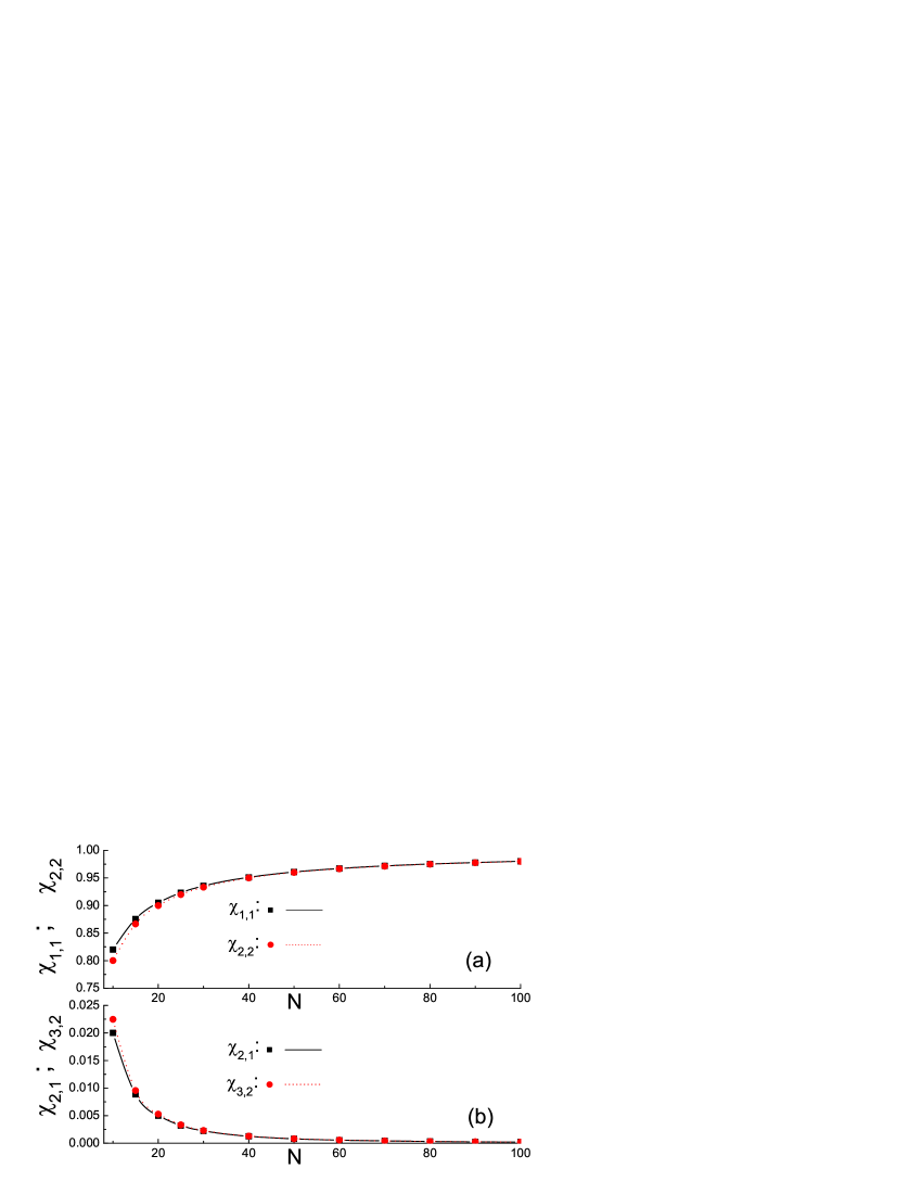
Figure 3: (Color online)Long-time limiting probabilities $\chi_{1,1}$, $\chi_{2,2}$ (a) and $\chi_{2,1}$, $\chi_{3,2}$ (b) as a function of the network size $N$. The points marked as symbols are numerical results and the curves are analytical results predicted by Eq. (12).

The quantum limiting probabilities in Eq. (12) are only a function of graph size $N$. Fig. 3 shows the quantum limiting probabilities for numerical results and theoretical predictions. Both the results agree with each other. We find that the return probabilities $\chi_{1,1}$ and $\chi_{2,2}$ are an incremental function of $N$ and approach to $1$ in the limit $N\to\infty$. By contraries, $\chi_{2,1}$ and $\chi_{3,2}$ decrease with $N$ and close to $2/N^{2}$ in the limit $N\to\infty$. We note that $\chi_{1,1}$ differs from $\chi_{2,2}$ for small values of $N$. Such deviation diminishes as $N$ increases. This suggests that the strength of localizations is almost the same for central-node and leaf-node excitations. The only difference is that the frequency of revivals (oscillation period) for central node excitation is much higher than that for leaf node excitation.

To address the similarity and difference between the star graph and complete graph, we proceed to consider the transport on a complete graph of size $N$. The complete graph is fully connected, thus the Hamiltonian is given by $H=(N-1)\sum_{i}|i\rangle\langle i|-\sum_{i\neq j}|i\rangle\langle j|$. The eigenvalues are two different values: $E_{1}=E_{2}=...=E_{N-1}=N$ and $E_{N}=0$. One set of un-orthogonal states $\{|v_{i}\rangle\}$ corresponding to the eigenvalues can be written as: $|v_{i}\rangle=|i+1\rangle-|1\rangle$ ($i=1,2,...,N-1$) and $|v_{N}\rangle=\sum_{j=1}^{N}|j\rangle$. Using the Gram-Schmidt orthonormalization (See Eq. (5)), the orthonormal basis for a complete graph is,

$$|q_{i}\rangle=\left\{\begin{array}[]{lll}\sqrt{\frac{i}{i+1}}|i+1\rangle-\sqrt{\frac{1}{i(i+1)}}\sum_{j=1}^{i}|j\rangle,&i=1,2,...,N-1\\ \sqrt{1/N}\sum_{j=1}^{N}|j\rangle,&i=N.\\ \end{array}\right.$$ (14)

Substituting the above Equation into Eq. (2), we get the quantum transition probabilities for complete graph,

$$\pi_{i,j}(t)=\left\{\begin{array}[]{lll}\frac{N^{2}-2N+2}{N^{2}}+\frac{2(N-1)}{N^{2}}\cos Nt,&i=j\\ \frac{2}{N^{2}}-\frac{2}{N^{2}}\cos Nt.&i\neq j.\\ \end{array}\right.$$ (15)

We note that Eq. (15) is exactly the same form as Eqs. (8) and (9). This indicates that the transport starting at central node on star graph is equivalent to the transport on a complete graph of the same size.

In summary, we have studied coherent exciton transport of continuous-time quantum walks on star graph. Exact analytical results of the transition probabilities are obtained in terms of the Gram-Schmidt orthonormalization. We find that the coherent transport shows perfect recurrences and there are high frequency of revivals for central node excitation. Study of long time averages suggests that the quantum transport displays strong localizations on the initial node. When the initial excitation starts at the central node, the transport on star graph is equivalent to the transport on a complete graph of the same size.

This work is supported by National Natural Science Foundation of China under projects 10575042, 10775058 and MOE of China under contract number IRT0624 (CCNU).

References

- (1) N. Guillotin-Plantard and R. Schott, Dynamic Random Walks: Theory and Application (Elsevier, Amsterdam, 2006).
- (2) W. Woess, Random Walks on Infinite Graphs and Groups (Cambridge: Cambridge University Press, 2000).
- (3) D. Supriyo, Quantum Transport: Atom to Transistor (Cambridge University Press, London, 2005).
- (4) P. A. Mello and N. Kumar, Quantum Transport in Mesoscopic Systems: Complexity and Statistical Fluctuations (Oxford University Press, USA, 2004).
- (5) R. Metzler und J. Klafter, Phys. Rep. 339, 1 (2000).
- (6) R. Burioni and D. Cassi, J. Phys. A 38, R45 (2005).
- (7) E. Farhi and S. Gutmann, Phys. Rev. A 58, 915 (1998).
- (8) L. K. Grover, A Fast Quantum Mechanical Algorithm for Database Search, Proceedings of the Twenty-Eighth Annual ACM Symposium on Theory of Computing pp. 212 C219( ACM, New York, 1996).
- (9) Y. Yin, D. E. Katsanos, and S. N. Evangelou, Phys. Rev. A 77, 022302 (2008).
- (10) C. Kittel, Introduction to solid state physics (Wiley, New York, 1986).
- (11) H. Krovi and T. A. Brun, Phys. Rev. A 75, 062332 (2007).
- (12) F. W. Strauch, Phys. Rev. A 74, 030301R (2006).
- (13) D. Solenov and L. Fedichkin, Phys. Rev. A 73, 012313(2003).
- (14) O. Mülken and A. Blumen, Phys. Rev. E 71, 016101 (2005).
- (15) O. Mülken and A. Blumen, Phys. Rev. E 71, 036128 (2005).
- (16) X. P. Xu, W. Li and F. Liu, arxiv.quan-ph/0810.0824 (2008).
- (17) A. Volta, O. Mülken and A. Blumen, J. Phys. A 39, 14997 (2006).
- (18) X. P. Xu, Phys. Rev. E 77, 061127 (2008).
- (19) O. Mülken and A. Blumen, Phys. Rev. E 73, 066117 (2006).
- (20) http://www.math.hmc.edu/calculus/tutorials/gramschmidt/
- (21) G. Arfken, Mathematical Methods for Physicists, pp. 516-520 (3rd ed. Orlando, Academic Press, 1985).