We propose a method for analyzing Berry phase for a multi-qubit system of superconducting charge qubits interacting with a microwave field. By suitably choosing the system parameters and precisely controlling the dynamics, novel connection found between the Berry phase and entanglement creations.

PACS numbers: 74.70.-b, 03.65.Ta, 03.65.Yz, 03.67.-a, 42.50.-p

1 Introduction

Berry’s phase [1] can be thought of as an adiabatic quantum holonomy restricted to a one-dimensional energy eigenspace [2]. The Berry phase has very interesting applications, such as the implementation of quantum computation by geometric means [3, 4, 5]. Recently, it has been recognized that large-scale quantum computers are hard to construct because quantum systems easily lose their coherence through interaction with the environment [2]. Researchers have tried to avoid this problem by using geometric phase shifts in the design of quantum gates to perform information processing. The robustness of Berry’s geometric phase for spin-1/2 particles in a cyclically varying magnetic field has been tested experimentally [6]. Interesting Berry phase results of a composite system have also been presented in [7] and a new formalism of the geometric phase for mixed states in the experimental context of quantum interferometry has been discussed in Ref. [8]. In another set of experiments, Du et al. [9] performed an NMR experiment to measure the geometric phase for mixed quantum states, and Leek et al. [10] analyzed experimentally the Berry phase for a superconducting qubit affected by parameter fluctuations.

Another important problem associated with quantum computation and information is the problem of engineering entanglement in multi-particle systems. This has attracted a great deal of recent interest [11, 12, 13, 14]. Here questions of how the couplings among the subsystems changes the Berry phase of the composite system become of great importance. In this regard, the relation between entanglement and the Berry phase has been discussed in solid state systems [15] and in icosahedral Jahn-Teller systems [16]. Most of the earlier works on the geometrical phase focus on pure quantum states [17, 18, 19, 20, 21]. These types of systems, however, are very unrealistic and almost never occur in practice. In some applications, however, in particular geometric fault tolerant quantum computation [3], mixed state cases are important. From a mathematical point of view, Uhlmann was the first to address the issue of mixed state holonomy [22, 23]. The difficulty with mixed states is their reduced coherence, which makes any notion of a phase more difficult to define and measure. Another challenge for the future is to extend this work to more general forms of mixed state multi-qubit systems.

The aim of the present work is to develop a general treatment of the multi-qubit problem and develop realizable procedures to various base spaces. This is dome treating the non-degenerate time evolution operator and satisfying parallel transport evolution condition and by defining the Berry phase in a new, rather simple, way. In particular, one of the most important problems under consideration is how to define the Berry phase of multi-qubit system and easy-monitored entangled state with existing experimental techniques [24]. We will show that setting up an arrangement in which an entanglement can be measured via the Berry phase for superconducting qubits is an interesting task both from the experimental and theoretical viewpoints.

2 Mixed state Berry phase

The Berry phase has been extensively studied [7, 25, 26, 27] and generalized in various ways. For example, based on the fact that any mixed state can be represented as a pure one if one allows ancillas and optimizes over many purification, the mixed state geometric phase has been defined [8], for open systems [28], and with a quantized field driving [29].

To study the geometric properties of a quantum system [30], we evaluate the Berry phase of the system by introducing a phase shift operator

$$R(t)=\exp[-i\phi(t)\psi^{{\dagger}}\psi],$$ (1)

where $\phi(t)$ is changed from $0$ to $2\pi$ adiabatically. We denote by $\psi^{\dagger}(\psi)$ the creation (annihilation) operator of the cavity mode. Then the time independent eigenequation of the system $H|\chi_{j}\rangle=\Im_{j}|\chi_{j}\rangle,$ is changed into $H^{\prime}|\chi_{j}^{\prime}\rangle=\Im_{j}^{\prime}|\chi_{j}^{\prime}\rangle$, with

$$H^{\prime}=R(t)HR^{{\dagger}}(t)-iR(t)\frac{dR^{{\dagger}}(t)}{dt},$$ (2)

and $|\chi_{j}^{\prime}\rangle=R(t)|\chi_{j}\rangle$. Hence, the Berry phase generated after the system undergoing an adiabatic and cyclic evolution may be calculated as follows

$$\gamma_{j}(\tau)=i\int\limits_{0}^{\tau}\langle\chi_{j}|R^{{\dagger}}(t)\frac{dR(t)}{dt}|\chi_{j}\rangle dt.$$ (3)

Whenever a pure quantum state undergoes a parallel transport along a closed path, it gathers information on the geometric structure of the Hilbert space in which it lies. On the other hand, a state of subsystem is no longer a pure one and to study the Berry phase of the subsystem (a non-degenerate density matrix), we have to adopt the definition of geometric phase for a mixed state [8]. Our goal in the following is to establish a connection between the Berry phase acquired by a multi-qubit system and the Berry phases of the subsystem.

The geometric phase corresponding to the non-unitary evolution can be defined according to the geometric phase of the whole system that evolves unitarily. For example, let us consider the following mixed state

$$\rho(t)=\sum\limits_{k=1}^{L}\xi_{k}U(t)\rho_{k}(0)U^{{\dagger}}(t),$$ (4)

where $\rho_{k}(0)$ is an orthonormal set of pure states and $\xi_{k}$ is the probability, where, $\rho(0)=\sum_{k=1}^{L}\xi_{k}\rho_{k}(0)$ and $L$ is the total number of the involved pure states. For non-degenerate $\xi_{k}$ the time evolution operator is given by $U(t)=U_{0}(t)\sum_{k}e^{-i\alpha_{k}}$ $\rho_{k}(0),$ where $\alpha_{k}$ are arbitrary real parameters and $U_{0}(t)$ is one of the equivalent operators to $U(t)$. When a mixed state given by the density matrix $\rho(t)$ evolves under a unitary operator $U(t),$ the parallel transport evolution condition is

$$Tr[\rho_{k}(t)\overset{.}{U}(t)U^{{\dagger}}(t)]=0,\ (k=1,2,...,L).$$ (5)

Based on geometric phase definition for a mixed state [8] and using Eqs. (4) and (5), for an adiabatic cyclic evolution, a new definition of the Berry phase for a mixed states can be written as

$$\gamma_{B}(\tau) = \arg\left\{\sum\limits_{k=1}^{L}\text{Tr}\left[\xi_{k}\rho_{k}(0)U_{1}(\tau)\right.\right.$$ (6)

$$\left.\left.\times\exp\left(-\int\limits_{0}^{\tau}\text{Tr}[\rho_{k}(0)U_{0}^{{\dagger}}(t)\overset{.}{U}_{0}(t)]dt\right)\right]\right\}.$$

The Berry phase Eq. (6) for a mixed state is just an average of the individual Berry phases. The Berry phase factor for a mixed state defined by Eq. (6) is a weighted sum of the one-particle Berry phase factors. In the pure state case Eq. (6) is consistent with the result of Eq. (3).

2.1 Multi-qubit system

Over the last decade, superconducting qubits have gained substantial interest as an attractive option for quantum information processing [31, 32, 33] and Josephson qubits are among the most promising devices to implement solid state quantum computation [34, 35]. A novel method for the controlled coupling of two Josephson charge qubits by means of a variable electrostatic transformer has been proposed in Ref. [36] and the behavior of charge oscillations in superconducting Cooper pair boxes weakly interacting with an environment has been discussed [38]. Also, the quantum dynamics of a Cooper-pair box with a superconducting loop in the presence of a nonclassical microwave field have been investigated in Ref. [39].

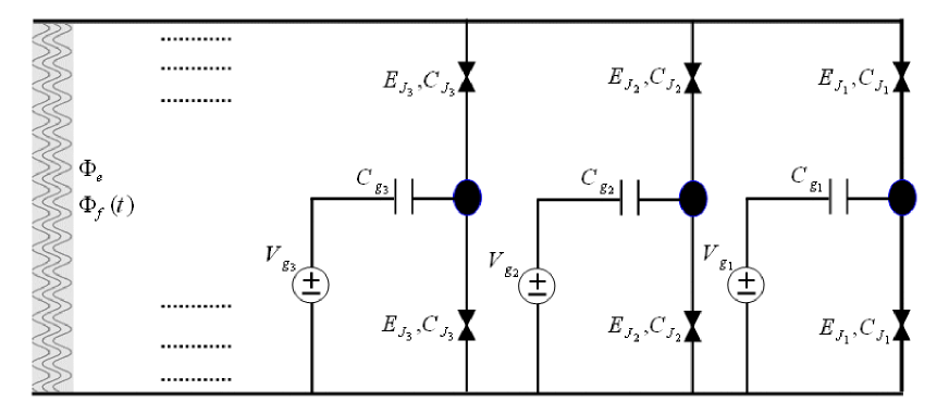
Figure 1: Schematic picture of the multi-Cooper-pair-box system. The filled circle denotes a superconducting island or the Cooper-pair box. It is biased by a voltage $V_{g_{i}}$ through the gate capacitance $C_{g_{i}}$ and coupled to the bulk superconductors by two identical small Josephson junctions. The two Josephson junctions have capacitance $C_{J_{i}}$ and Josephson energy $E_{Ji}$. The total flux is the summation of the static magnetic flux $\Phi_{e}$, and microwave-field-induced flux $\Phi_{f}(t)$ applied via the SQUID loop.

As an explicit example, we consider a suitable multi-qubit system and envisage a process in which the qubits interact with the microwave cavity such that there is no overlap of their interactions. Let us start with a short description of a superconducting box formed from a low-capacitance Josephson junction of capacitance $C_{J_{i}}$ and Josephson energy $E_{J_{i}}.$ The Josephson junction is biased by a voltage source $V_{g_{i}}$ through a gate capacitance $C_{g_{i}}$ which is externally controlled and used to induce offset charges on the island. The schematic picture of this multi-qubit structure is shown in figure 1. The total Hamiltonian of the single-Cooper pair box system can be written as [40]

$$\hat{H} = \hbar\omega_{k}(\widehat{\psi}^{\dagger}\widehat{\psi}+\frac{1}{2})$$ (7)

$$+\frac{(Q-C_{g_{i}}V_{g_{i}})^{2}e}{C_{g_{i}}+2C_{J_{i}}}-2E_{J0}\cos\phi\cos\left(\pi\frac{\Phi}{\Phi_{0}}\right),$$

where $\widehat{\psi}^{\dagger}(\widehat{\psi})$ is the creation (annihilation) operator of the cavity mode. In this structure, the superconducting island with Cooper-pair charge $Q=2Ne$ is coupled to a segment of a superconducting ring via two Josephson junctions, where $e$ is the electron charge and $N$  is the number of Cooper-pairs. We denote by $\phi=0.5(\phi_{1}+\phi_{2})$ the phase difference across the junction. The gauge-invariant phase drops $\phi_{1}$ and $\phi_{2}$ across the junctions are related to the total flux $\Phi$ through the SQID loop by the constraint $\phi_{2}-\phi_{1}=2\pi\Phi/\Phi_{0},$ where $\Phi_{0}=h/2e$ is the quantum flux. We assume that the structure of the Cooper pair box is characterized by two energy scales, i.e., the charging energy $E_{c}$ and the coupling energy $E_{J_{0}}$ of the Josephson junction, and we consider that the charging energy with scale $Ec=e^{2}/2(C_{g}+C_{J})$ is chosen to dominate over the Josephson coupling energy $E_{J}$ and weak quantized radiation field, so that only the two low-energy charge states $N=0$ ($\left|0\right\rangle$) and $N=1$($\left|1\right\rangle$) are relevant [41] while all other charge states, having a much higher energy, can be ignored. When a nonclassical microwave field is applied, the total flux is a quantum variable $\Phi=\Phi_{e}+\Phi_{f}(t),$ where $\Phi_{f}$ is the microwave-field-induced flux. If we consider a planar cavity containing the superconducting-quantum-interference-device loop of the charge qubit perpendicular to the cavity mirrors, the vector potential of the nonclassical microwave field can be written as $A(r)=|u_{k}(r)|(\widehat{\psi}^{\dagger}+\widehat{\psi})\widehat{A},$ where a single-qubit structure is embedded in the microwave cavity with only a single photon mode $\lambda.$ Thus, the flux $\Phi_{f}$ can be written as $\Phi_{f}=|\Phi_{k}|(\widehat{\psi}^{\dagger}+\widehat{\psi}),$ where $\Phi_{k}=\oint u_{k}.dl.$ We shift the gate voltage $V_{g}$ (and/or vary $\Phi_{e}$) to bring the single-qubit system into resonance with $k$ photons: $E\approx k\hbar\omega_{k}$, $k=1,2,3,....$ Note that the charge states are not the eigenstates of the Hamiltonian (8), so that the Hamiltonian can be diagonalized yielding the following two charge states $|e\rangle=\cos\eta\left|1\right\rangle-\sin\eta\left|0\right\rangle$ and $|g\rangle=\sin\eta\left|1\right\rangle+\cos\eta\left|0\right\rangle$ with $\eta=\frac{1}{2}\tan^{-1}(E_{J}/2\varepsilon),$ where $\varepsilon=2E_{ci}(C_{gi}V_{gi}e^{-1}-(2n+1)).$ Employing these eigenstates to represent the qubits, expanding the functions $\cos(\pi\Phi/\Phi_{0})$ and using the rotating wave approximation, one can derive the total Hamiltonian of the system as [31, 41]

$$\hat{H} = \hbar\omega_{k}(\widehat{n}+\frac{1}{2})$$ (8)

$$+\sum\limits_{j=1}^{m}\left\{\frac{1}{2}E-E_{J0}^{(j)}\sin\left(2\eta\right)\cos\left(\frac{\pi\Phi_{e}}{\Phi_{0}}\right)f(\widehat{n})\right\}\sigma_{z}^{(j)}$$

$$+\sum\limits_{j=1}^{m}\left\{E_{J0}^{(j)}\cos\left(2\eta\right)\psi^{k}g_{{}_{(k)}}(\widehat{n})\sigma_{+}^{(j)}+H.c.\right\}.$$

Here we denote by $\sigma_{\pm}^{(j)}$ and $\sigma_{z}^{(j)}$ the Pauli matrices in the pseudo-spin basis of the $j^{th}$ qubit and $g_{k}(\widehat{n}),$ ($\widehat{n}=\widehat{\psi}^{\dagger}\widehat{\psi}$) represents the $k-$photon-mediated coupling between the charge qubit and the microwave field.

The influence of entanglement on the noncyclic two-particle geometric phase has been studied for an entangled spin pair in Refs. [8, 42, 43]. It was shown that prior entanglement shared between the two spins can change the Berry phase in such an entangled pair. Also, an experimental technique for preparing arbitrarily entangled polarization states has been developed [44]. The treatment here extends these investigations to explore, in a controlled setting, the fundamental features of the relation between Berry-phase and entanglement in multi-qubit system. In particular, we consider a process in which multiple superconducting charge qubits are placed in parallel and in addition to a static magnetic flux, a microwave field is applied through the SQUID loop. Also, each qubit interacts with the microwave field such that there is no overlap of their interaction with the field or with each other [45, 46]. In a similar model [47], multiple charge qubits are placed in parallel and coupled via a common inductance.

2.2 Numerical results

Figure 2: Berry phase $\gamma_{B}(t)$ and entropy corresponding to the first instantaneous eigenstate versus the dimensionless detuning parameter $\Delta/\lambda$ $(\lambda=\sqrt{e^{2}\omega/(\hbar C_{F}}),$ for different number of n. Here the curves are for $n=0$ (solid curve) and $n=10$ (dotted curve). The plot was normalized and presented in units of  $\pi$ for the Berry phase.

In order to understand a number of different cases, we show, in what follows, plots of the Berry phase for different values of the involved parameters. As might be expected, the behavior of the present system changes depending on the number of Cooper pair boxes (qubits) involved, the variation of the system parameters, i.e., the Josephson energy $E_{J_{i}},$ gate capacitance $C_{g_{i}}$ and initial state of the field. The Berry’s phase defined in equation (6) is calculated using quantum states evolving in time under the action of Hamiltonian $\hat{H}$.  If the evolution of only one qubit is considered, it is straightforward to write down the formal solution of the problem as $\hat{H}|s,g\rangle=\Omega_{0}|s,g\rangle,\quad 0\leq s<k$  and $\hat{H}|\Phi_{\pm}^{(n)}\rangle=\Omega_{\pm}^{(n)}|\Phi_{\pm}^{(n)}\rangle,$ where $\Omega_{0}$ and $\Omega_{\pm}^{(n)}$ are the eigenvalues. The entangled states $|s,g\rangle$ and $|\Phi_{\pm}^{(n)}\rangle$ are orthonormal and complete. Here $\pm$, labels the entangled states which in their bare condition are the ground $|g\rangle$ and the excited $|e\rangle$ states, and $n$, the states of the boson field. The unitary operator $\hat{U}(t)$ can be written as

$$\hat{U}(t) = \sum\limits_{n=0}^{\infty}\sum\limits_{l=+,-}\left\{\exp(-it\Omega_{l}^{(n)})|\Psi_{l}^{(n)}\rangle\langle\Psi_{l}^{(n)}|\right\}$$ (9)

$$+\sum\limits_{s=0}^{k-1}\exp(-it\Omega_{0})|s,g\rangle\langle g,s|.$$

In Fig. (2), we use Eq. (9) and assume that the qubits initially prepared in the excited level interact with the cavity under consideration are in the pure number state (Fock state), i.e. $\hat{\rho}_{f}\left(0\right)=|n\rangle\langle n|$. In this figure we show the measured Berry phase $\gamma_{B}(\tau)$ and its dependence on the scaled detuning $\Delta/\lambda,$ ($\lambda=\sqrt{e^{2}\omega/(\hbar C_{F}})$, for different value of $n$. The calculations are all carried out with the single photon process and $\Phi_{e}=\Phi_{0}/2$ for all Josephson charge qubits. Here two parameters are varied; the number $n$ and the dimensionless detuning parameter $\Delta/\lambda$. The measured phase is in all cases seen to be exponentially decay with the development of the detuning. Detuning is expected to have the same influence on Berry’s phase and entanglement. This characteristic robustness of Berry phases may be exploitable in the realization of logic gates for quantum computation. To compare the Berry phase with entanglement, we use the von Neumann entropy, $S(t)=Tr[\hat{\rho}\left(t\right)\ln\hat{\rho}\left(t\right)]$. The quantum dynamics described by the Hamiltonian (8) leads to an entanglement between the field and the qubits. We can express the entropy $S(t)$ in terms of the eigenvalue $\Upsilon_{i}(t)$ of the reduced density operator [24], as $S(t)=-\sum_{i}\Upsilon_{i}(t)\ln\Upsilon_{i}(t).$ For a single qubit, disentangled pure joint state leads to $S(t)$ is zero, and for maximally entangled states the entropy gives $\ln 2$.  In our consideration to the behavior of the entropy as a function of the detuning parameter $\Delta/\lambda$. When we take $\Delta/\lambda=0$, we get almost maximum value for the entropy. As the detuning parameter is increased, the entropy as well as the Berry phase are decreased. Further increasing of the detuning leads to vanishing of both $\gamma_{B}(\tau)$ and $S(t),$ which means a completely pure state is reached (see figure 2).

In the two qubits case, the eigenstates can be written as

$$|\psi_{n}^{(j)}\rangle=\sum_{i=1}^{4}a_{i}^{(j)}(n)|\Phi_{i}\rangle,$$ (10)

where ($|\Phi_{i}\rangle=|e,e,n\rangle,|e,g,n+k\rangle,|g,e,n+k\rangle,|g,g,n+2k\rangle),$ which have an additional phase comes from a geometrical feature [48], i.e., the Berry phase is given by

$$\gamma_{n}=2\pi(|a_{1}(n)|^{2}-|a_{4}(n)|^{2}).$$ (11)

For the density matrix $\hat{\rho}(t)=|\psi_{n}^{(j)}\rangle\langle\psi_{n}^{(j)}|,$ which represents the state of a bipartite system, concurrence is defined as

$$C(\hat{\rho})=\max[0,\lambda_{1}-\lambda_{2}-\lambda_{3}-\lambda_{4}],$$ (12)

where the $\lambda_{i}$ are the non-negative eigenvalues, in decreasing order ($\lambda_{1}\geq\lambda_{2}\geq\lambda_{3}\geq\lambda_{4}$), of the Hermitian matrix ${\Upsilon}\equiv\sqrt{\sqrt{\hat{\rho}}\widetilde{\rho}\sqrt{\hat{\rho}}}$ and $\widetilde{\rho}=\left({\sigma}_{y}\otimes{\sigma}_{y}\right)\hat{\rho}^{\ast}\left({\sigma}_{y}\otimes{\sigma}_{y}\right)$. Here, $\hat{\rho}^{\ast}$ represents the complex conjugate of the density matrix $\hat{\rho}$ when it is expressed in a fixed basis and ${\sigma}_{y}$ represents the Pauli matrix in the same basis. The function $C(\hat{\rho})$ ranges from $0$ for a separable state to $1$ for a maximum entanglement. Using Eq. (11), the corresponding concurrences are given by

$$C_{n}=2\max(0,|a_{1}(n)a_{3}(n)-a_{2}(n)|^{2}).$$ (13)

The concurrences $C_{n}$ range from $0$ (an unentangled product state) to $1$ (a maximally entangled state).

Figure 3: Relations between Berry phase $\gamma_{B}(t)$ and concurrences $C_{n}$ of the first eigenstate varying $n$ from zero for 10 and for different values of the detuning parameter $\Delta/\lambda,$ where, the solid curve indicates the off-resonant case $\Delta/\lambda=0.3$, while the dotted curve shows the resonant case $\Delta/\lambda=0.$

Results are reported in Fig. (3) for the relationship between the Berry phase and concurrence. From this figure, we confirm numerically that there is a linear relationship between Berry phase and concurrence which means that Berry phase is maximum when an eigenstate become a maximally entangled state. In a special case, if we consider an entangled Bell state given by

$$|\psi_{Bell}\rangle=\frac{1}{\sqrt{2}}\left(|e,e\rangle\pm|g,g\rangle\right),$$ (14)

the Berry phase factor gives exactly the measure of formation of entanglement which is usually given by the concurrence [49]. Finally, we would like to make a few remarks on the relation between Berry phase and entanglement. Berry’s phase has a classical analogue: Hannay’s angle [50] is a phase effect in a classical periodic system that depends on adiabatically changing parameters. When the Hannay angle of a system depends on its action, the corresponding quantum system acquires a Berry phase during the same cyclic evolution [51]. Also, Aharonov-Bohm effects have no classical analogue, but we may treat it as an example of Berry’s phase. More generally, however, the Aharonov-Bohm and Berry phases can combine in a topological phase [52].

3 Conclusions

Based on the above general analysis, the essence of the Berry phase may be summarized as follows: The present study obtains explicit results for the Berry phase for a multi-qubit system (superconducting charge qubits). We considered the charge-qubit with a SQUID loop and used the microwave field to change the flux through the loop. We have illustrated the relation between the Berry phase and entanglement by examining different examples in which the Berry phase behaves similar to the entanglement. We have shown an interesting phenomenon of delayed Berry phase due to larger detuning that initially entangled junction and field become sparable after a finite time. Thus it provides an excellent basis for a further analysis of the interplay between Berry phase and entanglement. Finally, one may say that, the superconducting qubits model appears quite promising both as a nice theoretical tool, with unusual access to exact analytical developments, and in view of physical implementations in quantum information processor, including the realization of complex single-qubit manipulation schemes and the generation of entangled states. Also, this would help elucidate the relation between multipartite entanglement and the Berry phase.

Acknowledgments: I acknowledge fruitful discussions with Dimitris Tsomokos, A Bouchene and Arthur McGurn.

References

- [1] M. Berry, Proc. R. Soc. Lond. A 392, 45 (1984).
- [2] E. Sjöqvist, Physics 1, 35 (2008); Barry C. Sanders, Appl. Math. Inf. Sci. 3, 117 (2009).
- [3] Y. Ben Aryeh, J. Opt. B: Quantum Semiclass. Opt. 6 R1 (2004); J. A. Jones, V. Vedral, A. Ekert, and G. Castagnoli, Nature (London) 403, 869 (1999).
- [4] A. Ekert, M. Ericsson, P. Hayden, H. Inamori, J. A. Jones, K. K. L. Oi, and V. Vedral, J. Mod. Opt. 47, 2051 (2000); S.-P. Bu, G.-F. Zhang, J. Liu and Z.-Y. Chen, Phys. Scr. 78, 065008 (2008).
- [5] G. Falci, R. Fazio, G. M. Palma, J. Siewert, and V. Vedral, Nature(London) 407, 355 (2000); H.Y. Sun, L.C. Wang, X.X. Yi, Phys. Lett. A 370, 119 (2007).
- [6] S. Filipp, J. Klepp, Y. Hasegawa, C. Plonka-Spehr, U. Schmidt, P. Geltenbort and H. Rauch, Phys. Rev. Lett. 102, 030404 (2009)
- [7] X. X. Yi, L. C. Wang, and T. Y. Zheng, Phys. Rev. Lett. 92, 150406 (2004).
- [8] E. Sjöqvist, A. K. Pati, A. Ekert, J. S. Anandan, M. Ericsson, D. K. L. Oi, and V. Vedral, Phys. Rev. Lett. 85, 2845 (2000); E. Sjöqvist, Phys. Rev. A 62, 022109 (2000).
- [9] J. F. Du, P. Zou, L. C. Kwek, J.-W. Pan, C. H. Oh, A. Ekert, D. K. L. Oi, and M. Ericsson, Phys. Rev. Lett. 91, 100403 (2003).
- [10] P. J. Leek, J. M. Fink, A. Blais, R. Bianchetti, M. Göppl, J. M. Gambetta, D. I. Schuster, L. Frunzio, R. J. Schoelkopf, and A. Wallraff, Science 318, 1889 (2007).
- [11] P. Facchi, G. Florio, U. Marzolino, G. Parisi and S. Pascazio, J. Phys. A: Math. Theor. 42, 055304 (2009).
- [12] P. Facchi, U. Marzolino, G. Parisi, S. Pascazio and A. Scardicchio, Phys. Rev. Lett. 101, 050502 (2008).
- [13] O. Gühne, F. Bodoky, and M. Blaauboer, Phys. Rev. A 78, 060301(R) (2008).
- [14] S. Oh, Z. Huang, U. Peskin, and S. Kais, Phys. Rev. A 78, 062106 (2008).
- [15] S. Ryu and Y. Hatsugai, Phys. Rev. B 73, 245115 (2006).
- [16] E. Lijnen and A. Ceulemans, Phys. Rev. B 71, 014305 (2005).
- [17] A.K. Pati, Ann. Phys. 270, 178 (1998).
- [18] G. Garcıa de Polavieja and E. Sjöqvist, Am. J. Phys. 66, 431 (1998).
- [19] A. Mostafazadeh, J. Phys. A 32, 8157 (1999).
- [20] E. Sjöqvist and M. Hedström, Phys. Rev. A 56, 3417 (1997).
- [21] S.R. Jain and A.K. Pati, Phys. Rev. Lett. 80, 650 (1998).
- [22] A. Uhlmann, Rep. Math. Phys. 24, 229 (1986).
- [23] A. Uhlmann, Lett. Math. Phys. 21, 229 (1991).
- [24] V. Vedral, M. B. Plenio and P. L. Knight, ”The Physics of Quantum Information”, edited by D Bouwmeester, A Ekert and A Zeilinger, Springer (2000); V. Vedral, M. B. Plenio, K. Jacobs, and P. L. Knight, Phys. Rev. A 56, 4452 (1997); F. N. M. Al-Showaikh, Appl. Math. Inf. Sci. 2, 21 (2008); A. Becir, A. Messikh, and M. R. B. Wahiddin, Appl. Math. Inf. Sci. 1, 95 (2007).
- [25] Geometric phase in physics, Edited by A. Shapere and F. Wilczek (World Scientific, Singapore, 1989).
- [26] H. Svensmark and P. Dimon, Phys. Rev. Lett. 73, 3387 (1994).
- [27] N. Mukunda and R. Simon, Ann. Phys. (N.Y.) 205 (1993); 269 (1993).
- [28] A. Carollo et. al., Phys. Rev. Lett. 90, 160402 (2003).
- [29] I. Fuentes-Guridi et al., Phys. Rev. Lett. 89, 220404 (2002).
- [30] A. Carollo, I. Fuentes-Guridi, M. F. Santos and V. Vedral, Phys. Rev. Lett. 92, 020402 (2004).
- [31] J. Q. You and F. Nori, Phys. Today 58, 42 (2005).
- [32] Y. Makhlin, G. Schön, and A. Shnirman, Rev. Mod. Phys. 73, 357 (2001).
- [33] Yu. A. Pashkin, T. Yamamoto, O. Astafiev, Y. Nakamura, D.V. Averin, T. Tilma, F. Nori and J.S. Tsai, Physica C 426–431, 1552 (2005).
- [34] A. Romito, R. Fazio and C. Bruder, Phys. Rev. B 71, 100501(R) (2005).
- [35] D.V. Averin, Fortschrit. der Physik 48, 1055 (2000).
- [36] D. V. Averin and C. Bruder, Phys. Rev. Lett. 91, 057003 (2003).
- [37] J. M. Martinis, S. Nam, J. Aumentado, and C. Urbina, Phys. Rev. Lett. 89, 117901 (2002).
- [38] F. Benatti, R. Floreanini and J. Realpe-Gomez, J. Phys. A: Math. Theor. 41, 235304 (2008).
- [39] J. Q. You and F. Nori, Phys. Rev. B 68, 064509 (2003).
- [40] R. Migliore, A. Messina and A. Napoli, Eur. Phys. J. B 13, 585 (2000); 22, 111 (2001).
- [41] Y. Makhlin, G. Schon and A. Shnirman, Nature 398, 305 (1999).
- [42] E. Sjöqvist, X. X. Yi, and J. Aberg, Phys. Rev. A 72, 054101 (2005).
- [43] X. Y. Ge, M. Wadati, Phys. Rev. A 72, 052101 (2005).
- [44] A.G. White, D.F.V. James, P.H. Eberhard, and P.G. Kwiat, Phys. Rev. Lett. 83, 3103 (1999).
- [45] A. Datta, B. Ghosh, A. S. S. Majumdar and N. Nayak, Europhys. Lett. 67, 934 (2004).
- [46] B. Ghosh, A. S. Majumdar and N. Nayak, Phys. Rev. A 74, 052315 (2006).
- [47] J.Q. You, J. S. Tsai and F. Nori, Phys. Rev. Lett. 89, 197902 (2002).
- [48] A. M. Chen, S. Y. Cho and T. Choi, quant/0803.1524v1 (2008).
- [49] B. Basu, Europhys. Lett., 73, 833 (2006); Z. Ficek, Appl. Math. Inf. Sci. 3, 375 (2009).
- [50] J. H. Hannay, J. Phys. A: Math. Gen. 18, 221 (1985).
- [51] M. V. Berry, J. Phys. A: Math. Gen. 18, 15 (1985).
- [52] Y. Aharonov, S. Coleman, A. Goldhaber, S. Nussinov, S. Popescu, B. Reznik, D. Rohrlich, and L. Vaidman, Phys. Rev. Lett. 73, 918 (1994).