Decomposition, Reformulation, and Diving
in University Course Timetabling

Abstract

In many real-life optimisation problems, there are multiple interacting components in a solution. For example, different components might specify assignments to different kinds of resource. Often, each component is associated with different sets of soft constraints, and so with different measures of soft constraint violation. The goal is then to minimise a linear combination of such measures. This paper studies an approach to such problems, which can be thought of as multiphase exploitation of multiple objective-/value-restricted submodels. In this approach, only one computationally difficult component of a problem and the associated subset of objectives is considered at first. This produces partial solutions, which define interesting neighbourhoods in the search space of the complete problem. Often, it is possible to pick the initial component so that variable aggregation can be performed at the first stage, and the neighbourhoods to be explored next are guaranteed to contain feasible solutions. Using integer programming, it is then easy to implement heuristics producing solutions with bounds on their quality.

Our study is performed on a university course timetabling problem used in the 2007 International Timetabling Competition, also known as the Udine Course Timetabling Problem. The goal is to find an assignment of events to periods and rooms, so that the assignment of events to periods is a feasible bounded colouring of an associated conflict graph and the linear combination of the numbers of violations of four soft constraints is minimised. In the proposed heuristic, an objective-restricted neighbourhood generator produces assignments of periods to events, with decreasing numbers of violations of two period-related soft constraints. Those are relaxed into assignments of events to days, which define neighbourhoods that are easier to search with respect to all four soft constraints. Integer programming formulations for all subproblems are given and evaluated using ILOG CPLEX 11. The wider applicability of this approach is analysed and discussed.

, ,

1 Introduction

1.1 Motivation

There has recently been considerable progress in the development of mixed integer programming solvers (Nemhauser and Wolsey, 1988; Johnson et al., 2000; Bixby et al., 2004). To a considerable extent, this progress is due to the introduction of new primal and improvement heuristics (Fischetti and Lodi, 2003; Fischetti et al., 2005; Danna et al., 2005; Berthold, 2007a). These methods can be said to “dive” into a particular region of the search space in order to explore it intensely. This is intended to restrict and simplify the search space so that the sub-instance is easier to solve. Currently, diving heuristics are run only once the initial linear programming relaxation is solved: Polynomial-time reduction strategies (Lin, 1965) use the relaxed solution to identify a subset of variables whose values should be fixed. Typically, and inevitably, the dive will remove the optimal solutions; the optimum of the reduced instance is not necessarily optimal in the original instance. It is hoped, nevertheless, that improving integer feasible solutions can still be extracted from solutions of the modified instance. Despite substantial recent progress, we believe that there is still considerable scope for further work in this general direction.

The approach we propose is based on the observation that there is a complex structure to many real-world problems. The objective function is usually highly structured in itself, and hence not best thought of as the generic $c^{T}x$ form, which is the usual starting point of theoretical analyses. In many instances, the overall objective function is a linear combination of many disparate terms with each term representing a total penalty for some unwanted structure within a possibly small part of a solution, or profit from some desirable structure. Furthermore, the different terms in the objective are rarely equally hard to handle. Some can be relatively easy, but some terms can be troublesome; representing them can require a large number of auxiliary variables. For example, some term might well contain a penalty that uses a “sum of absolute values” or “max of a max” structure that can require many extra variables to compute. Hence, the first ingredient of our approach is to generate sub-instances by selectively keeping some terms in the objective. Which terms should be kept in the objective, will become clearer once we sketch out the rest of our approach.

The second ingredient is the aggregation of variables: Defining a new variable to be some linear or simple non-linear function of existing variables, such as the maximum of a small subset. In many cases, a human expert inspecting the sub-instance would suggest that particular aggregations of variables would allow it to be rewritten into a form that is much easier to solve. Current diving heuristics, however, do not perform any aggregations that are specific to the diving, despite the potential to greatly reduce the number of variables and, furthermore, to do so in a manner that is quite different than reductions by means of fixing values of variables. We distinguish different potential intended usages of aggregation as follows:

• Equivalence-based. The new variable is ’logically equivalent to the old variables’ in the sense that it can be used to replace them, and still preserve optimality and validity. This is the type of aggregation that is performed in preprocessing.

• Validity-based. The new aggregate variable is not intended to replace the old variables fully: They either supplement the original ones, or can be used to provide valid cuts and valid lower bounds.

• Solution-based. The new aggregate variable is not intended to replace the old variables fully: They either supplement the original ones, or can be used to provide valid solutions (upper bounds). This, in a certain sense, can be thought of as the dual of validity-based aggregation.

This concept of validity-based aggregation underlies many of the constructions in this paper.

Finally, current diving heuristics seem to have linear programming relaxation as the input and (possibly) an integer feasible solution as the output. We suggest a different approach, (possibly) producing integer feasible solutions together with lower bounds for the original instance, without utilising its linear programming relaxation. This makes it possible to run the diving heuristic prior to computing the first linear programming relaxation of the original instance and improve the performance of subsequent cut generation. In step one of our approach, a much smaller (“surface”) instance of integer programming is derived by picking suitable components of the original instance and applying the validity-based aggregation introduced above. By solving this instance, we obtain a valid lower bound for the original instance, in addition to a feasible input to the second step. In step two, we dive into a neighbourhood obtained by reducing the feasible solution of step one. Notice that the (“dive”) neighbourhood can often be much smaller compared to the original search space, whilst still being guaranteed to contain a feasible solution to the original instance. Various strategies can be used to control the order of performing the individual dives. In the long run, it would make sense to explore the possibilities of applying various strategies to initialise and perform dives, automating the choice of an aggregating reduction strategy, as well as of tailoring automated reformulations better to instances obtained in such reduction strategies.

Offers / Model	Monolithic	Surface	Dive
Lower bounds	$\checkmark$	$\checkmark$
Upper bounds	$\checkmark$		$\checkmark$
Completeness	$\checkmark$

Figure 1: A schematic overview of the suggested decomposition: As a primal heuristic for the convergent monolithic model, we employ an aggregated surface model and a series of dives, bounded by the solution obtained at surface.

1.2 The Result

In this paper, we make an initial step in this direction, giving a “proof of concept” implementation for a particular class of instances from timetabling. In step one of our approach, a much smaller instance of integer programming is solved. Feasible solutions of the smaller instance define the neighbourhoods to dive into in step two. The smaller instance is derived using the “validity-based aggregation”, introduced above. We also hint at the power of so-far-non-automated reformulations on instances obtained using such reduction strategies.

In particular, we propose such a heuristic decomposition for Udine Course Timetabling, a benchmark course timetabling problem, used in Track 3 of the International Timetabling Competition 2007 (Di Gaspero and Schaerf, 2006). There, as in many other timetabling problems, feasible solutions are determined by a bounded graph colouring component (Welsh and Powell, 1967; Burke et al., 2004), more specifically by an extension of a pre-colouring bounded in the number of uses of a colour, which is difficult in its own right (Even et al., 1976; Garey and Johnson, 1979; Bodlaender and Fomin, 2005). The quality of feasible solutions is measured by the number of violations of four additional complex soft constraints. These soft constraints place emphasis on:

• suitability of rooms with respect to their capacities

• suitability of the spread of the events of a course within the weekly timetable

• minimisation of the number of distinct rooms each course uses

• desirability of various patterns in distinct individual daily timetables.

Note that the latter three soft constraints will be formulated using the $\max$ function. Modelling of the soft constraints, as opposed to the bounded graph colouring component on its own, entails an increase in the dimensions of the model, and consequently of the run-time, making even modest real-life instances difficult to solve using a stand-alone integer programming solver (Burke et al., 2008b, 2007), or branch-and-cut procedures (Avella and Vasil’ev, 2005; Burke et al., 2008a).

Hence, we propose a heuristic that decomposes the process of solving the instance into two stages, which are outlined in Table 1. The “surface” stage is restricted to the bounded colouring problem with the two period-related soft constraints. The “dives” fix certain features of the solution found at the surface, and produce a locally optimal solution to the complete instance. We employ two “control strategies” for executing the dives. In “anytime strategies”, dives are executed whenever a feasible bounded colouring is found at the surface. In “contract strategies”, a time limit for the search at the surface is given, and dives are executed only afterwards. As it seems, previously underutilised “contract strategies” with multiple “neighbourhoods” searched in the dives in a suitable order perform considerably better than the traditional anytime strategies using a single type of restriction.

A solver based on this approach was implemented using ILOG Concert and ILOG CPLEX 11. Using non-automatically reduced integer programming formulations, it yields good solutions to instances of up to 434 events and 81 distinct enrolments (“curricula”) within thirty minutes of run time on a desktop PC. The lower bounds obtained at the surface are better than those which Lach and Lübbecke (2008a) obtain within the same time limits. Overall, the heuristic produces solutions for the Udine Course Timetabling Problem, together with bounds on their distance from optimality.

The two-fold aims of this paper are reflected in its structure. The immediate goal is to obtain better solutions and lower bounds to the Udine Course Timetabling problem. The problem is introduced in Section 2. The particular heuristic is outlined in Section 4. The integer programming formulations of the subproblems we employ are presented in Section 5. Finally, computational experience is described in Section 7. We regard this as part of a longer-term goal, however, which is the development of methods to better control and exploit various, possibly automated, decompositions and reformulations. The methodology of “Multiphase Exploitation of Multiple Objective-/value-restricted Submodels” (or “MEMOS” for short) is outlined in Section 3. We are not claiming that any of the individual techniques presented in Section 3 are novel per se. Rather, we are providing a basis for a rationalisation and classification of previously known methods, which are surveyed in Section 6. Both the particular solver and the more generally applicable approach to the design of hybrid metaheuristics for complex problems may be of separate interest.

2 Problem Description

2.1 University Course Timetabling

In general, timetabling problems share the search for feasible colourings of conflict graphs, where vertices represent events and there is an edge between two vertices if the corresponding events cannot take place at the same time (Burke et al., 2004). This graph colouring component is often bounded in the number of uses of a colour and has to provide an extension of pre-coloured conflict graph, such that the total number of violations of certain soft constraints is minimised. In university course timetabling (Bardadym, 1996; Burke et al., 1997; Petrovic and Burke, 2004; McCollum, 2007), these soft constraints often stipulate that events should be timetabled for rooms of appropriate sizes. At least or at most a certain number of days of instructions should be timetabled for groups of students and individual teachers, and daily timetables of students or teachers should not exhibit particular patterns. For example, a single event per day or long gaps in a daily timetable, or on the other hand, six events per day with no gap around lunch time may be deemed undesirable. The particulars of each problem instance vary widely from university to university, and a number of both exact and heuristic search methods have been attempted on a range of instances. For surveys, see Carter and Laporte (1998); Schaerf (1999); Burke and Petrovic (2002). Out of the numerous variations of the problem in use, instances from the University of Udine (Di Gaspero and Schaerf, 2003) and Purdue University (Rudová and Murray, 2003; Murray et al., 2007), together with random problem instances used in the International Timetabling Competition in 2002 and 2007 have recently started to be considered as benchmark problems.

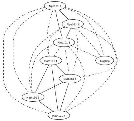
Figure 2: The colouring component of a trivial instance of course timetabling: There are three courses, Juggling, Math101 and Algo101, with 1, 4 and 3 events respectively. One group of students attends both Math101 and Algo101, another group attends both Juggling and Algo101, and events attended by a group of students cannot overlap in time. Each vertex in the associated conflict graph represents an event and there is an edge between two vertices, if the two corresponding events cannot take place concurrently. The edge is dashed, if this requirement is given by the enrolment of a student in both courses.

2.2 The Udine Course Timetabling Problem

The Udine Course Timetabling problem studied in this paper is maintained by Di Gaspero and Schaerf (2003) at Università degli studi di Udine. There are two important assumptions:

• Events are partitioned into disjoint subsets, called courses; events of any one course have to take place at different times, are attended by the same number of students, and are freely interchangeable

• A small number of distinct, possibly overlapping, sets of courses, representing enrolments prescribed to various groups of students, are identified and referred to as curricula.

Due to the second assumption, this problem is often referred to as “curriculum based timetabling”, as opposed to “student enrolment based timetabling”, which tries to minimise the number of conflicts among a possibly large number of enrolments. See Figure 2 for an illustrative example. The complete input can be captured by seven constant sets and eight mappings:

• $\operatorname{C}$, $\operatorname{U}$, $\operatorname{T}$, $\operatorname{R}$, $\operatorname{D}$, $\operatorname{P}$ are sets of courses, curricula, teachers, rooms, days, and periods, respectively

• $\textnormal{$\tilde{U}$}^{u}$ is the non-empty set of courses in curriculum $u$

• $\operatorname{N}$ is a subset of $\operatorname{C}\times\operatorname{P}$, giving forbidden course-period combinations

• $\textnormal{E}^{c}$ is the number of events course $c$ has in a week

• $\textnormal{S}^{c}$ is the number of students enrolled in course $c$

• $\textnormal{Q}^{c}$ is the prescribed minimum number of distinct week-days of instruction for course $c$

• $\textnormal{$\tilde{T}$}^{t}$ is the subset of courses $\operatorname{C}$ taught by teacher $t$

• $\textnormal{A}^{r}$ is the capacity of room $r$

• $\textnormal{$\tilde{D}$}^{d}$ is the subtuple (ordered subset) of $\operatorname{P}$ corresponding to periods in day $d$

• $\operatorname{W}$ is a vector of non-negative weights $(\operatorname{W^{RCap}},\operatorname{W^{TSpr}},\operatorname{W^{TCom}},\operatorname{W^{RStb}})$ for the four soft constraints described below.

Table 1: Instances of the Udine Course Timetabling problem: numbers of rooms and periods; the number of courses and the sum of their events in a week; frequency, or the portion of period-room slots in use, and utilisation, or the portion of period-seat slots in use (Beyrouthy et al., 2007); the number of distinct enrolments (“curricula”); numbers of edges and density in conflict graphs (CG) with vertices representing courses, rather than events (Burke et al., 2007).

Instance	AKA	Rooms	Periods	Courses	Events	Frequency (used slots)	Utilisation (used seats)	Curricula	Edges in CG (course-based)	Density of CG (course-based)
comp01	Fis0506-1	6	30	30	160	88.89 %	45.98 %	14	53	12.18 %
comp02	Ing0203-2	16	25	82	283	70.75 %	46.28 %	70	401	12.07 %
comp03	Ing0304-1	16	25	72	251	62.75 %	38.30 %	68	342	13.38 %
comp04	Ing0405-3	18	25	79	286	63.56 %	33.22 %	57	212	6.88 %
comp05	Let0405-1	9	36	54	152	46.91 %	43.50 %	139	917	64.08 %
comp06	Ing0506-1	18	25	108	361	80.22 %	45.28 %	70	437	7.56 %
comp07	Ing0607-2	20	25	131	434	86.80 %	41.71 %	77	508	5.97 %
comp08	Ing0607-3	18	25	86	324	72.00 %	37.39 %	61	214	5.85 %
comp09	Ing0304-3	18	25	76	279	62.00 %	32.67 %	75	251	8.81 %
comp10	Ing0405-2	18	25	115	370	82.22 %	36.38 %	67	481	7.34 %
comp11	Fis0506-2	5	45	30	162	72.00 %	56.23 %	13	75	17.24 %
comp12	Let0506-2	11	36	88	218	55.05 %	35.06 %	150	1181	30.85 %
comp13	Ing0506-3	19	25	82	308	64.84 %	38.14 %	66	216	6.50 %
comp14	Ing0708-1	17	25	85	275	64.71 %	34.78 %	60	368	10.31 %

Informally, the goal is to produce a mapping from events to period-rooms pairs such that:

1. For each course $c$, $\textnormal{E}^{c}$ events are timetabled

2. No two events take place in the same room in the same period

3. No two events of a single course, no two events taught by a single teacher, and no two events included in a single curriculum are taught at the same time

4. No event of course $c$ is taught in a period $p$, if $\left\langle{c,p}\right\rangle$ is in $\operatorname{N}$

5. The objective is to minimise a weighted sum of penalty terms

   $$\operatorname{W^{RCap}}\operatorname{P^{RCap}}+\operatorname{P^{TSpr}}\operatorname{W^{TSpr}}+\operatorname{P^{TCom}}\operatorname{W^{TCom}}+\operatorname{P^{RStb}}\operatorname{W^{RStb}},$$

   where:

   • $\operatorname{P^{RCap}}$ (for “room capacity”) is the number of students left without a seat at an event, summed across all events; this is the value of the number of students attending an event minus the capacity of the allocated room over all events where the value is positive

   • $\operatorname{P^{TSpr}}$ (for “spread of events of a course over distinct week-days”) sums the value of the number of prescribed distinct week-days of instruction minus the actual number of distinct week-days of instruction over all courses where the value is positive

   • $\operatorname{P^{TCom}}$ (for “time compactness”) is the number of isolated events in daily timetables of individual curricula; “[f]or a given curriculum we account for a violation every time there is one lecture not adjacent to any other lecture on the same day” (Di Gaspero et al., 2007)

   • $\operatorname{P^{RStb}}$ (for “room stability”) is the number of distinct course-room allocations on the top of a single course-room allocation per course.

In the original paper of Di Gaspero and Schaerf (2003), there were described only four instances of the Udine Course Timetabling Problem of up to 252 events and 57 distinct enrolments, with $(\operatorname{W^{RCap}},\operatorname{W^{TSpr}},\operatorname{W^{TCom}},\operatorname{W^{RStb}})=(1,5,2,0)$. Fourteen more instances of up to 434 events and 81 distinct enrolments have now been made available in Track 3 of the International Timetabling Competition, with weights $(\operatorname{W^{RCap}},\operatorname{W^{TSpr}},\operatorname{W^{TCom}},\operatorname{W^{RStb}})=(1,5,2,1)$. Their dimensions are summarised in Table 1.

2.3 An Integer Programming Formulation

Formally, the Udine Course Timetabling problem can be described using an integer programming model. Doing so necessitates the choice of decision variables. This is of little importance if the sole purpose is to formulate the problem formally, but becomes of paramount importance, if the performance of the formulation is evaluated. It seems tempting to see the problem as a variation of the three-index assignment and to use binary variables for each event-room-period combination. This corresponds to the trivial formulation of graph colouring, where the number of binary variables is the product of the number of vertices and an upper bound on the number of colours. There are, however, many alternative formulations of graph colouring (Burke et al., 2007) and it seems reasonable to use the best available formulation of graph colouring that would admit formulation of the soft constraints. After exploring a number of such alternatives, Burke et al. (2007) proposed a formulation based on a suitable clique-partition, which is given implicitly in many graph colouring applications. For Udine Course Timetabling, this formulation translates to a smaller number of “core” binary decision variables $x$, given by the product of the numbers periods, rooms, and courses, rather than events. Outside of those, there are dependent variables $v$, $q$, $z$, and $y$, whose values are derived from the values of $x$ in the process of solving:

• $x$ are binary decision variables indexed with periods, rooms and courses. Their values are constrained so that in any feasible solution, course $c$ should be taught in room $r$ at period $p$, if and only if $x_{p,r,c}$ is set to one.

• $v$ are binary decision variables indexed with courses and days. Their values are constrained so that in any feasible solution, there is at least one event of course $c$ held on day $d$, if and only if $v_{d,c}$ is set to one.

• $q$ are integer decision variables indexed with courses, whose values are bounded below by zero and above by the number of days in a week. Their values are constrained so that in any feasible solution, $q_{c}$ is the number of days course $c$ is short of the recommended days of instruction, $\textnormal{Q}^{c}$.

• $z$ are binary decision variables indexed with curricula, days, and an index-set $\operatorname{Z}$ of natural pattern-penalising constraints. Their values are constrained so that in any feasible solution, $z_{u,d,s}$ is set to one if and only if the pattern-penalising constraint indexed by $s\in\operatorname{Z}$ is violated in the timetable for curriculum $u$ and day $d$ given by the solution.

• $y$ are binary decision variables indexed with rooms and courses. Their values are constrained so that in any feasible solution, $y_{r,c}$ is set to one if and only if room $r$ is used by course $c$.

The objective function can be expressed as:

$$\min \;\operatorname{W^{RCap}}\sum_{r\in\operatorname{R}}\sum_{p\in\operatorname{P}}\sum_{\begin{subarray}{c}c\in\operatorname{C}\\ \textnormal{S}^{c}>\textnormal{A}^{r}\end{subarray}}x_{p,r,c}\;(\textnormal{S}^{c}-\textnormal{A}^{r})+\;\operatorname{W^{TCom}}\sum_{u\in\operatorname{U}}\sum_{d\in\operatorname{D}}\sum_{s\in\operatorname{Z}}z_{u,d,s}$$

$$+ \;\operatorname{W^{TSpr}}\sum_{c\in\operatorname{C}}q_{c}+\;\operatorname{W^{RStb}}\sum_{c\in\operatorname{C}}\left({\left({\sum_{r\in\operatorname{R}}y_{r,c}}\right)-1}\right)$$

Hard constraints can be formulated as follows:

$$\hskip 56.9055pt\forall c\in\operatorname{C}\hskip 56.9055pt \sum_{p\in\operatorname{P}}\sum_{r\in\operatorname{R}} x_{p,r,c} =\textnormal{E}^{c}$$ (1)

$$\hskip 56.9055pt\forall p\in\operatorname{P}\forall r\in\operatorname{R}\hskip 56.9055pt \sum_{c\in\operatorname{C}} x_{p,r,c} \leq 1$$ (2)

$$\hskip 56.9055pt\forall p\in\operatorname{P}\forall c\in\operatorname{C}\hskip 56.9055pt \sum_{r\in\operatorname{R}} x_{p,r,c} \leq 1$$ (3)

$$\hskip 56.9055pt\forall p\in\operatorname{P}\forall t\in\operatorname{T}\hskip 56.9055pt \sum_{r\in\operatorname{R}}\sum_{c\in\textnormal{$\tilde{T}$}^{t}} x_{p,r,c} \leq 1$$ (4)

$$\hskip 56.9055pt\forall p\in\operatorname{P}\forall u\in\operatorname{U}\hskip 56.9055pt \sum_{r\in\operatorname{R}}\sum_{c\in\textnormal{$\tilde{U}$}^{u}} x_{p,r,c} \leq 1$$ (5)

$$\hskip 56.9055pt\forall\left\langle{c,p}\right\rangle\in\operatorname{N}\hskip 56.9055pt \sum_{r\in\operatorname{R}} x_{p,r,c} =0$$ (6)

Constraint (1) enforces a given number of events to be taught for each course. Constraint (2) ensures no two events are taught in a single room at a single period. Constraints (3–5) stipulate that only one event within a single course or curriculum, or taught by a single teacher can be held at any given period. Notice the similarity of constraints (1–5) and the clique-based formulation of bounded graph colouring (Burke et al., 2007). Finally, constraint (6) forbids the use of some periods in timetables of some courses, corresponding to a pre-colouring extension. Notice also that constraint (5) renders constraint (3) redundant, if there are no courses outside of any curricula.

The formulation of soft constraints is less trivial and, as will be shown in Section 7 and Table 4, the formulation presented below proves to be quite challenging for modern general purpose integer programming solvers, even after the strengthening proposed by Burke et al. (2008a). Values of $v$ are forced to maxima of certain subsets of $x$ using constraints (7–8), in effect constructing daily timetables for individual curricula. Subsequently, the number of distinct week-days of instruction that course $c$ is short of the prescribed value $\textnormal{Q}^{c}$, can be forced into $q_{c}$ using constraint (9):

$$\hskip 56.9055pt\forall c\in\operatorname{C}\forall d\in\operatorname{D}\forall p\in\textnormal{$\tilde{D}$}^{d} \hskip 56.9055pt\sum_{r\in\operatorname{R}}x_{p,r,c} \leq v_{d,c}$$ (7)

$$\hskip 56.9055pt\forall c\in\operatorname{C}\forall d\in\operatorname{D} \hskip 56.9055pt\sum_{r\in\operatorname{R}}\sum_{p\in\textnormal{$\tilde{D}$}^{d}}x_{p,r,c} \geq v_{d,c}$$ (8)

$$\hskip 56.9055pt\forall c\in\operatorname{C} \hskip 56.9055pt\sum_{d\in\operatorname{D}}v_{d,c} \geq\textnormal{Q}^{c}-q_{c}$$ (9)

The “natural” formulation of penalisation of patterns (Burke et al., 2008b) occurring in daily timetables of individual curricula goes through the daily timetables bit by bit, first by checking isolated events in the first and the last period of the day, and later looking for triples of consecutive periods with only the middle period occupied by an event: For an instance with four periods per day, this is:

$$\forall u\in\operatorname{U},d\in\operatorname{D},\forall\left\langle{p_{1},p_{2},p_{3},p_{4}}\right\rangle\in\textnormal{$\tilde{D}$}^{d} \;\sum_{c\in\textnormal{$\tilde{U}$}^{u}}\sum_{r\in\operatorname{R}} (x_{p_{1},r,c}-x_{p_{2},r,c}) \leq z_{u,d,1}$$ (10)

$$\forall u\in\operatorname{U},d\in\operatorname{D},\forall\left\langle{p_{1},p_{2},p_{3},p_{4}}\right\rangle\in\textnormal{$\tilde{D}$}^{d} \;\sum_{c\in\textnormal{$\tilde{U}$}^{u}}\sum_{r\in\operatorname{R}} (x_{p_{4},r,c}-x_{p_{3},r,c}) \leq z_{u,d,2}$$ (11)

$$\forall u\in\operatorname{U},d\in\operatorname{D},\forall\left\langle{p_{1},p_{2},p_{3},p_{4}}\right\rangle\in\textnormal{$\tilde{D}$}^{d} \;\sum_{c\in\textnormal{$\tilde{U}$}^{u}}\sum_{r\in\operatorname{R}} (x_{p_{2},r,c}-x_{p_{1},r,c}-x_{p_{3},r,c}) \leq z_{u,d,3}$$ (12)

$$\forall u\in\operatorname{U},d\in\operatorname{D},\forall\left\langle{p_{1},p_{2},p_{3},p_{4}}\right\rangle\in\textnormal{$\tilde{D}$}^{d} \;\sum_{c\in\textnormal{$\tilde{U}$}^{u}}\sum_{r\in\operatorname{R}} (x_{p_{3},r,c}-x_{p_{2},r,c}-x_{p_{4},r,c}) \leq z_{u,d,4}$$ (13)

Just as for constraints (7–9), cuts strengthening constraints (10–13) were described by Burke et al. (2008a). Finally, values of $y$, similar to values of $v$, are forced to maxima of certain subsets of $x$:

$$\hskip 56.9055pt\forall p\in\operatorname{P}\forall r\in\operatorname{R}\forall c\in\operatorname{C} \hskip 56.9055ptx_{p,r,c} \leq y_{r,c}$$ (14)

$$\hskip 56.9055pt\forall r\in\operatorname{R}\forall c\in\operatorname{C} \hskip 56.9055pt\sum_{p\in\operatorname{P}}x_{p,r,c} \geq y_{r,c}$$ (15)

These constraints complete the formulation, which will be later referred to as Monolithic.

2.4 How Difficult is this for Exact Solvers?

One might hope that it is enough to pass this formulation to a modern integer programming solver and wait. After all, integer programming has been used in timetabling ever since Lawrie (1969) generated feasible solutions to a school timetabling problem using a branch and bound procedure with Gomory cuts. Tripathy (1984) and Carter (1989) solved instances of a course timetabling problem of up to 287 events with several soft constraints using Lagrangian relaxation. They have not, however, introduced any constraints penalising interaction between events in timetables other than, of course, straightforward conflicts. More recently, a number of modest instances of course timetabling problems have been tackled using off-the-shelf solvers, without introducing any new cuts (Dimopoulou and Miliotis, 2004; Qualizza and Serafini, 2005; Daskalaki et al., 2004, 2005; Mirhassani, 2006). For instance, Daskalaki et al. (2004, 2005) solved instances of up to 211 events using ILOG CPLEX. Of special interest are studies by Al-Yakoob and Sherali (2007) and Schimmelpfeng and Helber (2007), who have modelled a larger number of constraints. In the most rigorous study so far, Avella and Vasil’ev (2005) presented a branch-and-cut solver for the Benevento Course Timetabling Problem, which forbids some interactions of events in timetables other than conflicts using hard constraints. In this setting, Avella and Vasil’ev (2005) have been able to solve instances of up to 233 events and 14 distinct enrolments, but conceded that application of their solver to the four small instances of Udine Course Timetabling available in 2005 yielded “poor results”. In Udine Course Timetabling, such interactions are penalised by soft constraints (7–15), which (it turns out) make the problem considerably more difficult. Several integer programming formulations of the problem have been studied by Burke et al. (2007, 2008b), and more recently by Lach and Lübbecke (2008a, b). Both approaches can now solve the original instances of Udine Course Timetabling from 2005, but optimal solutions to instances from the International Timetabling Competition 2007, or optima for large real-life instances of university course timetabling problems are, as it seems, out of reach, so far.

In particular, it seems that it is the run-time of the linear programming (LP) solver that is prohibitive to progress on more difficult instances from the International Timetabling Competition (ITC) using the Monolithic formulation. For relatively easier instances (comp01 and comp11 from ITC 2007), root relaxation obtained from Monolithic takes less than thirty seconds to solve using the default ILOG CPLEX 11 Dual Simplex LP Solver and the search proceeds swiftly. On the remaining instances, however, the root relaxation is far more expensive, taking up to 6489 seconds on comp07. For complete results obtained using the CPLEX 11 Dual Simplex LP Solver, see Table 4. Informal evidence suggests that run times of both the CPLEX 11 Barrier and the CPLEX 11 Primal Simplex LP solvers are shorter, whereas run-times of either SoPlex (Wunderling, 1996) and CLP (Forrest et al., 2004) are longer. Hence, it is not particularly surprising that for most instances (all except from comp01, comp05, and comp11), CPLEX Mixed Integer Programming (MIP) solver using Monolithic and default settings does not produce any feasible solution within 40 CPU units, branching at the speed of ten to thirty nodes per hour. This can hardly be described as satisfactory progress.

Although the total run-time or time spent at the root node may not be of particular importance, as long as the instance is solved close to optimality within a reasonable time limit, for example over a weekend, relying on robustness of modern solvers does not seem to be an option for real-life instances (Murray et al., 2007). First, such instances are often many times larger than those used in the International Timetabling Competition 2007, including comp07. Second, their formulations are considerably more complex and tend to change over time, whereas the behaviour of general solvers on monolithic formulations tends to be rather difficult to predict, with run-time often rising rapidly on addition of seemingly trivial constraints. Finally, general solvers only seldom perform in the “anytime” fashion of Zilberstein (1996) on monolithic formulations, which would make it possible to obtain a solution whenever the solver is stopped. It thus makes sense to study decompositions of the problem and the performance of heuristic methods based on them.

3 Multiphase Exploitation of Multiple Objective-/Value-restricted Submodels (MEMOS)

In short, our approach can be seen as a hybridisation of loosely coupled integer programming solvers working on very different sub-problems of similar difficulty. Each solver is, time-limit permitting, exact within the given search space, and together, the solvers provide heuristic solutions with global lower bounds. It seems, however, useful to set this description in the broader context of hybrid metaheuristics, even if this still seems difficult to do precisely, but concisely, despite the numerous attempts (Calégari et al., 1999; Puchinger and Raidl, 2005; El-Abd and Kamel, 2005; Raidl, 2006) to develop a taxonomy of the field.

3.1 Hybridisation

Hybridisation can clearly occur in two different fashions:

• Algorithm hybridisation, using multiple algorithms for the same problem

• Formulation hybridisation, using multiple subproblems or multiple levels of abstraction

Although, in theory, hybridisation can occur in both fashions, in practice, heuristics often exploit only algorithm hybridisation: Multiple algorithms producing solutions to the complete problem, with or without a feasible solution on the input. A typical example of algorithm hybridisation is the “construct-improve” scheme, which is a standard practice in metaheuristic solvers. A constructive algorithm is used in order to produce one, or many, different initial solutions, which are then improved using some variant of local search. See the concise overview by Blum and Roli (2003) for details. Embedding of multiple primal and improvement heuristics (Fischetti and Lodi, 2003; Danna et al., 2005; Berthold, 2007b) in general integer programming solvers can be seen as another example of algorithm hybridisation. In contrast, the deliberate creation and exploitation of multiple sub-problems, restricted to certain components in the objective function, with certain values fixed, or both, seems underutilised.

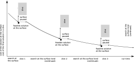
Figure 3: A schematic illustration of the data flows in the metaheuristic.

3.2 Submodels

The critical point in our approach is precisely that: sub-problems solved at various stages are different, although possibly overlapping. That is, we create sub-problems using combinations of

• Value-Restrictions: Fix the values of a subset of the variables, distance from a solution with respect to Hamming distance ($L_{0}$ norm), or sums across subsets of variables. This is a standard method to generate a neighbourhood.

• Objective-Restrictions: Suppose that we have a minimisation problem and some penalty term $P^{R}$ is part of the objective, with associated weight $W^{R}$. We then use one of two options:

  • Objective-Ignore-Term We drop all consideration of the penalty – this corresponds to setting $W^{R}=0$.

  • Objective-Fix-Term We force $P^{R}=0$. This converts the penalty to a hard constraint.

  The objective restriction might loosely be thought of as the dual of the variable restrictions.

In any case, the intent is that the restriction will give a sub-problem that can be significantly simplified compared to the full problem, and of comparable difficulty to other problems obtained in the decomposition.

This can be illustrated on a class of problems, which often occurs in Scheduling and Timetabling applications, where there is a graph colouring component expanded over another dimension. Imagine for example the assignment of jobs to time-periods, expanded over machines, or the assignment of events to time-periods, expanded over rooms. In such cases, only one part of the objective is usually related to the expanded problem, whereas the rest is related to the graph colouring component. This results in structures such as: such as:

$$\min\left(\sum_{i=1}^{n}c_{i}x_{i}+\sum_{j=1}^{o}d_{j}\max_{k\in I_{j}}x_{k}+\sum_{l=o+1}^{p}d_{l}\max(f(l,\max_{m\in I_{l}}x_{m}),0)\right)$$ (16)

$$\max_{k\in I_{j}}x_{k}\leq 1\;\forall j\in\{1,2,\ldots,o\}$$ (17)

$$Ax\geq b$$ (18)

$$x\in\{0,1\}^{n}$$ (19)

where $n$, $m$, $o$, and $p$ are integral constants, $x$ is a vector of $n$ integral decision variables, $A$ is an $n\times m$ constant matrix, $b$, $c$, and $d$ are compatible constant vectors, and for each $j=\{1,2,\ldots,p\}$, $I_{j}$ is a subset of $\{1,2,\ldots,n\}$. Notice that the second two terms in the objective function, weighted by $d$, are related only to the graph colouring component, and necessitate implementation of the $\max$ function using additional variables. The number of “core” variables $x$ can be much less than the number of additional variables implementing the $\max$ function over various subsets of $x$. Hence, it makes sense to use the restricted objective:

$$\min\left(\sum_{j=1}^{o}d_{j}\max_{k\in I_{j}}x_{k}+\sum_{l=o+1}^{p}d_{l}\max(f(l,\max_{m\in I_{l}}x_{m}),0)\right),$$ (20)

ignoring the first term in the original objective (16). Given the constraint matrix $A$ exhibit certain structure (17), this should allow for aggregation of $n$ variables $x$ into $o$ variables $y$:

$$\min\left(\sum_{j=1}^{o}d_{j}y_{j}+\sum_{l=o+1}^{p}d_{l}\max(f(l,y_{g(l)}),0)\right)A^{\prime}y\geq b^{\prime}$$ (21)

$$y\in\{0,1\}^{o}$$ (22)

where $g$ is a suitable mapping. Notice that some constraints may have to be relaxed in deriving the new constraints ($A^{\prime}b^{\prime}$) from the original ones ($Ab$). In Table 1 and below, we denote such a subproblem as “surface”. Such an objective-restricted subproblem, however, should solve considerably faster than the original problem (16–19).

Once a solution to the objective-restricted subproblem is found, it makes sense to resolve the original problem (16–19) with the additional constraints:

$$\max_{k\in I_{j}}x_{k}=y_{j} \;\;\;\forall j\in\{1,2,\ldots,o\}$$ (23)

$$\max(f(l,\max_{m\in J_{l}}x_{m})=y_{l} \;\;\;\forall l\in\{o+1,o+2,\ldots,p\}.$$ (24)

In Table 1 and below, we denote such subproblems as “dives”. This should result in considerable reductions of the model in presolving, and consequently in value-restricted subproblems which solve considerably faster than the original problem (16–19).

One can also use any combination of these, and could also separately treat different terms of the objective. This is, however, limited by the availability of a decomposition into such sub-problems, given by the structure of a solution and the objective, applicable reformulations, and our ability to automate their execution. For many “academic” problems there tends to be just a single term on the objective – for example, for the TSP we have only the tour length, and the objective restriction is hence not relevant. For many real-life problems, however, it is quite likely that the solution has a more complex structure, and there are multiple soft constraints corresponding to multiple penalty terms in the objective. University course timetabling (Murray et al., 2007) as opposed to pure graph colouring, or vehicle routing problems (Chabrier, 2006; Pisinger and Røpke, 2007) as opposed to the travelling salesman problem, provide good examples of possible application areas. In this case ignoring or fixing some terms can give significantly easier problems, yet still provide enough information to guide solution of the full problem. As we will see, automated preprocessing in-built in modern integer programming solvers is often too weak, and we do need to apply non-automatic reformulations “by-hand”. Ultimately, our work is directed towards automating decompositions and reformations of such problems with “multiple soft constraints”, exploiting cases in which the objectives can have differing levels of importance.

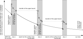
Figure 4: A schematic illustration of information flows in the anytime algorithm: feasible solutions at the surface are transformed into neighbourhoods for dives, executed immediately. Upper bounds (costs of best-so-far solutions) are being carried over from dive to dive.

3.3 Control Strategies

Another important and often neglected question in the design of hybrid metaheuristics asks for the sequence of periods of searching at the surface and periods of diving in neighbourhoods, sometimes referred to as “the control strategy” (Puchinger and Raidl, 2005; Raidl, 2006). Very often, a variant of the anytime algorithm (Zilberstein, 1996) is used, perhaps because it fits well into the large neighbourhood search scheme. There are, however, two obvious alternatives of the producer-consumer relationship:

• Anytime algorithm: search at the surface and dives are interleaved and dives are perfomed as soon as suitable feasible solutions are found. The algorithm is parametrised with the types of dives performed, their order, and possibly the onset of execution of each type. See also Figure 4.

• Contract algorithm: search at the surface is carried out for a certain time and only then are the dives performed, firstly ordered by dive type with the least expensive dives coming first, and secondly ordered in the ascending order of the cost (in minimisation problems) of the solution at the surface the dive is derived from. Hence, the algorithm is parametrised with the types of dives performed, the time limit and the proportion of the time limit spent at the surface. See also Figure 5.

It seems that, in practice, a time-limit is often given and considerable performance improvements can be gained from exploiting this in a Contract algorithm. If the neighbourhoods can be searched in the ascending order of the cost of the solution at the surface and the cost of the present-best solution found in dives is applied as an upper bound in all dives except the first one, a considerable number of dives can be cut off immediately and the algorithm needs not to be parametrised with the onset of diving. (This is suggested in Figure 5.) Notice that the ascending order of the cost corresponds to the inverse order of the time of discovery, if we are producing only progressively improving solutions at the surface.

Generally, such Multiphase Exploitation of Multiple Objective-/value-restricted Submodels (MEMOS) will no longer be complete or exact. The intention is, however, to produce good solutions quickly.

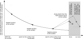
Figure 5: A schematic illustration of the contract algorithm: dives of all types are postponed until the surface search finishes (runs out of time), when they are carried out in the descending order of the time of discovery of the neighbourhood, with the upper bound found from in the best neighbourhood often cutting off the dives into other neighbourhoods as soon as their local lower bounds are established.

4 MEMOS for Udine Course Timetabling

In the design of the particular MEMOS heuristic, we need to make specific decisions as to which sub-problems the “surface” and “dive” components need to solve. In doing so, it seems useful to think of the problem from the multi-objective perspective. In the Udine Course Timetabling problem introduced in Section 2, a given set of weights is used to linearise the penalties given by the number of violations of four soft constraint (“objectives”) into a single-objective problem. The four objectives are not necessarily linked, however. The formulation introduced in Section 2.3 models the four soft constraints one-by-one, each objective using a separate subset of constraints and a separate subset of variables derived from the main decision variables. Hence, it is natural to consider sub-problems arising from setting weights related to a subset of the four soft constraints to zero.

If some weights are set to zero, the corresponding objective can be ignored and the problem formulation can be simplified. Ideally, one would be able to rely upon the preprocessing in-built in an integer programming solver to do this. As suggested by Table 3, however, present-day general purpose integer programming solvers are not particularly effective for such major reformulations. Non-automatic reformulation can, however, result in much faster relaxations, outside of having other desirable properties (Trick, 2005). In our case, such a desirable property might be the ease of conversion of solutions obtained at the “surface” to neighbourhoods for the dives. As suggested in Table 4, a careful choice of the decomposition and manual reformulation can lead to the run-time of the linear programming solver at the relaxation either in the surface component or within a dive being cut by factor of more than two thousand, compared to the “monolithic” formulation.

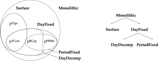
Figure 6: A schematic illustration of the penalties considered in the formulations we use: Monolithic uses the complete objective function, Surface sets $\operatorname{W^{RCap}}=\operatorname{W^{RStb}}=0$, DayFixed has $\operatorname{P^{TSpr}}$ fixed, PeriodFixed has $\operatorname{P^{TSpr}}$ and $\operatorname{P^{TCom}}$ fixed, and DayDecomp has $\operatorname{P^{TSpr}}$ fixed and $\operatorname{W^{RStb}}=0$.

4.1 Objective-restricted Submodels

One could consider generating reduced problems by setting any subset of the weights to zero. With four penalties, there are $2^{4}-1=15$ possible non-trivial choices. However, we only use the following problem:

• Surface: We set $\operatorname{W^{RCap}}=\operatorname{W^{RStb}}=0$ so that room over-filling and room stability are not considered. Since no explicit room assignments are required, there can be much fewer variables. We will see later that the ternary variables $x_{p,r,c}$ are no longer required, which gives us much shorter run-times of the linear programming solver. (See Table 4.) However, we add extra constraints that bound the number of rooms used in any single period; they impose that there will always be enough rooms for courses at each period, and so guarantee that a surface solution can always be extended by the dive to a feasible solution to the full problem. However, these extra constraints convert the colouring to bounded colouring and make solving the “surface” search harder, both in theory and practice.

The sets of the objectives considered by each formulation are illustrated in Figure 6. This also serves to emphasise the crucial point that the methods we use are intended for the case of multiple terms in the objective, or equivalently, for multiple classes of relatively-complex soft constraints.

One can reasonably ask why we use this particular split between surface and dive models. Firstly, the graph colouring component is important in the instances under consideration. In Table 1, we can see that the ratio of events to available room slots is typically 60-90% which is quite high, so it is reasonable that the bounded colouring problem is hard so solve, and so ought to be solved first. That is, the bounded colouring needs to be done at the surface level. Also, Table 3 gives optimal objective vectors for different weight vectors. (It does this for the small instance comp01 that happens to be fairly easy to solve exactly, and uses the monolithic IP formulation detailed in the previous section.) We see that the time-related penalties ($\operatorname{P^{TSpr}}$ and $\operatorname{P^{TCom}}$) make the largest contributions to the final objective, and so it is natural to address these first. Limited experimentation has been conducted with solvers where $\operatorname{W^{RCap}}=\operatorname{W^{RStb}}=\operatorname{W^{TCom}}=0$. As is suggested by Table 3, the solver at the surface is not considerably faster, when only automatic reductions are considered. Rather surprisingly, the solver is not considerably faster, however, even when non-automatic reformulations are applied, and these gains do not offset the need to spend more time diving. (See Section 5.2.) There are also alternatives exploiting interchangeable rooms.

Table 2: The effects of disabling various subsets of soft constraints by setting the corresponding weights in the monolithic model to zero on CPLEX 10 run-time for instance comp01. Only the default in-built pre-processing and cuts are used and only the best feasible solution obtained within one hour per run is presented. Notice that when a weight is set to zero, the associated penalty is typically high.

$\operatorname{W^{RCap}}$	$\operatorname{W^{TSpr}}$	$\operatorname{W^{TCom}}$	$\operatorname{W^{RStb}}$	LP Matrix	Barrier LP Runtime	Node with last feas. sol.	Default IP Runtime	$\operatorname{P^{RCap}}$	$\operatorname{P^{TSpr}}$	$\operatorname{P^{TCom}}$	$\operatorname{P^{RStb}}$	Obj.
0	0	0	0	$6639\times 5407$	44.08 s	0	66 s	2294	30	350	93	0
0	0	0	1	$6639\times 5407$	43.66 s	370	1066 s	2706	30	350	0	0
0	0	2	0	$7059\times 5757$	61.24 s	140	884 s	2107	30	0	77	0
0	5	0	0	$6665\times 5435$	40.44 s	0	148 s	2387	0	350	92	0
1	0	0	0	$6639\times 5407$	21.68 s	0	62 s	4	30	350	44	4
0	0	2	1	$7059\times 5757$	67.73 s	617	1033 s	2874	30	0	0	0
0	5	0	1	$6665\times 5435$	39.41 s	402	1554 s	2023	0	350	0	0
0	5	2	0	$7085\times 5785$	66.18 s	90	881 s	2365	0	0	78	0
1	0	0	1	$6639\times 5407$	9.97 s	180	521 s	4	30	350	1	5
1	0	2	0	$7059\times 5757$	21.21 s	124	518 s	4	30	0	31	4
1	5	0	0	$6665\times 5435$	10.01 s	0	52 s	4	0	350	44	4
0	5	2	1	$7085\times 5785$	39.50 s	1964	1050 s	1672	0	0	0	0
1	0	2	1	$7059\times 5757$	21.40 s	487	1416 s	4	30	0	1	5
1	5	0	1	$6665\times 5435$	7.96 s	269	651 s	4	0	350	1	5
1	5	2	0	$7085\times 5785$	22.35 s	145	395 s	4	0	0	43	4

Table 3: The effects of varying the weight $\operatorname{W^{TSpr}}$ on CPLEX 10 run-time for the monolithic model and instance comp01.

$\operatorname{W^{RCap}}$	$\operatorname{W^{TSpr}}$	$\operatorname{W^{TCom}}$	$\operatorname{W^{RStb}}$	LP Matrix	Barrier LP Runtime	Node with last feas. sol.	Default IP Runtime	$\operatorname{P^{RCap}}$	$\operatorname{P^{TSpr}}$	$\operatorname{P^{TCom}}$	$\operatorname{P^{RStb}}$	Obj.
1	2	2	1	$7085\times 5785$	19.19 s	1053	1205 s	4	0	0	1	1
1	4	2	1	$7085\times 5785$	19.19 s	405	$>3600$ s	4	0	0	2	(6)
1	8	2	1	$7085\times 5785$	19.49 s	1420	$>3600$ s	5	0	0	1	(6)
1	16	2	1	$7085\times 5785$	19.23 s	4822	$>3600$ s	4	0	0	2	(6)
1	32	2	1	$7085\times 5785$	19.06 s	586	$>3600$ s	4	0	0	2	(6)
1	64	2	1	$7085\times 5785$	19.39 s	3803	2387 s	4	0	0	1	5

4.2 Exploiting Interchangeable Rooms: “Multi–rooms”

Suppose that we have two rooms of exactly the same size. Then the only way that the rooms are not interchangeable is because of the room stability constraint. If we take a solution and swap the rooms at any single time period then no constraints are broken and no objectives affected, except potentially the room stability. Hence, if we are using a formulation, such as the surface, that does not care about room stability, then we can treat the rooms as interchangeable. Thus, we could replace the 2 standard rooms with a single room with multiplicity, which we call a “multi-room”.

A multi-room of size “($m$,$a$)” will have multiplicity $m$, capacity $a$, and will function exactly as $m$ separate indistinguishable rooms. That is: It can accommodate $m$ separate events of sizes up to $a$ each, without any overflow. This mild extension is straightforward, but has the advantage that we then have the option to replace the $r$ index of the $x_{p,r,c}$ variables by an index into a set of multi-rooms. Any solution using multi-rooms can be translated into constraints on original rooms that define a neighbourhood in the full problem. Within this neighbourhood, there will always be a feasible solution, and we can easily find the one minimising $\operatorname{P^{RStb}}$, the penalty for “room stability”.

Here we use multi-rooms only as a device to reduce the number of variables and remove symmetries that would enlarge the search space. However, it is also reasonable that multi-rooms could be directly useful. Specifically, in practice, the room stability might well not be quite so strict as the Udine timetabling instances demand. In some teaching facilities, there could well be a suite of teaching rooms that are all of the same size, with the same facilities, and which are located very close to each other. In such a case, it could well be that there really would be no need for a room stability penalty for mixed use. In this case, they could well be treated exactly as a single multi-room with appropriate multiplicity.

Generally, only a few rooms do have exactly the same sizes. However, it is often the case that there are many rooms of roughly the same size. To exploit this situation, note that if we join two rooms of different sizes into a single multi-room then it can affect the room capacity objective, but again it will not affect the hard constraints. Hence, we do allow the creation of relaxations in which various sets of rooms are joined into associated multi-rooms with capacity the size of the largest original room. Specifically, if we select a set of multi-rooms with capacities $\{c_{i}|i=1\ldots\left|{\operatorname{R}}\right|\}$ then we can replace them with a multi-room of size $(m,\max c_{i}\}$. An intermedaite case would be to divide the rooms into two multi-rooms, according to whether they are smaller or not than some selected intermediate size. We will introduce such a neighbourhood generator, denoted by Surface2, in Section 5.

4.3 Value-restricted Submodels

For the dives, we use value-restricted submodels of the Monolithic model. Two pure value-restricted submodels are defined by restricting the times of courses based on the solution obtained at the surface level:

• PeriodFixed dives: The periods of all the courses are fixed to be the same as obtained from the surface solution.

• DayFixed dives: The days of all the courses are fixed, but not the explicit period within the day. That is, for each course the assigned “period” is relaxed to just give a day assignment.

In both pure value-restricted subproblems, the spread of events of a course over distinct week-days is entirely fixed, and $\operatorname{W^{TSpr}}$ hence becomes irrelevant. PeriodFixed dives also fix time compactness penalty $\operatorname{P^{TCom}}$, and thus only room assignment remains to be found, minimising the room related penalties ($\operatorname{P^{RCap}}$ and $\operatorname{P^{RStb}}$). In DayFixed dives, the compactness penalty $\operatorname{P^{TCom}}$ can still potentially be improved. A middle ground between these two approaches is offered by value- and objective-restricted submodels.

4.4 Value- and Objective-restricted Submodels

Two obvious value- and objective-restricted submodels can be defined by restricting the times of courses based on the solution obtained at the surface level, and not considering $\operatorname{P^{RStb}}$ or by forcing $\operatorname{P^{RStb}}$ to zero:

• DayDecomp dives: $\operatorname{P^{RStb}}$ is not considered and the days of all the courses are fixed, but not the explicit period within the day. That is, for each course, the assigned “period” is relaxed to just give a day assignment and the lowest possible penalty for time compactness and room capacity is sought.

• DayFixedZero$\operatorname{P^{RStb}}$ dives: $\operatorname{P^{RStb}}$ is forced to be zero and the days of all the courses are fixed, but not the explicit period within the day. That is, for each course, the assigned “period” is relaxed to just give a day assignment and an assignment with zero penalty for room stability is sought.

These two value- and objective-restricted submodels have the advantage that they reduce the links between variables representing individual days, which translates into matrices closer to the block structure and improvements in the performance of the diving integer programming solver. Many other subproblems, most notably variants of PeriodFixed and DayFixed dives using stochastic ruining (Schrimpf et al., 2000; Dueck et al., 2002), are of course possible, but are not studied here. Some experience with implementing and testing the presented alternatives empirically is described in Section 7.

4.5 Control Strategies

Finally, we have designed both Anytime and Contract control strategies for Udine Course Timetabling, using PeriodFixed dives followed by DayFixed dives. The details of their functioning is outlined in Figure 7. Contract algorithms turned out to perform better, as expected, especially when multiple solutions can be found at Surface within the given time limit. The only difficulty seems to be the choice of the partition of short time limits between Surface and dives in Contract algorithms. When a time limit is given, and is not too strict, however, there seem to be no reasons to use Anytime strategies.

class AnytimeStrategy implementing Strategy:

  constructor(config):

    keep track of config

    initialise bestSoFar to an error value

  onFeasibleSolution():

    foreach type in config.getDiveTypes():

      if time > config.getAnytimeDivingOnset(type):

        Neighbourhood def = getNeighbourhood(type)

        update bestSoFar with

          dive(def, config.getDiveTimeLimit(type))

  onTimeout():

    return bestSoFar

class ContractStrategy implementing Strategy:

  constructor(config):

    keep track of config

    initialise a stack of neighbourhoods n[t]

      for each t in config.getDiveTypes()

  onFeasibleSolution():

    foreach type in config.getDiveTypes():

      fixDayNeighbs.push(getNeighbourhood(type))

  onTimeout():

    initialise bestSoFar to an error value

    foreach type in config.getDiveTypes():

      c = 0

      while time > config.getTimelimit() &&

          ! n[type].empty() && c < config.getRunLimit(type):

        update bestSoFar with

          dive(n[type].pop(), config.getDiveTimeLimit(type))

        c += 1

class SampleAnytimeSolver():

  solve():

    config.setDiveTypes([FixPeriod, FixDay])

    foreach type in config.getDiveTypes():

      come up with a suitable time limit for type

      config.setDiveTimeLimit(type, limit)

    load an instance

    initialise a solver for Surface, instance, and config

    install AnytimeStrategy(config) as a solver callback

    try solving Surface

class SampleConstractSolver():

  solve(timeLimit):

    config.setTimeLimit(timeLimit)

    config.setDiveTypes([FixPeriod, FixDay])

    config.setDiveTimeLimit(FixPeriod, timeLimit/50)

    config.setDiveTimeLimit(FixDay, timeLimit/5)

    foreach type in config.getDiveTypes():

      config.setRunLimit(type, 3)

    load an instance

    initialise a solver for Surface, instance, and config

    install ContractStrategy(config) as a solver callback

    try solving Surface for timeLimit/3

Figure 7: Pseudocode of the control strategies in use

5 Non-Automatic Re-Formulations of the Subproblems

As has been described in Section 3, at the “surface” level of the heuristic for Udine Course Timetabling, there is an objective-restricted neighbourhood generator trying to find an assignment of events to periods, such that at most a given number of events takes place at any given period, but disregarding other issues of assignment of rooms, such as room capacities. Feasible solutions of the assignment of events to periods are relaxed into value-restricted neighbourhoods given by the assignment of events to days or periods. It would obviously be possible to use the monolithic formulation with weights $(\operatorname{W^{RCap}}\operatorname{W^{TSpr}}\operatorname{W^{TCom}}\operatorname{W^{RStb}})=(0,5,2,0)$ at the “surface” level, and to rely on the automatic pre-solving routines in a modern integer programming solver. As will be shown in Section 7, however, improvements in the run-time of the linear programming solver, which determine the run-time of the integer programming solver, of several orders of magnitude can be achieved by non-automatic reformulation.

5.1 The Search for Good Neighbourhoods

In the formulation that we denote as Surface, the “core” decision variables $w$ are accompanied by dependent variables $v$, $q$, and $z$, introduced previously:

• $w$ are binary decision variables indexed with periods and courses. Their values are constrained so that in any feasible solution, course $c$ should be taught at period $p$, if and only if $w_{p,c}$ is set to one.

The objective function can be expressed as:

$$\min\;\operatorname{W^{TCom}}\sum_{u\in\operatorname{U}}\sum_{d\in\operatorname{D}}\sum_{s\in\operatorname{Z}}z_{u,d,s}+\;\operatorname{W^{TSpr}}\sum_{c\in\operatorname{C}} q_{c}$$

Hard constraints can be formulated similarly to those in Monolithic:

$$\hskip 56.9055pt\forall c\in\operatorname{C}\hskip 56.9055pt \sum_{p\in\operatorname{P}} w_{p,c} =\textnormal{E}^{c}$$ (25)

$$\hskip 56.9055pt\forall p\in\operatorname{P}\forall u\in\operatorname{U}\hskip 56.9055pt \sum_{c\in\textnormal{$\tilde{U}$}^{u}} w_{p,c} \leq 1$$ (26)

$$\hskip 56.9055pt\forall p\in\operatorname{P}\forall t\in\operatorname{T}\hskip 56.9055pt \sum_{c\in\textnormal{$\tilde{T}$}^{t}} w_{p,c} \leq 1$$ (27)

$$\hskip 56.9055pt\forall p\in\operatorname{P}\hskip 56.9055pt \sum_{c\in\operatorname{C}} w_{p,c} \leq\left|{\operatorname{R}}\right|$$ (28)

$$\hskip 56.9055pt\forall\left\langle{c,p}\right\rangle\in\operatorname{N}\hskip 56.9055pt w_{p,c} =0$$ (29)

Notice that constraint (28) is the only mention of rooms in this formulation of neighbourhood definition. It makes the number of rooms used in any period smaller than $\left|{\operatorname{R}}\right|$, which corresponds to making the colouring bounded. It would be possible, for example, to constrain the number of large courses taught in any one period to be less than the number of large rooms, with suitable definitions of “large”. Similar constraints, however, do not seem to improve the quality of neighbourhoods significantly.

By minor changes of constraints (7–9) in the monolithic formulation, the array $q$ can be constrained using:

$$\hskip 56.9055pt\forall c\in\operatorname{C}\forall d\in\operatorname{D}\forall p\in\textnormal{$\tilde{D}$}^{d}\hskip 56.9055pt w_{p,c} \leq v_{c,d}$$ (30)

$$\hskip 56.9055pt\forall c\in\operatorname{C}\forall d\in\operatorname{D}\hskip 56.9055pt \sum_{p\in\textnormal{$\tilde{D}$}^{d}}w_{p,c} \geq v_{c,d}$$ (31)

$$\hskip 56.9055pt\forall c\in\operatorname{C}\hskip 56.9055pt \sum_{d\in\operatorname{D}}v_{c,d} \geq\textnormal{Q}^{c}-q_{c}$$ (32)

Inequalities 30 and 31 in effect aggregate values from $w$ into $v$. Inequality 32 then calculates the number of days the instruction is short of the recommended value in Q.

Patterns can be penalised again using the natural formulation, used already in constraints (10–13) in the monolithic model. For instances with four periods per day, we obtain:

$$\forall u\in\operatorname{U}d\in\operatorname{D}\forall\left\langle{p_{1},p_{2},p_{3},p_{4}}\right\rangle\in\textnormal{$\tilde{D}$}^{d} \sum_{c\in\textnormal{$\tilde{U}$}^{u}} (w_{p_{1},c}-w_{p_{2},c}) \leq z_{u,d,1}$$ (33)

$$\forall u\in\operatorname{U}d\in\operatorname{D}\forall\left\langle{p_{1},p_{2},p_{3},p_{4}}\right\rangle\in\textnormal{$\tilde{D}$}^{d} \sum_{c\in\textnormal{$\tilde{U}$}^{u}} (w_{p_{4},c}-w_{p_{3},c}) \leq z_{u,d,2}$$ (34)

$$\forall u\in\operatorname{U}d\in\operatorname{D}\forall\left\langle{p_{1},p_{2},p_{3},p_{4}}\right\rangle\in\textnormal{$\tilde{D}$}^{d} \sum_{c\in\textnormal{$\tilde{U}$}^{u}} (w_{p_{2},c}-w_{p_{1},c}-w_{p_{3},c}) \leq z_{u,d,3}$$ (35)

$$\forall u\in\operatorname{U}d\in\operatorname{D}\forall\left\langle{p_{1},p_{2},p_{3},p_{4}}\right\rangle\in\textnormal{$\tilde{D}$}^{d} \sum_{c\in\textnormal{$\tilde{U}$}^{u}} (w_{p_{3},c}-w_{p_{2},c}-w_{p_{4},c}) \leq z_{u,d,4}$$ (36)

This formulation of Surface can obviously also be strengthened by addition of cuts, as described by Burke et al. (2008a).

5.2 Better Neighbourhoods?

The approach outlined above is not the only possible neighbourhood generator, although the range of possible formulations is somewhat limited by the choice of decision variables. Considering further soft constraints would necessitate the addition of a considerable number of variables, resulting in very slow LP relaxations. (See Table 4 for an illustration of the effect and Section 7 for discussion.) Replacing the array $w$ with an array indexed with courses and days would make it impossible to implement the graph colouring component. The only option left, hence, seems to be the consideration of only a single soft constraints, setting $(\operatorname{W^{RCap}}\operatorname{W^{TSpr}}\operatorname{W^{TCom}}\operatorname{W^{RStb}})=(0,5,0,0)$. This enables the removal of $z$ and constraints (33–36). It seems, however, that using weights $\operatorname{W}=(0,5,0,0)$ makes it necessary to search larger neighbourhoods in dives (see below for DayFixed), and results in worse performance on both short and long runs. Alternatively, we can exploit interchangeable rooms.

As has been suggested in Section 4, Surface can be thought of as the extreme case of room aggregation, in which all the $\left|{\operatorname{R}}\right|$ rooms are joined into a single multi-room of multiplicity $\left|{R}\right|$ and capacity the size of the largest room. In all these instances, the resulting capacity is always larger than the largest event, and so the multi-room multiplicity just gives the bound on the number of events per time-slot. An intermedaite case would be to divide the rooms into two multi-rooms, according to whether they are smaller or not than some selected intermediate size. In a neighbourhood generator denoted Surface2, the threshold room size is just taken to be the median of all the room sizes. This keeps the number of variables down, but still adds some restrictions so that larger events are likely to be evenly spread out over the periods.

More formally, given the set $\operatorname{M}$ of pairs $(m,a)$, representing multiplicity and capacity of a multi-room, the formulation we denote Surface2 uses the “core” decision variables $x^{\prime}$, which differ from $x$ only in that they are indexed with $\operatorname{M}$ instead of $\operatorname{R}$, together with dependent variables $v$, $q$, and $z$, introduced previously, and together with $y^{\prime}$, which are similar to $y$, only indexed with $\operatorname{M}$ instead of $\operatorname{R}$. The objective function can be expressed as:

$$\min \;\operatorname{W^{RCap}}\sum_{(m,a)\in\operatorname{M}}\sum_{p\in\operatorname{P}}\sum_{\begin{subarray}{c}c\in\operatorname{C}\\ \textnormal{S}^{c}>a\end{subarray}}x_{p,(m,a),c}^{\prime}\;(\textnormal{S}^{c}-a)+\;\operatorname{W^{TCom}}\sum_{u\in\operatorname{U}}\sum_{d\in\operatorname{D}}\sum_{s\in\operatorname{Z}}z_{u,d,s}$$

$$+ \;\operatorname{W^{TSpr}}\sum_{c\in\operatorname{C}}q_{c}+\;\operatorname{W^{RStb}}\sum_{c\in\operatorname{C}}\left({\left({\sum_{r\in\operatorname{M}}y_{r,c}^{\prime}}\right)-1}\right)$$

Hard constraints can also be formulated similarly to those in Monolithic (1–5):

$$\hskip 56.9055pt\forall c\in\operatorname{C}\hskip 56.9055pt \sum_{p\in\operatorname{P}}\sum_{r\in\operatorname{M}} x_{p,r,c} =\textnormal{E}^{c}$$ (37)

$$\hskip 56.9055pt\forall p\in\operatorname{P}\forall(m,a)\in\operatorname{M}\hskip 56.9055pt \sum_{c\in\operatorname{C}} x_{p,r,c} \leq m$$ (38)

$$\hskip 56.9055pt\forall p\in\operatorname{P}\forall c\in\operatorname{C}\hskip 56.9055pt \sum_{r\in\operatorname{M}} x_{p,r,c} \leq 1$$ (39)

$$\hskip 56.9055pt\forall p\in\operatorname{P}\forall t\in\operatorname{T}\hskip 56.9055pt \sum_{r\in\operatorname{M}}\sum_{c\in\textnormal{$\tilde{T}$}^{t}} x_{p,r,c} \leq 1$$ (40)

$$\hskip 56.9055pt\forall p\in\operatorname{P}\forall u\in\operatorname{U}\hskip 56.9055pt \sum_{r\in\operatorname{M}}\sum_{c\in\textnormal{$\tilde{U}$}^{u}} x_{p,r,c} \leq 1$$ (41)

$$\hskip 56.9055pt\forall\left\langle{c,p}\right\rangle\in\operatorname{N}\hskip 56.9055pt \sum_{r\in\operatorname{M}} x_{p,r,c} =0$$ (42)

The remaining constraints of Monolithic can be used in Surface2, when $x^{\prime}$ replaces $x$, $y^{\prime}$ replaces $y$, and $\operatorname{M}$ replaces $\operatorname{R}$.

5.3 The Diving

When an integer feasible solution is found at Surface, it waits to be translated to a solution of the Udine Course Timetabling Problem. There are at least two obvious restrictions of the monolithic formulation, which we refer to as PeriodFixed and DayFixed dives in Section 3. It is clearly possible to constraint the monolithic formulation into a PeriodFixed dive by the addition of constraints:

$$\hskip 56.9055pt\forall c\in\operatorname{C}\forall p\in\operatorname{P}\hskip 56.9055pt \sum_{r\in\operatorname{R}}x_{p,r,c}=w_{p,c}$$ (43)

On the instances from the International Timetabling Competition 2007, it is often possible to find optima for PeriodFixed dives within seconds. As will be described in Section 7, however, the quality of solutions obtained this way varies widely from neighbourhood to neighbourhood.

Alternatively, it is possible to dive into neighbourhoods defined by assignment of courses to days. In order to do so, values of the array $D$ indexed with courses and days are pre-computed outside of the solver as:

$$\hskip 56.9055pt\forall p\in\operatorname{P}\forall d\in\operatorname{D}\hskip 56.9055pt D^{d,c}=\sum_{p\in\textnormal{$\tilde{D}$}^{d}}w_{p,c}$$

Then, it is possible to constraint the monolithic formulation using

$$\hskip 56.9055pt\forall c\in\operatorname{C}\forall d\in\operatorname{D}\forall p\in\textnormal{$\tilde{D}$}^{d}\hskip 56.9055pt \sum_{r\in\operatorname{R}}x_{p,r,c}=D^{d,c}$$ (44)

Presolving routines of modern general purpose integer programming solvers are typically able to shrink integer programming instances obtained in DayFixed dives by the factor of ten or more. Subsequently, optima within such neighbourhoods are found within minutes for the instances from the International Timetabling Competition. For details, see Section 7.

5.4 Why Not Better Diving?

A middle ground between these two solutions is represented by “ruining” (Schrimpf et al., 2000) into the assignment of events to days only those elements $w$, which seem to contribute to the objective function, or to its factor $\operatorname{P^{TCom}}$. The first option is easy to implement, as modern integer programming solvers expose the pseudo-cost of individual variables, but it does not seem to be particularly useful for instances from the International Timetabling Competition 2007. The implementation of the second option involves a certain computational effort, but it might prove useful in some instances. Both kinds of “alternative dives” are disregarded in the remainder of the paper, and might be the focus of future work.

6 Related Research Issues: A Brief Discussion

It should be noted that the components of this approach draw upon a rich history of work in this area. Decompositions have been used in integer programming for a long time (Ralphs and Galati, 2006, provide a survey) and the effects of non-automatic reformulations are also well known (Williams, 1978; Barnhart et al., 1993, for example). In the timetabling community, the “times first, rooms second” decomposition is a standard procedure. See Burke and Newall (1999) for references. Decompositions using integer programming are less common, although Lawrie (1969), for instance, used a form of column generation as early as 1969. Decompositions providing lower bounds are yet less common, and often limited in constraints they allow. Carter (1989) used only variables indexed with rooms and courses, which prohibits formulation of period-related soft constraints, but imposes a variant of room stability via cuts. More recently, Daskalaki et al. (2005) used “times first, rooms second” with integer programming models solved at both stages, although, in our terms, they use only a single type of dives, anytime control strategy, and evaluate the performance only on two small instances. Yet more recently, Lach and Lübbecke (2008a) have also developed a similar approach, independently of the present authors. They use a rather different and interesting surface component, based on their studies of the Partial Transversal Polytope (Lach and Lübbecke, 2008b). Their very respectable results are discussed below, in Section 7, and are included in Figure 8 for comparison. In machine scheduling, such approaches are often termed “machine aggregation heuristics” Leung et al. (2004) and it is not too difficult to translate rooms to machines and vice versa. We have, however, been unable to find a more general two-staged decomposition methodology using integer programming at both stages, comparable to the one presented here. Overall, we heartily recommend both papers on decompositions of timetabling (Daskalaki et al., 2005; Lach and Lübbecke, 2008a) to the reader, for comparison.

Multiphase exploitation of multiple objective-/value-restricted submodels in some aspects resembles very large neighbourhood search (Ahuja et al., 2002) and adaptive large neighbourhood search (Røpke and Pisinger, 2006): We use a number of different subproblems, which can be very large and slow to solve. Multiple and/or large neighbourhoods have recently been very popular in local search solvers for timetabling applications. Di Gaspero and Schaerf (2003) and Müller (2008), for instance, use mutiple polynomial-time searchable neighbourhoods for Udine Course Timetabling. Abdullah et al. (2006, 2007) and Meyers and Orlin (2006) have proposed large neighbourhoods for timetabling, without using integer programming to search the them. Daskalaki et al. (2005) searches large neighbourhoods using integer programming. Avella et al. (2007) study high-school timetabling problem and do a form of “value-restricted diving” based on fixing the schedule for all but two teachers. Depending on the particular problem and implementation, however, the “surface” component in our approach tends to produce only few progressively improving solutions, and good lower bounds valid for the full problem, which is often not the case in general large neighbourhood search. In contrast to large neighbourhood search, the “dives” also do not have to be explored at the time of their discovery or even in the order of discovery, or even on the same machine. If it is possible to produce a number of progressively improving solutions at the surface, it indeed seems natural to start diving in neighbourhoods from the best solution found at the surface, with the hope that the solutions found within the dive can be used to cut off exploration of other dives once their lower bounds are known. Very large neighbourhood search nevertheless remains the metaheuristic approach closest to the presented one.

There are also some similarities with the concept of “ruin-and-recreate” (Schrimpf et al., 2000; Dueck et al., 2002). As Lin (1965) pointed out, the key decision is which elements to preserve and which to relax, when the solution is passed from the surface to a dive. This might be termed an option to ruin part of the solution before diving. However, it should be emphasised that the overall algorithm is very different from “ruin-and-recreate”. In particular there is no overall loop in which solutions are recycled. A distinguishing feature or our approach is that the flow of solutions, as given in Figure 3, is different from the usual cycle of solutions. More specifically, in Figure 3, there is no arrow returning from the dive to the surface level. The surface merely continues to produce its next solution, without reusing the result of the dive directly. If the present-best solution is found in a dive, its value only provides an upper bound (cut-off limit) for further dives. This strategy seems much more compatible with the architecture of integer programming solvers.

There are also connections to column generation and dimensionality reduction in multiobjective optimisation. The heuristic surface-dive decomposition can be likened to column generation and other exact decompositions studied in integer programming (Ralphs and Galati, 2006). The “surface” and “dive” components could also be thought of as an biobjective integer program. Although there has been recently some progress in the study of biobjective integer programs (Ralphs et al., 2006), they do not seem to yield direct performance improvements. It would also be most interesting to study the links to dimensionality reduction (Tenenbaum et al., 2000). These connections, however, are largely yet to be established, which might take some time: As has been pointed out by Gandibleux and Ehrgott (2005), the progress in understanding the true multiobjective nature of many optimisation problems and related solution methods remains painfully slow.

Table 4: Linear programming relaxations for instances of the Udine Course Timetabling problem: dimensions of matrices after all default automatic reductions in CPLEX 11, root relaxation time using CPLEX 11 Dual Simplex LP solver, and the remaining “elapsed time”, after which CPLEX 11 is still at the root node of the monolithic formulation. For dives, the measurements are for the dive executed first in the given run.

Instance	Reduced LP (Monolithic)		Reduced LP (Surface)		Reduced LP (PeriodFixed)		Reduced LP (DayFixed)
comp01	$8593\times 6696$	29.01 s	$3807\times 2341$	2.01 s	$1484\times 1128$	0.14 s	$3984\times 4017$	5.33 s
comp02	$34438\times 29559$	1058.47 s	$8629\times 5364$	9.11 s	$6605\times 5840$	2.80 s	$8089\times 10516$	16.76 s
comp03	$30985\times 27240$	493.43 s	$7838\times 4966$	5.22 s	$5825\times 5136$	1.92 s	$7516\times 10230$	19.00 s
comp04	$37570\times 33195$	590.15 s	$8097\times 5106$	1.51 s	$7367\times 6570$	2.29 s	$8991\times 14019$	19.53 s
comp05	$19795\times 16652$	109.08 s	$9369\times 6946$	9.16 s	$2282\times 1827$	0.04 s	$5526\times 5474$	2.85 s
comp06	$49360\times 43485$	1729.20 s	$10689\times 6645$	16.63 s	$9361\times 8442$	9.26 s	$13096\times 19977$	78.90 s
comp07	$67901\times 60001$	6489.69 s	$13491\times 8108$	45.05 s	$12365\times 11300$	13.72 s	$16974\times 24940$	157.06 s
comp08	$39935\times 35224$	899.81 s	$8643\times 5434$	2.63 s	$8240\times 7380$	6.02 s	$11316\times 17657$	42.66 s
comp09	$36382\times 31951$	653.75 s	$8290\times 5333$	2.19 s	$7195\times 6390$	3.75 s	$8717\times 11881$	17.58 s
comp10	$51839\times 45759$	2087.70 s	$11244\times 6850$	21.58 s	$9628\times 8712$	8.97 s	$12388\times 20637$	83.90 s
comp11	$11747\times 8448$	28.86 s	$5699\times 3334$	2.93 s	$1367\times 960$	0.06 s	$5352\times 5896$	6.56 s
comp12	$32893\times 27504$	480.57 s	$12570\times 8724$	27.25 s	$3990\times 3355$	0.30 s	$8114\times 8342$	10.84 s
comp13	$39610\times 35188$	771.64 s	$8320\times 5329$	2.33 s	$8275\times 7410$	4.33 s	$10599\times 16795$	33.44 s
comp14	$37785\times 32828$	866.63 s	$8685\times 5333$	8.10 s	$6905\times 6120$	2.23 s	$8151\times 12674$	13.19 s

Figure 8: Our results compared against the results of Lach and Lübbecke (2008a) and Müller (2008). In all cases, CPLEX 11 is used with default parameters, no custom cuts, and CPU time normalised using the benchmark of Di Gaspero et al. (2007). Within 1 CPU unit, we use Surface and PeriodFixed. Within 10 or 40 CPU units, we use Surface2 with both PeriodFixed and DayFixed dives.

	Results of the proposed heuristic (using CPLEX 11)									Monolithic
	1 CPU Unit			10 CPU Units			40 CPU Units			40 CPU Units
Instance	Obj.	LB	Gap	Obj.	LB	Gap	Obj.	LB	Gap	Obj	LB
comp01	168	0		10	4	60.0%	9	5	44.4%	6	4
comp02	114	0		101	0		63	1	98.4%		1
comp03	158	25	84.2%	144	33	77.1%	123	33	73.2%		25
comp04	153	35	77.1%	36	35	2.8%	36	35	2.8%		8
comp05	1447	119	91.8%	649	111	82.9%	629	114	81.9%	604	111
comp06	277	13	95.3%	317	15	95.3%	46	16	65.2%		12
comp07		6		857	6	99.3%	45	6	86.7%		0
comp08	173	37	78.6%	53	37	30.2%	41	37	9.8%		11
comp09	112	68	39.3%	115	65	43.5%	105	66	37.1%		21
comp10	70	3	95.7%	49	4	91.8%	23	4	82.6%		2
comp11	288	0		12	0		12	0		0	0
comp12		101		889	95	89.3%	785	95	87.9%		39
comp13	556	52	90.6%	92	52	43.5%	67	54	19.4%		14
comp14	123	41	66.7%	72	42	41.7%	55	42	23.6%		40
	Compared to: Results of Lübbecke and Lach (using CPLEX 11)									and Müller
	1 CPU Unit			10 CPU Units			40 CPU Units			10x1 CPU Unit
Instance	Obj.	LB	Gap	Obj.	LB	Gap	Obj.	LB	Gap	Avg	Best
comp01	12	4	66.7%	12	4	66.7%	12	4	66.7%	5.0	5
comp02	239	0		93	8	91.4%	46	11	76.1%	61.3	51
comp03	194	0		86	0		66	25	62.1%	94.8	84
comp04	44	22	50.0%	41	28	31.7%	38	28	26.3%	42.8	37
comp05	965	92	90.5%	468	25	94.7%	368	108	70.7%	343.5	330
comp06	395	7	98.2%	79	10	87.3%	51	10	80.4%	56.8	48
comp07	525	0		28	2	92.9%	25	6	76.0%	33.9	20
comp08	78	30	61.5%	48	34	29.2%	44	37	15.9%	46.5	41
comp09	115	37	67.8%	106	41	61.3%	99	46	53.5%	113.1	109
comp10	235	2	99.1%	44	4	90.9%	16	4	75.0%	21.3	16
comp11	7	0		7	0		7	0		0.0	0
comp12	1122	29	97.4%	657	32	95.1%	548	53	90.3%	351.6	333
comp13	98	33	66.3%	67	39	41.8%	66	41	37.9%	73.9	66
comp14	113	40	64.6%	54	41	24.1%	53	46	13.2%	61.8	59

7 Computational Experience

The proposed heuristic has been implemented using ILOG Concert libraries in C++ (ILOG, 2007). ILOG CPLEX 11 is used both at Surface and in all dives. Some tests have also been carried out using ZIB SCIP, the present-best freely available integer programming solver developed at Konrad-Zuse-Zentrum für Informationstechnik in Berlin (Achterberg, 2004); their results are available on request from the authors. The implementation has been evaluated on a single processor of a desktop PC equipped with two Intel Pentium 4 processors clocked at 3.20 GHz and with 4 GB of RAM, running Linux. To allow easier comparison with the results of Lach and Lübbecke (2008a) and entrants of the International Timetabling Competition 2007, time measurements have been normalised using the benchmark by Di Gaspero et al. (2007). One CPU unit in Figure 8 corresponds to 780 seconds. Within the limit of 1 CPU unit, we spend 600 seconds solving Surface and then 180 seconds in a single PeriodFixed dive. Within the limit of 10 CPU units, we spend 3420 seconds solving Surface2, then 180 seconds in a single PeriodFixed dive, and then 3600 seconds in a single DayFixed dive. Within the limit of 40 CPU units, we spend 3 hours solving Surface2, limited time in a number of PeriodFixed dives, and 5 hours in a single DayFixed dive. Full source code, logs, and solution files are available from the contact author.

Overall, the solver can produce feasible solutions and corresponding lower bounds for all instances from the International Timetabling Competition 2007 within one or two CPU units. (It is only instances comp07 and comp12 that take two CPU units.) Indeed, if some terms of the objective are ignored at Surface, then provided the relative weights of the other terms are not changed, the lower bound of the objective-restricted problem is also a valid lower-bound for the complete minimisation problem. However, within one CPU unit, alloted to solvers in the International Timetabling Competition 2007, the progress is limited, mostly due to the sheer size of the LP instances involved, as outlined in Table 4. The gap often remains as large as 95 %, if any solutions are found at all. The solver nevertheless continues to make good progress, as suggested in Figure 8, and within ten and 40 CPU units produces results with gaps comparable to those of Lach and Lübbecke (2008a). Compared to the results of Müller (2008), the winner of Track 3 in the International Timetabling Competition 2007, the quality of the solutions obtained is only mediocre, no matter whether we consider the choice of the best result in ten separate runs of one CPU unit each equivalent to ten CPU units, as suggested by Lach and Lübbecke (2008a), or not. Except for the instance comp04, comp06, and comp08, we have not been able to improve upper bounds obtained by Müller (2008) within 10 runs of 1 CPU unit within a single 40 CPU unit run. On comp04, however, we have closed the absolute gap to 1 (2.8%), a feat which seems rather difficult to achieve using monolithic formulations. The possibility to perform a heuristic search whilst obtaining some information about its quality, perhaps together with the ease of implementation, hence represents two of the few, and perhaps the only two significant advantages of the proposed approach over standard local search approaches. Nevertheless, it seems that, given this performance, such an approach could be well usable in practice, for example, in tightly constrained instances, where solutions delivered by local search heuristics are not good enough to accept, without proofs of their near-optimality.

7.1 Remarks on the Instances of Linear Programming

In this connection, it is also interesting to notice the properties of the linear programming relaxations involved, summarised in Table 4. Generally, instances both at Surface and in all dives are considerably smaller than instances of Monolithic, and there seem to be a number of instances (comp06, comp07), where the linear programming solver based on barrier methods is, by orders of magnitude, faster. On difficult instances, such as comp06, the run time of the linear programming solver for Surface2 can be as much as four times as large as for Surface, and similarly many iterations can be performed per second later on. We do not have a good explanation for this behaviour. Compared to either Surface or Surface2, instances encountered in dives are very different. They are structurally more similar to weighted matching problems or multiple knapsack problems, often used to test integer programming solvers. PeriodFixed dives can often be solved to optimality within a couple of minutes on instances from the International Timetabling Competition 2007. DayFixed dives often produce considerably better solutions within ten minutes on easier instances, but often do not provide any feasible solutions within the first 30 minutes of the search on more difficult instances. Improving the numerical behaviour of linear programming solvers on the instances could perhaps lead to considerable improvements in performance.

8 Conclusions

We have proposed a hybrid metaheuristic with an application in university course timetabling with multiple soft constraints. In addition to performing well on the particular problem of Udine Course Timetabling, this metaheuristic seems to provide a good starting point for the development of solvers for a number of similar problems with soft constraints with only minor modifications, including most timetabling problems with pattern penalisation. The hybridisation we study might also be of more general interest. It is based on a mix of formulations of different sub-problems of the full problem, formulated in integer programming. The basic lesson learned is that the advantage of such hybridisation arises when the sub-problems are selected so as to have good properties that can help the integer programming solver. Specifically, the non-automatic reformulation of sub-problems is essential in order to gain full advantage. This is reminiscent of the dictum in local search, that the selection of neighbourhoods generally ought to be influenced by the issue of how effectively they can be implemented. Overall, this approach seems to present a promising direction in the development of hybrid metaheuristics.

We believe that realistic problems often have many different terms in the objectives and that often these objective terms can be quite awkward to encode in integer programming, requiring many extra variables. In this work on timetabling, we have seen an example of such ’messy’ problems. We have seen that many different formulations, relaxations and abstractions can play a role. Furthermore, with control of their usage, results can be improved significantly with respect to direct use of the initial direct encoding. However, the number of possible ways to create relaxations and abstractions and link them together increases rapidly, and managing this can quickly become unyieldy. Hence, a long-term future goal is to provide intelligent decision support to help the user keep track of the possibilties and semi-automatically discover good combinations. Our belief is that such a system would greatly help integer programming methods to achieve good results with less time and effort spent in ‘tuning’ the combinations of encodings.

References

- Abdullah et al. (2007) Abdullah, S., Ahmadi, S., Burke, E. K., Dror, M., 2007. Investigating Ahuja–Orlin’s large neighbourhood search approach for examination timetabling. OR Spectrum 29 (2), 351–372.
- Abdullah et al. (2006) Abdullah, S., Ahmadi, S., Burke, E. K., Dror, M., McCollum, B., 2006. A tabu-based large neighbourhood search methodology for the capacitated examination timetabling problem. J. Oper. Res. Soc. 58, 1494 –1502.
- Achterberg (2004) Achterberg, T., 2004. SCIP – A framework to integrate constraint and mixed integer programming. ZIB Technical Report TR-04-19.
- Ahuja et al. (2002) Ahuja, R. K., Ergun, Ö., Orlin, J. B., Punnen, A. P., 2002. A survey of very large-scale neighborhood search techniques. Discrete Appl. Math. 123 (1-3), 75–102.
- Al-Yakoob and Sherali (2007) Al-Yakoob, S. M., Sherali, H. D., 2007. A mixed-integer programming approach to a class timetabling problem: A case study with gender policies and traffic considerations. European J. Oper. Res., In press.
- Avella et al. (2007) Avella, P., D’Auria, B., Salerno, S., Vasil’Ev, I., 2007. A computational study of local search algorithms for italian high-school timetabling. Journal of Heuristics 13 (6), 543–556.
- Avella and Vasil’ev (2005) Avella, P., Vasil’ev, I., 2005. A computational study of a cutting plane algorithm for university course timetabling. J. Scheduling 8 (6), 497–514.
- Bardadym (1996) Bardadym, V. A., 1996. Computer-aided school and university timetabling: The new wave. In: Burke, E. K., Ross, P. (Eds.), Practice and Theory of Automated Timetabling. Vol. 1153 of Lecture Notes in Computer Science. Springer, Berlin, pp. 22–45.
- Barnhart et al. (1993) Barnhart, C., Johnson, E. L., Nemhauser, G. L., Sigismondi, G., Vance, P., 1993. Formulating a mixed integer programming problem to improve solvability. Oper. Res. 41 (6), 1013–1019.
- Berthold (2007a) Berthold, T., 2007a. Heuristics of the branch-cut-and-price-framework SCIP. Tech. rep., Berlin, zIB Technical Report TR-07-30.
- Berthold (2007b) Berthold, T., 2007b. RENS – Relaxation enforced neighborhood search. Tech. rep., Berlin, zIB Technical Report TR-07-28.
- Beyrouthy et al. (2007) Beyrouthy, C., Burke, E. K., Landa-Silva, D., McCollum, B., McMullan, P., Parkes, A. J., 2007. Towards improving the utilisation of university teaching space. J. Oper. Res. Soc., to appear.
- Bixby et al. (2004) Bixby, R. E., Fenelon, M., Gu, Z., Rothberg, E., Wunderling, R., 2004. Mixed-integer programming: A progress report. In: Grötschel, M. (Ed.), The Sharpest Cut: The Impact of Manfred Padberg and His Work. SIAM, Philadelphia, PA.
- Blum and Roli (2003) Blum, C., Roli, A., 2003. Metaheuristics in combinatorial optimization: Overview and conceptual comparison. ACM Comput. Surv. 35 (3), 268–308.
- Bodlaender and Fomin (2005) Bodlaender, H. L., Fomin, F. V., 2005. Equitable colorings of bounded treewidth graphs. Theor. Comput. Sci. 349 (1), 22–30.
- Burke and Newall (1999) Burke, E., Newall, J., Apr 1999. A multi-stage evolutionary algorithm for the timetable problem. IEEE Transactions on Evolutionary Computation 13 (1), 63–74.
- Burke and Causmaecker (2003) Burke, E. K., Causmaecker, P. D. (Eds.), 2003. Practice and Theory of Automated Timetabling, 4th International Conference, PATAT 2002, Gent, Belgium, August 21-23, 2002, Selected Revised Papers. Vol. 2740 of Lecture Notes in Computer Science. Springer, Berlin.
- Burke et al. (2004) Burke, E. K., de Werra, D., Kingston, J. H., 2004. Applications to timetabling. In: Gross, J. L., Yellen, J. (Eds.), Handbook of Graph Theory. CRC, London, UK, pp. 445–474.
- Burke and Gendreau (2008) Burke, E. K., Gendreau, M. (Eds.), 2008. Practice and Theory of Automated Timetabling, 7th International Conference, PATAT 2008, Montréal, Canada, August 19–22, 2008, Proceedings. Université de Montréal, Montréal, Canada.
- Burke et al. (1997) Burke, E. K., Jackson, K., Kingston, J. H., Weare, R. F., 1997. Automated university timetabling: The state of the art. Comput. J. 40 (9), 565–571.
- Burke et al. (2007) Burke, E. K., Mareček, J., Parkes, A. J., Rudová, H., 2007. On a clique-based integer programming formulation of vertex colouring with applications in course timetabling. Tech. Rep. NOTTCS-TR-2007-10, The University of Nottingham, Nottingham, also available at http://arxiv.org/abs/0710.3603.
- Burke et al. (2008a) Burke, E. K., Mareček, J., Parkes, A. J., Rudová, H., 2008a. A branch-and-cut procedure for Udine Course Timetabling. In: Burke and Gendreau (2008), also appeared as NOTTCS-TR-2008-1.
- Burke et al. (2008b) Burke, E. K., Mareček, J., Parkes, A. J., Rudová, H., 2008b. Penalising patterns in timetables: Novel integer programming formulations. In: Nickel, S., Kalcsics, J. (Eds.), Operations Research Proceedings 2007. Springer, Berlin, pp. 409–414.
- Burke and Petrovic (2002) Burke, E. K., Petrovic, S., 2002. Recent research directions in automated timetabling. European J. Oper. Res. 140 (2), 266–280.
- Burke and Rudová (2007) Burke, E. K., Rudová, H. (Eds.), 2007. Practice and Theory of Automated Timetabling, 6th International Conference, PATAT 2006, Brno, The Czech Republic, August 30 – September 1, 2006, Selected Revised Papers. Vol. 3867 of Lecture Notes in Computer Science. Springer, Berlin.
- Calégari et al. (1999) Calégari, P., Coray, G., Hertz, A., Kobler, D., Kuonen, P., 1999. A taxonomy of evolutionary algorithms in combinatorial optimization. J. Heuristics 5 (2), 145–158.
- Carter (1989) Carter, M. W., 1989. A Lagrangian relaxation approach to the classroom assignment problem. INFORMS J. Comput. 27, 230–245.
- Carter and Laporte (1998) Carter, M. W., Laporte, G., 1998. Recent developments in practical course timetabling. In: Burke, E. K., Carter, M. W. (Eds.), Practice and Theory of Automated Timetabling. Vol. 1408 of Lecture Notes in Computer Science. Springer, Berlin, pp. 3–19.
- Chabrier (2006) Chabrier, A., 2006. Vehicle routing problem with elementary shortest path based column generation. Comput. Oper. Res. 33 (10), 2972–2990.
- Danna et al. (2005) Danna, E., Rothberg, E., Pape, C. L., 2005. Exploring relaxation induced neighborhoods to improve MIP solutions. Math. Program. 102 (1), 71–90.
- Daskalaki et al. (2004) Daskalaki, S., Birbas, T., Housos, E., 2004. An integer programming formulation for a case study in university timetabling. European J. Oper. Res. 153, 117–135.
- Daskalaki et al. (2005) Daskalaki, S., Birbas, T., Housos, E., 2005. Efficient solutions for a university timetabling problem through integer programming. European J. Oper. Res. 160, 106–120.
- Di Gaspero et al. (2007) Di Gaspero, L., McCollum, B., , Schaerf, A., 2007. The second international timetabling competition (ITC-2007): Curriculum-based course timetabling (Track 3). Tech. Rep. QUB/IEEE 2007/08/01, University of Udine DIEGM, Udine, Italy.
- Di Gaspero and Schaerf (2003) Di Gaspero, L., Schaerf, A., 2003. Multi neighborhood local search with application to the course timetabling problem. In: Burke and Causmaecker (2003), pp. 262–275.
- Di Gaspero and Schaerf (2006) Di Gaspero, L., Schaerf, A., 2006. Neighborhood portfolio approach for local search applied to timetabling problems. J. Math. Model. Algorithms 5 (1), 65–89.
- Dimopoulou and Miliotis (2004) Dimopoulou, M., Miliotis, P., 2004. An automated university course timetabling system developed in a distributed environment: A case study. European J. Oper. Res. 153, 136–147.
- Dueck et al. (2002) Dueck, G., Maehler, M., Schneider, J., Schrimpf, G., Stamm-Wilbrandt, H., 2002. Optimization with ruin recreate. US Patent 6418398.
- El-Abd and Kamel (2005) El-Abd, M., Kamel, M., 2005. A taxonomy of cooperative search algorithms. In: Hybrid Metaheuristics. Vol. 3636 of Lecture Notes in Computer Science. Springer, Berlin, pp. 32–41.
- Even et al. (1976) Even, S., Itai, A., Shamir, A., 1976. On the complexity of timetable and multicommodity flow problems. SIAM J. Computing 5 (4), 691–703.
- Fischetti et al. (2005) Fischetti, M., Glover, F., Lodi, A., 2005. The feasibility pump. Math. Program. 104 (1), 91–104.
- Fischetti and Lodi (2003) Fischetti, M., Lodi, A., 2003. Local branching. Math. Program. 98 (1), 23–47.
- Forrest et al. (2004) Forrest, J., de la Nuez, D., Lougee-Heimer, R., 2004. CLP User guide. Tech. rep., Yorktown Heights, NY.
- Gandibleux and Ehrgott (2005) Gandibleux, X., Ehrgott, M., 2005. 1984–2004 – 20 years of multiobjective metaheuristics. But what about the solution of combinatorial problems with multiple objectives? In: Coello, C. A. C., Aguirre, A. H., Zitzler, E. (Eds.), Evolutionary Multi-Criterion Optimization. Vol. 3410 of Lecture Notes in Computer Science. Springer, Berlin, pp. 33–46.
- Garey and Johnson (1979) Garey, M. R., Johnson, D. S., 1979. Computers and Intractability: A Guide to the Theory of NP-Completeness. W. H. Freeman & Co., New York, NY.
- ILOG (2007) ILOG, 2007. ILOG CPLEX Advanced Programming Techniques. ILOG S. A., Incline Village, NV.
- Johnson et al. (2000) Johnson, E. L., Nemhauser, G. L., Savelsbergh, M. W., 2000. Progress in linear programming-based algorithms for integer programming: An exposition. INFORMS J. Computing 12 (1), 2–23.
- Lach and Lübbecke (2008a) Lach, G., Lübbecke, M. E., 2008a. Curriculum based course timetabling: Optimal solutions to the udine benchmark instances. In: Burke and Gendreau (2008).
- Lach and Lübbecke (2008b) Lach, G., Lübbecke, M. E., 2008b. Optimal university course timetables and the partial transversal polytope. In: McGeoch, C. C. (Ed.), WEA. Vol. 5038 of Lecture Notes in Computer Science. Springer, pp. 235–248.
- Lawrie (1969) Lawrie, N. L., 1969. An integer linear programming model of a school timetabling problem. Comput. J. 12, 307–316.
- Leung et al. (2004) Leung, J., Kelly, L., Anderson, J. H., 2004. Handbook of Scheduling: Algorithms, Models, and Performance Analysis. CRC, Boca Raton, FL.
- Lin (1965) Lin, S., 1965. Computer solutions to the travelling salesman problems. Bell Syst. Tech. J. 44 (10), 2245–2269.
- McCollum (2007) McCollum, B., 2007. A perspective on bridging the gap between theory and practice in university timetabling. In: Burke and Rudová (2007), pp. 3–23.
- Meyers and Orlin (2006) Meyers, C., Orlin, J. B., 2006. Very large-scale neighborhood search techniques in timetabling problems. In: Practice and Theory of Automated Timetabling. pp. 24–39.
- Mirhassani (2006) Mirhassani, S. A., 2006. A computational approach to enhancing course timetabling with integer programming. Appl. Math. Comput. 175, 814–822.
- Müller (2008) Müller, T., 2008. Itc2007 solver description: A hybrid approach. In: Burke and Gendreau (2008).
- Murray et al. (2007) Murray, K., Müller, T., Rudová, H., 2007. Modeling and solution of a complex university course timetabling problem. In: Burke and Rudová (2007), pp. 189–209.
- Nemhauser and Wolsey (1988) Nemhauser, G. L., Wolsey, L. A., 1988. Integer and combinatorial optimization. John Wiley & Sons, New York, NY.
- Petrovic and Burke (2004) Petrovic, S., Burke, E. K., 2004. University timetabling. In: Leung et al. (2004), pp. 1001–1023.
- Pisinger and Røpke (2007) Pisinger, D., Røpke, S., 2007. A general heuristic for vehicle routing problems. Comput. Oper. Res. 34, 2403–2435.
- Puchinger and Raidl (2005) Puchinger, J., Raidl, G. R., 2005. Combining metaheuristics and exact algorithms in combinatorial optimization: A survey and classification. In: Mira, J., Álvarez, J. R. (Eds.), IWINAC (2). Vol. 3562 of Lecture Notes in Computer Science. Springer, Berlin, pp. 41–53.
- Qualizza and Serafini (2005) Qualizza, A., Serafini, P., 2005. A column generation scheme for faculty timetabling. In: Burke, E. K., Trick, M. A. (Eds.), Practice and Theory of Automated Timetabling. Vol. 3616 of Lecture Notes in Computer Science. Springer, Berlin, pp. 161–173.
- Raidl (2006) Raidl, G. R., 2006. A unified view on hybrid metaheuristics. In: Almeida, F., Aguilera, M. J. B., Blum, C., Moreno-Vega, J. M., Pérez, M. P., Roli, A., Sampels, M. (Eds.), Hybrid Metaheuristics. Vol. 4030 of Lecture Notes in Computer Science. Springer, Berlin, pp. 1–12.
- Ralphs and Galati (2006) Ralphs, T. K., Galati, M. V., 2006. Decomposition and dynamic cut generation in integer linear programming. Math. Program. 106 (2), 261–285.
- Ralphs et al. (2006) Ralphs, T. K., Saltzman, M. J., Wiecek, M. M., 2006. An improved algorithm for solving biobjective integer programs. Ann. Oper. Res. 147, 43–70.
- Røpke and Pisinger (2006) Røpke, S., Pisinger, D., 2006. An adaptive large neighborhood search heuristic for the pickup and delivery problem with time windows. Transport. Sci. 40, 455–472.
- Rudová and Murray (2003) Rudová, H., Murray, K., 2003. University course timetabling with soft constraints. In: Burke and Causmaecker (2003), pp. 310–328.
- Schaerf (1999) Schaerf, A., 1999. A survey of automated timetabling. Artificial Intelligence Rev. 13 (2), 87–127.
- Schimmelpfeng and Helber (2007) Schimmelpfeng, K., Helber, S., 2007. Application of a real-world university-course timetabling model solved by integer programming. OR Spectrum 29, 783–803.
- Schrimpf et al. (2000) Schrimpf, G., Schneider, J., Stamm-Wilbrandt, H., Dueck, G., 2000. Record breaking optimization results using the ruin and recreate principle. J. Comput. Phys. 159 (2), 139–171.
- Tenenbaum et al. (2000) Tenenbaum, J. B., de Silva, V., Langford, J. C., 2000. A global geometric framework for nonlinear dimensionality reduction. Science 290, 2319–2323.
- Trick (2005) Trick, M. A., 2005. Formulations and reformulations in integer programming. In: Barták, R., Milano, M. (Eds.), Integration of AI and OR Techniques in Constraint Programming for Combinatorial Optimization Problems. Vol. 3524 of Lecture Notes in Computer Science. Springer, Berlin, pp. 366–379.
- Tripathy (1984) Tripathy, A., 1984. School timetabling – A case in large binary integer linear programming. Management Sci. 30, 1473–1489.
- Welsh and Powell (1967) Welsh, D. J. A., Powell, M. B., 1967. An upper bound for the chromatic number of a graph and its application to timetabling problems. Computer J. 10 (1), 85–86.
- Williams (1978) Williams, H. P., 1978. The reformulation of two mixed integer programming problems. Math. Programming 14 (3), 325–331.
- Wunderling (1996) Wunderling, R., 1996. Paralleler und Objektorientierter Simplex-Algorithmus. ZIB Technical Report TR-96-09.
- Zilberstein (1996) Zilberstein, S., 1996. Using anytime algorithms in intelligent systems. AI Magazine 17 (3), 73–83.