Coronal Mass Ejections from Sunspot and non-Sunspot Regions

Abstract

Coronal mass ejections (CMEs) originate from closed magnetic field regions on the Sun, which are active regions and quiescent filament regions. The energetic populations such as halo CMEs, CMEs associated with magnetic clouds, geoeffective CMEs, CMEs associated with solar energetic particles and interplanetary type II radio bursts, and shock-driving CMEs have been found to originate from sunspot regions. The CME and flare occurrence rates are found to be correlated with the sunspot number, but the correlations are significantly weaker during the maximum phase compared to the rise and declining phases. We suggest that the weaker correlation results from high-latitude CMEs from the polar crown filament regions that are not related to sunspots.

1 Introduction

Coronal mass ejections (CMEs) are the most energetic phenomena in the solar atmosphere and represent the conversion of stored magnetic energy into plasma kinetic energy and flare thermal energy. The transient nature of CMEs contrasts them from the solar wind, which is a quasi steady plasma flow. Once ejected, CMEs travel through the solar wind and interact with it, often setting up fast-mode MHD shocks, which in turn accelerate charged particles to very high energies. CMEs often propagate far into the interplanetary (IP) medium impacting planetary atmospheres and even the termination shock of the heliosphere. The magnetic fields embedded in CMEs can merge with Earth’s magnetic field resulting in intense geomagnetic storms, which have serious consequences throughout the geospace and even for life on Earth. Thus, CMEs represent magnetic coupling at various locations in the heliosphere. Active regions on the Sun, containing sunspots and plages, are the primary sources of CMEs. Closed magnetic field regions such as quiescent filament regions also cause CMEs. These secondary source regions can occur at all latitudes, but during the solar maximum, they occur prominently at high latitudes, where sunspots are not found. This paper summarizes the properties of CMEs as an indicator of solar activity in comparison with the sunspot number.

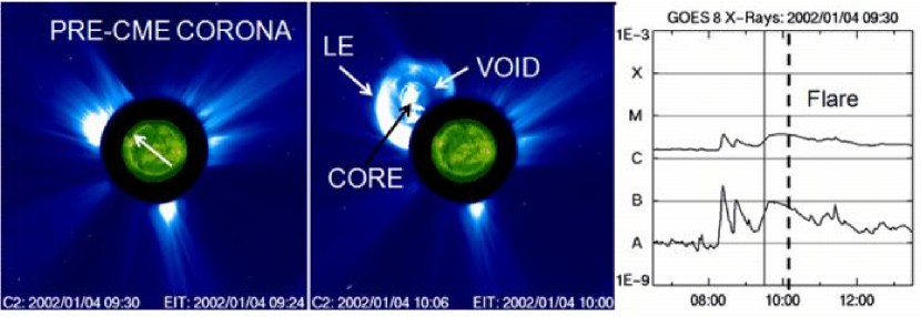
Figure 1: Example of a CME originating from near the northeast limb of the Sun (pointed by arrow) as a distinct structure into the pre-CME corona. The CME roughly fills the northeast quadrant of the Sun. The three primary structures of the CME, viz., the leading edge (LE), which is curved like a loop in 2D projection, the dark void, and the structured prominence core are indicated by arrows. The plot to the right shows the GOES soft X-ray flare associated with the CME. The vertical solid line marks the LASCO frame at 09:30 UT (pre-CME corona) and the dashed line marks the frame with the CME at 10:06 UT.

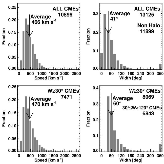
Figure 2: Speed and width distributions of all CMEs (top) and non-narrow CMEs ($W\geq 30^{\circ}$; bottom). The average width of non-narrow CMEs is calculated using only those CMEs with $W\geq 30^{\circ}$.

2 Summary of CME properties

Figure 1 illustrates a CME as a large-scale structure moving in the corona and the associated soft X-ray flare. The CME observations were made by the Solar and Heliospheric Observatory (SOHO) Mission’s Large Angle and Spectrometric Coronagraph (LASCO). The CME is clearly an inhomogeneous structure with a well defined leading edge (LE) followed by a dark void and finally an irregular bright core. The core is nothing but an eruptive prominence normally observed in H$\alpha$ or microwaves, but here observed in the photospheric light Thomson-scattered by the prominence. Prominence eruptions and flares have been known for a long time before the discovery of CMEs in the early 1970s. Several coronagraphs have operated since then and have accumulated a wealth of information on the properties of CMEs (see, e.g., Hundhausen, 1993; Gopalswamy 2004; Kahler, 2006). Here we summarize the statistical properties of CMEs detected by SOHO/LASCO and compiled in a catalog (Gopalswamy et al., 2009c):

• The CME speed is obtained by tracking the leading edge until it reaches the edge of the LASCO field of view (FOV, extending to about 32 R_⊙). Some CMEs become faint before reaching the edge of the FOV and others farther. Therefore, the CME speed we quote here is an average value within the LASCO FOV. Since the height-time measurements are made in the sky plane, the speed is a lower limit. Figure 2 shows that the speed varies over two orders of magnitude from 20 km/s to more than 3000 km/s, with an average value of 466 km/s.

• The CME angular width is measured as the position angle extent of the CME in the sky plane. Figure 2 shows the width distribution for all CMEs and for CMEs with width $>$30^∘. The narrow CMEs ($W<30^{\circ}$) were excluded because the manual detection of such CMEs is highly subjective (Yashiro et al., 2008b). The apparent width ranges from $<$5^∘ to 360^∘ with an average value of 41^∘ (60^∘ when CMEs wider than 30^∘ are considered). There is actually a correlation between CME speed ($V$ km/s) and width ($W$ in degrees) indicating that faster CMEs are generally wider: $V=360+3.64\,W$ (Gopalswamy et al., 2009a).

• CMEs with the above-average speeds decelerate due to coronal drag, while those with speeds well below the average accelerate. CMEs with speeds close to the average speed do not have observable acceleration.

• The CME mass ranges from 10¹² g to $>$10¹⁶ g with an average value of 10¹⁴ g. Wider CMEs generally have a greater mass content ($M$): $\log M=12.6+1.3\log W$ (Gopalswamy et al. 2005). From the observed mass and speed, one can see that the kinetic energy ranges from 10²⁷ erg to $>$10³³ erg, with an average value of $5.4\times 10^{29}$ erg.

• The daily CME rate averaged over Carrington rotation periods ranges from $<0.5$ (solar minimum) to $>6$ (solar maximum). The average speed increases from about 250 km/s during solar minimum to $>550$ km/s during solar maximum (see Fig. 3).

• CMEs moving faster than the coronal magnetosonic speed drive shocks, which accelerate solar energetic particles (SEPs) to GeV energies. The shocks also accelerate electrons, which produce nonthermal radio emission (type II radio bursts) throughout the inner heliosphere.

• The CME eruption is accompanied by solar flares whose intensity in soft X-rays is correlated with the CME kinetic energy (Hundhausen, 1997; Yashiro & Gopalswamy, 2009).

• There is a close temporal and spatial connection between CMEs and flares: CMEs move radially away from the eruption region, except for small deviations that depend on the phase of the solar cycle (Yashiro et al., 2008a). However, more than half of the flares are not associated with CMEs.

• CMEs are comprised of multithermal plasmas containing coronal material at a temperature of a few times $10^{6}$ K and prominence material at about $8000$ K in the core. In-situ observations show high charge states within the CME, confirming the high temperature in the eruption region due to the flare process associated with the CME (Reinard, 2008).

• CMEs originate from closed field regions on the Sun, which are active regions, filament regions, and transequatorial interconnecting regions.

• Some energetic CMEs move as coherent structures in the heliosphere all the way to the edge of the solar system.

• Theory and IP observations suggest that CMEs contain a fundamental flux rope structure identified with the void structure in Fig. 1 (see e.g., Gopalswamy et al., 2006; Amari & Aly, 2009). The prominence core is thought to be located at the bottom of this flux rope. The frontal structure is the material piled up at the leading edge of the flux rope.

• CMEs are often associated with EUV waves, which may be fast mode shocks when the CME is fast enough (Neupert, 1989; Thompson et al., 1998).

• Coronal dimmings are often observed as compact regions located on either side of the photospheric neutral line, which are thought to be the feet of the erupting flux rope (Webb et al. 2000).

Figure 3: The daily CME rate (for CMEs with $W\geq 30^{\circ}$) and the mean CME speed plotted as a function of time showing the solar cycle variation. The occasional spikes are due to super-active regions.

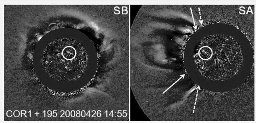
Figure 4: Two images of the 2008 April 26 CME observed simultaneously by the two STEREO spacecraft separated by about $50^{\circ}$. Clearly the CME appears as a halo in the view of the Behind spacecraft (SB), which trailed Earth by about $25^{\circ}$. On the other hand, the CME appears as a normal CME in the view of the Ahead spacecraft (SA) which was ahead of Earth by about $25^{\circ}$. In the SA view, the CME is confined to the angular extent bounded by the two solid arrows. The dashed arrows indicate the disturbances surrounding the CME, which are likely to be shocks for fast CMEs. In the SB view, it is difficult to see the inner and outer structures, so what is seen is likely to be the disturbances surrounding the CME. The solar source of the CME is shown encircled in the difference image taken by STEREO’s Extreme Ultraviolet Imager (EUVI). The elongated feature is the post eruption arcade, which is normally taken as the solar source of the CME. The halo CME is roughly symmetric around the solar source in SB view, while the CME is mostly to the east in the SA view. Thus a top view produces a halo CME, while a broadside view produces a normal CME. Occasionally, the CME can become a halo even in the broadside view; such CMEs are known as “limb halos” because the disturbances can be seen on the limb opposite to the solar source. Such limb halos are generally the fastest events.

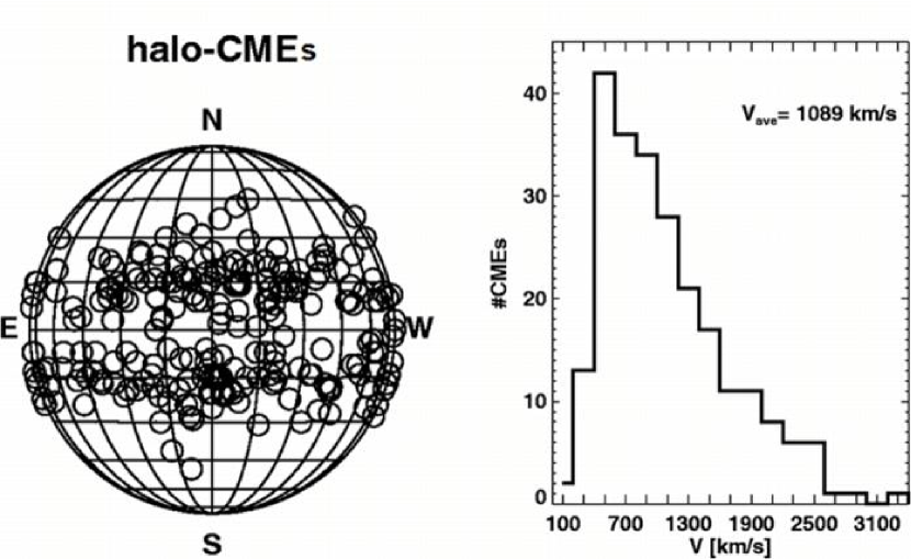
Figure 5: Source locations (left) and the speed distribution (right) of halo CMEs recorded by SOHO during 1996-2007. Note the heavy concentration of the sources close to the central meridian. The average speed of halos ($V_{ave}$) is more than two times the average speed of the general population.

3 Special population of CMEs

In this section, we consider several subsets of CMEs that have significant consequences in the heliosphere: halo CMEs, SEP-producing CMEs, CMEs associated with IP type II radio bursts, CMEs associated with shocks detected in situ, CMEs detected at 1 AU as magnetic clouds and non-cloud ICMEs.

3.1 Halo CMEs

CMEs appearing to surround the occulting disk in coronagraphic images are known as halo CMEs (Howard et al., 1982). Halo CMEs are like any other CMEs except that they move predominantly toward or away from the observer. Figure 4 illustrates this geometrical effect: the same CME is observed from two viewpoints by the Solar Terrestrial Relations Observatory (STEREO) coronagraphs separated by an angle of $50^{\circ}$. In the SOHO data $3.6$% of all CMEs were found to be full halos, while CMEs with $W\geq 120^{\circ}$ account for $11$% (Gopalswamy, 2004). Coronagraph occulting disks block the solar disk and the inner corona, so observations in other wavelengths such as H$\alpha$, microwave, X-ray or EUV are needed to determine whether a CME is frontsided or not. Fig. 5 shows the source locations of halo CMEs defined as the heliographic coordinates of the associated flares. Clearly, most of the sources are concentrated near the central meridian. Halos within a central meridian distance (CMD) of $45^{\circ}$ are known as disk halos, while those with $45^{\circ}<\rm{CMD}\leq 90^{\circ}$ are known as limb halos. Halos occurring close to the central meridian appear as symmetric halos in the coronagraph images. Halos originating from close to the limb appear asymmetric (see Gopalswamy et al., 2003a). The outermost structures seen in most of the halos are likely to be the disturbances (shocks) surrounding the main body of the CME (Sheeley et al., 2000). When the halo CMEs erupt on the visible face of the Sun, they are highly likely to impact Earth and cause intense geomagnetic storms. About 70% of the halos have been found to be geoeffective ($Dst\leq-50$ nT). Disk halos are more geoeffective by their direct impact on Earth, while the limb halos are less geoeffective because of the glancing impact they deliver. More details on halo CMEs can be found in Gopalswamy et al. (2007).

The speed distribution in Fig. 5 shows that the halos are high-speed CMEs (the average speed is about 1090 km/s, more than two times the average speed of all CMEs). The halo CMEs are also associated with flares of greater X-ray importance (Gopalswamy et al., 2007). Halo CMEs observed from a single spacecraft have no width information. However, higher-speed CMEs have been found to be wider from a set of CMEs erupting close to the limb (Gopalswamy et al., 2009a). Furthermore, wider CMEs are more massive (Gopalswamy et al., 2005). Therefore, one can conclude that halos are more energetic on the average. This is the reason that a large fraction of halos are important for space weather as they drive shocks that produce SEPs and produce geomagnetic storms.

3.2 CMEs resulting in ICMEs

CMEs in the IP medium are known as IP CMEs or ICMEs for short. ICMEs are generally inferred from single point observations from the solar wind plasma, magnetic field and composition signatures as the ICME blows past the observing spacecraft (see Gosling, 1996 for a discussion on the identification of ICMEs). ICMEs can be traced back to the frontside of the Sun by looking at 5 days of solar observations preceding the ICME arrival at Earth. When ICMEs have a flux rope structure with depressed proton temperature compared to the pre-ICME solar wind, they are known as magnetic clouds (MCs) or IP flux ropes (Burlaga et al., 1981). CMEs resulting in MCs generally originate close to the disk center. CMEs resulting in non-cloud ICMEs generally originate at CMD $>30^{\circ}$, but there are many exceptions. Shock-driving ICMEs are easier to identify because shocks are well-defined discontinuities observed in the solar wind. Sometimes, IP shocks are observed without a discernible ICME. In these cases the CMEs are ejected at large angles to the Sun-Earth line, so the ICME part misses Earth. Thus as one goes from the disk center to the limb, one encounters solar sources of MCs close to the disk center, those of non-clouds ICMEs, and finally shocks without drivers (Gopalswamy, 2006). This suggests the IP manifestation of CMEs depends on the observer–Sun–CME angle. Assuming that CMEs reaching 1 AU have an average width of $60^{\circ}$, one can see that about one third of such CMEs should be MCs and the remaining two-thirds should be non-cloud ICMEs (excluding the pure shock cases). This is generally the case on the average (e.g., Burlaga, 1995), but there are notable exceptions: (i) the fraction of MCs is very high during the rise phase of the solar cycle compared to the maximum phase (Riley et al., 2006), (ii) there are many non-cloud ICME sources close to the disk center, (iii) some pure-shock sources are close to the disk center during the declining phase. These exceptions can be explained as the effect of external influences (Gopalswamy et al., 2009b).

ICMEs reaching Earth are highly likely to cause magnetic storms, provided they contain south-pointing magnetic field either in the ICME portion or in the sheath portion or both. In fact about 90% of the large geomagnetic storms are due to ICME impact on Earth’s magnetosphere. The remaining 10% of the large storms are caused by corotating interaction regions (CIRs) resulting from the interaction between fast and slow solar wind streams (see e.g., Zhang et al., 2007).

3.3 Shock-driving CMEs

CMEs driving fast mode MHD shocks can be directly observed in the solar wind. Occurrence of type II radio bursts at the local plasma frequency in the vicinity of the observing spacecraft (Bale et al., 1999) is strong evidence that the radio bursts are produced by electrons accelerated at the shock front by the plasma emission mechanism first proposed by Ginzburg and Zhelezniakov (1958). The frequency of type II burst emission is related to the plasma density in the corona, so high frequency (about 150 MHz) type II bursts are indicative of shocks accelerating electrons near the Sun. CMEs must have speeds exceeding the local fast-mode speed in order to drive a shock. CMEs associated with metric type II bursts have a speed of about 600 km/s, while those producing type II bursts at decameter-hectometric (DH) wavelengths have an average speed exceeding 1100 km/s. Type II bursts with emission components from metric to kilometric wavelengths are associated with the fastest CMEs (average speed about $1500$ km/s). Thus type II bursts are good indicators of shock-driving CMEs (Gopalswamy et al., 2005). Here we take type II bursts at DH wavelengths to be indicative of CMEs driving IP shocks. However, not all DH type II bursts are indicative of shocks detected in situ. This is mainly because CMEs originating even behind the limbs can produce type II bursts because of the extended nature of the shock and the wide beams of the radio emission, but these shocks need not reach Earth. On the other hand, there are some shocks detected at 1 AU, which are not associated with DH type II bursts; shocks have to be of certain threshold strength to accelerate electrons.

A subset of shock-driving CMEs are associated with solar energetic particle (SEP) events detected near Earth. Naturally, the associated CMEs form a subset of those producing DH type II bursts because the same shocks accelerate electrons and ions. In fact, all the major SEP events are associated with DH type II bursts (Gopalswamy, 2003; Cliver et al., 2004), but only about half of the DH type II bursts have SEP association (Gopalswamy et al., 2008). CMEs associated with SEP events have the highest average speed (about 1600 km/s).

Table 1: Speed and width of the special populations of CMEs

	Halos	MCs	Non-MCs	Type IIs	Shocks	Storms	SEPs
Speed (km/s)	1089	782	955	1194	966	1007	1557
% Halos	100	59	60	59	54	67	69
% Partial Halos	–	88	90	81	90	91	88
Non-halo Width (∘)	–	55	84	83	90	89	48

3.4 Comparing the properties of the special populations

Table 1 compares the speed and width information of the special population of CMEs discussed above. The lowest average speed is for MC-associated CMEs and the highest speed is for SEP-producing CMEs. The cumulative speed distribution of all CMEs is shown in Fig. 6 with the lowest and highest speeds in Table 1 marked. Even the lowest speed (782 km/s for MCs) in Table 1 is well above the average speed of all CMEs. The average speed of the SEP-producing CMEs is the highest (1557 km/s). All the other special populations have their average speeds between these two limits.

The fraction of halo CMEs in a given population is an indicator of the energy of the CMEs, because halo CMEs are more energetic on the average owing to their higher speed and larger width. The majority of CMEs in all special populations are halos. If partial halos are included, the fraction becomes more than 80% in each population. Even the small fraction of non-halo CMEs ($W<120^{\circ}$) have an above-average width. The large fraction of halos in each population implies that there is a high degree of overlap among the populations, i.e., the same CME appears in various subgroups.

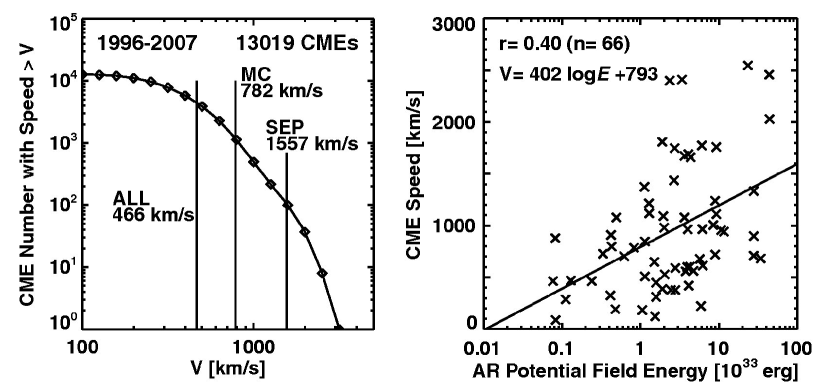
Figure 6: Left: the cumulative number distribution of CMEs as a function of speed ($V$). The average speed of all CMEs (466 km/s), CMEs resulting in MCs (782 km/s), and CMEs producing SEPs (1557 km/s) are indicated. Note that the number of CMEs with speeds $>$3000 km/s is negligibly small. Right: scatter plot between active-region (AR) potential energy ($E$) and $V$ for a set of 66 CMEs that had significant impact on Earth. These CMEs either produced large geomagnetic storms or became MCs. E was calculated using the AR flux ($\phi$) and area $A$ measured when the AR was close to the central meridian (CMD $\leq$45^∘) as follows: $E=\phi^{2}/8\pi\sqrt{A}$. The scatter plot shows a weak correlation ($r=0.40$). The regression line is also shown on the plot.

From Fig. 6 one can see that the number of CMEs with speeds $>$ 2000 km/s is exceedingly small. In fact, only two CMEs are known to have speeds exceeding 3000 km/s among the more than 13000 CMEs detected by SOHO during 1996 to 2007. This implies a limit to the speed that CMEs can attain of about $4000$ km/s. For a mass of about $10^{17}$ g, a 4000 km/s CME would possess a kinetic energy of $10^{34}$ erg. Active regions that produce such high energy CMEs must possess a free energy of at least $10^{34}$ erg to power the CMEs. It has been estimated that the free energy in active regions is of the order of the potential field energy and that the total magnetic energy in the active region is about twice the potential field energy (Mackay et al., 1997; Metcalf et al., 1995; Forbes, 2000; Venkatakrishnan and Ravindra, 2003). The potential field energy depends on the size and the average magnetic field strength in the active regions. Figure 6 shows a scatter plot between the potential field energy and the CME speed for a set of CMEs that produced large geomagnetic storms or arrived at Earth as MCs. The correlation is weak but there is certainly a trend that faster CMEs arise from regions of higher potential field energy, as previously shown by Venkatakrishnan and Ravindra (2003). The limiting speed of the CMEs can thus be traced to the maximum energy that can be stored in solar active regions. The largest reported active region size is about $5000$ millionths of a solar hemisphere (Newton, 1955), and the highest magnetic field strength observed in sunspots is about 6100 G (Livingston et al., 2006). Combining these two, one can estimate an upper limit of $10^{36}$ erg for the potential field energy and hence the free energy that can be stored in an active region. Usually a single CME does not exhaust all the free energy in the active region. Note that some stars have much larger spots and can release a lot more energy than in solar eruptions (Byrne, 1988).

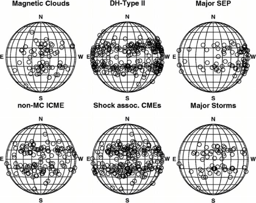
Figure 7: Heliographic coordinates of the solar sources of the special populations.

3.5 Solar sources of the special populations

The lowest speed of the MC-associated CMEs and the highest speed of the SEP-associated CMEs shown in Table 1 may be partly due to projection effects because the speeds were measured in the sky plane. To see this, we have shown the distributions of the solar sources of the special populations in Fig. 7. The solar sources are taken as the heliographic coordinates of the associated H$\alpha$ flares from the Solar Geophysical Data. For events with no reported flare information, we have taken the centroid of the post eruption arcade from EUV, X-ray or microwave images as the solar source. CMEs associated with MCs generally originate from the disk center, so they are subject to projection effects; the SEP-associated CMEs are mostly near the limb, so the projection effects are expected to be minimal. Note that the speed difference between MC- and SEP-associated CMEs is similar to that of disk and limb halo CMEs (933 km/s vs. 1548 km/s – see Gopalswamy et al., 2007). It is also possible that the SEP associated CMEs are the fastest because they have to drive shocks and accelerate particles.

The solar source distributions in Fig. 7 reveal several interesting facts: (i) Most of the sources are at low latitudes with only a few exceptions during the rise phase. (ii) The MC sources are generally confined to the disk center, but the non-cloud ICME sources are distributed at larger CMD. There is some concentration of the non-MC sources to the east of the central meridian. (iii) Subsets of MCs and non-MC ICMEs are responsible for the major geomagnetic storms, so the solar sources of storm-associated CMEs are also generally close to the central meridian. The slight higher longitudinal extent compared to that of MC sources is due to the fact that some storms are produced by shock sheaths of some fast CMEs originating at larger CMD. (iv) The solar sources of CMEs producing DH type II bursts have nearly uniform distribution in longitude, including the east and west limbs. There are also sources behind the east and west limbs that are not plotted. The radio emission can reach the observer from large angles owing to the wide beam of the radio bursts. (v) The sources of SEP-associated CMEs, on the other hand, are confined mostly to the western hemisphere with a large number of sources close to the limb. In fact there are also many sources behind the west limb, not plotted here (see Gopalswamy et al., 2008a for more details). This western bias is known to be due to the spiral structure of the IP magnetic field along which the SEPs have to propagate before being detected by an observer near Earth. Typically the longitude W70 is well connected to an Earth observer. An observer located to the east is expected to detect more particle events from the CMEs that produce DH type II bursts but located on the eastern hemisphere. There are a few eastern sources producing SEPs, but these are generally low-intensity events from very fast CMEs. (vi) The shock sources are quite similar to the DH type II sources except for the limb part. Since the associated CMEs need to produce a shock signature at Earth, they are somewhat restricted to the disk. Occasional limb CMEs did produce shock signatures at Earth, but these are shock flanks. Comparison with DH type II sources reveals that many shocks do not produce radio emission probably due to the low Mach number (Gopalswamy et al., 2008b).

It is also interesting to note that the combined MC and non-cloud ICME source distribution is similar to those of halo CMEs and the ones associated with shocks at 1 AU. Even the sources of the SEP associated CMEs are similar to the halos originating from the western hemisphere of the Sun because of the requirement of magnetic connectivity to the particle detector.

Figure 8: The source latitudes of the special populations plotted as a function of time: halo CMEs, CMEs detected in situ as ICMEs, CMEs producing DH type II bursts, CMEs driving IP shocks, CMEs producing large SEP events, and CMEs resulting in large geomagnetic storms ($Dst\leq-100$ nT). The solid vertical line (end of the year 1998) divides the rise and maximum phases. The dashed vertical line (end of May 2002) divides the maximum and declining phases. This line also marks the end of polarity reversal at solar poles (i.e., beginning of the new solar magnetic cycle). CMEs from the three phases of solar cycle 23 are also distinguished by different symbols (rise - open circles, maximum - triangles, and declining - squares).

4 Solar cycle variation

CMEs originating close to the disk center and in the western hemisphere have important implications to the space environment of Earth because of the geomagnetic storms and the SEP events they produce. Source regions of CMEs come close to the disk center in two ways: (i) the solar rotation brings active regions to the central meridian, and (ii) the progressive decrease in the latitudes where active regions emerge from beneath the photosphere (the butterfly diagram). The effect due to the solar rotation is of short-term because an active region stays in the vicinity of the disk center only for 3–4 days during its disk passage. In order to see the effect of the butterfly diagram, we need to plot the solar sources of as a function of time.

Figure 8 shows the latitude distribution of the solar sources of the special populations as a function of time during solar cycle 23. Sources corresponding to the three phases of the solar cycle are distinguished using different symbols: the rise phase starts from the beginning of the cycle in 1996 to the end of 1998. The maximum phase is taken from the beginning of 1999 to the middle of 2002. The time of completion of the polarity reversal of the solar polar magnetic fields is considered as the end of the solar maximum phase and the beginning of the declining phase. The boundary between phases is not precise, but one can see the difference in the levels of activity and the change in latitude between phases. We have combined the MCs and non-MC ICMEs into a single group as ICMEs. As we noted before, there is a close similarity between the ICME and halo CME sources because many frontside halo CMEs become ICMEs (see the left column in Fig. 8. There are clearly ICMEs without corresponding halos, which means some ICMEs are due to non-halo CMEs. During the rise phase there are several sources at latitudes higher than the ones at which sunspots emerge (about $40^{\circ}$). What is striking is that such high-latitude CMEs produced an observable signature at Earth. Case studies (Gopalswamy et al., 2000, Gopalswamy & Thompson, 2000) and statistical studies (Plunkett et al., 2001; Gopalswamy et al., 2003b; Cremades et al., 2006) have shown that CMEs during the solar minimum get deflected towards the equator because of the strong global dipolar field of the Sun. In the declining phase, a different type of deflection occurs: eruptions occurring near low latitude coronal holes tend to be deflected away from coronal holes. Occasionally, such deflections push CMEs toward or away from the Sun-Earth line (Gopalswamy et al., 2009c).

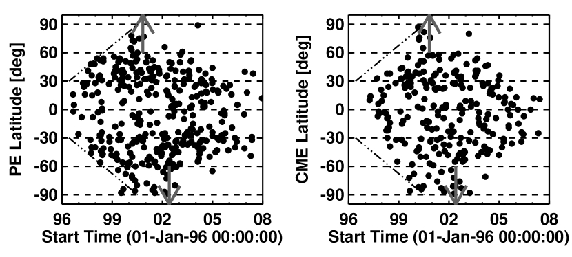
Figure 9: Latitude of prominence eruptions (PEs) and those of the associated CMEs shown as a function of time. The up and down arrows denote respectively the times when the polarity in the north and south solar poles reversed. Note that the high-latitude CMEs and PEs are confined to the solar maximum phase and their occurrence is asymmetric in the northern and southern hemispheres. PEs at latitudes below 40^∘ may be from active regions or quiescent filament regions, but those at higher latitudes are always from the latter.

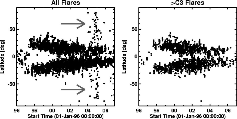
Figure 10: Flare locations reported in the Solar Geophysical Data plotted as a function of time for all flares (left) and larger flares (soft X-ray importance $>$C3.0) (right). The arrows point to the weak flares from higher latitudes. Note that the GOES Soft X-ray imager provided solar source locations of flares only during January 2004 to March 2007, so there is no information on the high-latitude flare locations for other times.

Despite the longitudinal differences presented in Fig. 8, we see a close latitudinal similarity of the solar sources of the special populations. The sources clearly follow the sunspot butterfly diagram. This means the special populations originate only from active regions, where one expects to have higher free energy needed to power these energetic CMEs.

4.1 Solar sources of the general population

In contrast to the solar sources of the special populations discussed above, the general CME population is known to occur at all latitudes during solar maxima (Hundhausen, 1993; Gopalswamy et al., 2003b). Figure 9 illustrates this using the latitude distributions of prominence eruptions (PEs) and the associated CMEs. Note that these CMEs constitute a very small sample because they are chosen based on their association with PEs detected by the Nobeyama radioheliograph (Nakajima et al., 1994), which is a ground based instrument operating only about $8$ h per day. Nevertheless, the observations provide accurate source information for the CMEs and the sample is not subject to projection effects. One can clearly see a large number of high latitude CMEs between the years 1999 and 2003, with a significant north-south asymmetry in the source distributions. These high-latitude CMEs are associated with polar crown filaments, which migrate toward the solar poles and completely disappear by the end of the solar maximum. The cessation of high-latitude CME activity has been found to be a good indicator of the polarity reversal at solar poles (Gopalswamy et al., 2003c). Low-latitude PEs may be associated with both active regions and quiescent filament regions, but the high-latitude CMEs are always associated with filament regions. One can clearly see that the high-latitude CMEs have no relation to the sunspot activity because the latter is confined to latitudes below $40^{\circ}$. Comparing Figures 8 and 9 we can conclude that the special populations are primarily an active region phenomenon. It is interesting that the high-latitude CMEs occur only during the period of maximum sunspot number (SSN), but are not directly related to the sunspots.

4.2 Implications to the flare – CME connection

The difference in the latitude distributions of CMEs (no butterfly diagram) and flares (follow the sunspot butterfly diagram) coupled with the weak correlation between CME kinetic energy and soft X-ray flare size (Hundhausen, 1997) has been suggested as evidence that CMEs are not directly related to flares. However, this depends on the definition of flares. If flares are defined as the enhanced electromagnetic emission from the structures left behind after CME eruptions, one can find flares associated with all CMEs – both at high and at low latitudes. This is illustrated using Fig. 10, which shows the solar source locations of flares reported in the Solar Geophysical Data. During 2004 January - 2007 March, the GOES Soft X-ray Imager (SXI) provided the solar sources of all flares, including the weak ones that can be found at all latitudes, similar to the source distribution shown in Fig. 9 for PEs. On the other hand if we consider only larger flares (X-ray importance $>$C3.0), we see that the flares follow the sunspot butterfly diagram. This is quite consistent with the fact that the solar sources of the special populations of CMEs follow the sunspot butterfly diagram because these CMEs are associated with larger flares. For example, the median size of flares associated with halo CMEs is M2.5, an order of magnitude larger than the median size of all flares (C1.7) during solar cycle 23 (Gopalswamy et al., 2007). Thus, CMEs seem to be related to flares irrespective of the origin in active regions or quiescent filament regions. There are in fact several new indicators of the close connection between CMEs and flares: CME speed and flare profiles (Zhang et al., 2001), CME and flare angular widths (Moore et al., 2007), CME magnetic flux in the IP medium and the reconnection flux at the Sun (Qiu et al., 2007), and the CME and flare positional correspondence (Yashiro et al., 2008a). The close relationship between flares and CMEs does not contradict the fact that more than half of the flares are not associated with CMEs. This is because the stored energy in the solar source regions can be released to heat the flaring loops with no mass motion.

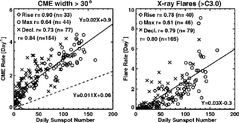
Figure 11: Correlation of the daily sunspot number with the daily CME rate (left) and the daily flare rate (right). All numbers are averaged over Carrington rotation periods (27.3 days). The number of rotations (n) is different for the CME and flare rates because of CME data gaps. Rates in different phases of the solar cycle are shown by different symbols. The correlation coefficients are also shown for individual phases as well as for the entire data set (the solid lines are the regression lines). In the CME rate, only CMEs wider than 30^∘ are used to avoid subjectivity in CME identification. In the CME plot, the dashed line corresponds to the regression line (Y = 0.011X + 0.06) obtained by Cliver et al. (1994) for CMEs from the pre-SOHO era. In the flare rate, only flares of importance $>$C3.0 are included.

5 Sunspot number and CME rate

The above discussion made it clear that the high-latitude CMEs do not follow the sunspot butterfly diagram but occur during the period of maximum solar activity. This should somehow be reflected in the relation between CME and sunspot activities. To see this, we have plotted the daily CME rate ($R$) as a function of the daily sunspot number (SSN) in Fig. 11. There is an overall good correlation between the two types of activity, which has been known for a long time (Hildner et al., 1976; Webb et al. 1994; Cliver et al., 1994; Gopalswamy et al., 2003a). The SOHO data yield a relation $R=0.02\,\rm{SSN}+0.9$ (correlation coefficient $r=0.84$), which has a larger slope compared to the one obtained by Cliver et al. (1994): $R=0.011\,\rm{SSN}+0.06$. The higher rate has been attributed to the better dynamic range and wider field of view of the SOHO coronagraphs compared to the pre-SOHO coronagraphs. However, when the CMEs are grouped according to the phase of the solar cycle, the correlation becomes weak during the maximum phase ($r=0.64$) compared to the rise ($r=0.90$) and declining ($r=0.73$) phases. We attribute this diminished correlation to the CMEs during the maximum phase that are not associated with sunspots (see also Gopalswamy et al., 2003a). Note that we have excluded narrow CMEs ($W<30^{\circ}$) because manual detection of such CMEs is highly subjective.

A similar scatter plot involving the daily flare rate as a function of SSN reveals a similar trend in terms of the overall correlations ($r=0.80$) and the individual phases: rise ($r=0.78$), maximum ($r=0.61$) and declining ($r=0.79$). In particular, the weak correlation between the flare rate and SSN during the maximum phase is striking. When all the flares are included, the overall correlation diminished only slightly ($r=0.76$) mainly due to the weaker correlation during the maximum phase ($r=0.46$) because the correlation remained high during the rise ($r=0.85$), and declining ($r=0.79$) phases. Interestingly, flare rate vs. SSN correlations are very similar to the CME rate vs. SSN correlations, including the weaker correlation during the maximum phase. This needs further investigation by separating the flares into high and low-latitude events.

6 Summary and conclusions

In this paper, we studied several subsets of CMEs that have significant consequences in the heliosphere: halo CMEs, SEP-producing CMEs, CMEs associated with IP type II radio bursts, CMEs associated with shocks detected in situ in the solar wind, CMEs detected at 1 AU as magnetic clouds and non-cloud ICMEs. The primary common property of these special populations is their above-average energy, which helps them propagate far into the IP medium. Most of the CMEs in these subsets are frontside halo CMEs. Notable exceptions are the IP type II bursts and large SEP events. IP type II bursts can be observed from CMEs from behind the east and west limbs because the shocks responsible for the radio emission are more extended than the driving CMEs, and the radio emission is wide beamed. SEP events are also observed from behind the west limb for the same reason (extended shock) and the fact that the SEPs propagate from the shock to the observer along the spiral magnetic field lines. Another common property of the special populations is that they follow the sunspot butterfly diagram. This suggests that the energetic CMEs originate mostly from the sunspot regions, where large free energy can be stored to power the energetic CMEs. Quiescent filament regions are the other source of CMEs, not related to the sunspots, and hence do not follow the sunspot butterfly diagram. During the maximum phase of the solar activity cycle, the quiescent filament regions occur in high abundance at high latitudes, resulting in higher rate of CMEs from there. Since the high-latitude CMEs are not related to the sunspots, the correlation between daily CME rate and sunspot number is weak in the maximum phase. A similar weak correlation was found between the flaring rate and sunspot number during the maximum phase. This result further confirms the close relation between flares and CMEs irrespective of the source region: sunspot regions or quiescent filament regions.