High-energy gluon bremsstrahlung in a finite medium: harmonic oscillator versus single scattering approximation

Abstract

A particle produced in a hard collision can lose energy through bremsstrahlung. It has long been of interest to calculate the effect on bremsstrahlung if the particle is produced inside a finite-size QCD medium such as a quark-gluon plasma. For the case of very high-energy particles traveling through the background of a weakly-coupled quark-gluon plasma, it is known how to reduce this problem to an equivalent problem in non-relativistic two-dimensional quantum mechanics. Analytic solutions, however, have always resorted to further approximations. One is a harmonic oscillator approximation to the corresponding quantum mechanics problem, which is appropriate for sufficiently thick media. Another is to formally treat the particle as having only a single significant scattering from the plasma (known as the $N{=}1$ term of the opacity expansion), which is appropriate for sufficiently thin media. In a broad range of intermediate cases, these two very different approximations give surprisingly similar but slightly differing results if one works to leading logarithmic order in the particle energy, and there has been confusion about the range of validity of each approximation. In this paper, I sort out in detail the parametric range of validity of these two approximations at leading logarithmic order. For simplicity, I study the problem for small $\alpha_{\rm s}$ and large logarithms but $\alpha_{\rm s}\log\ll 1$.

I Introduction and Results

I.1 Background

There is a prototypical toy problem often considered in theoretical discussions of gluon bremsstrahlung in a QCD medium such as a quark-gluon plasma: Consider a high-energy quark or gluon that is produced by some hard scattering event and then propagates through a length $L$ of a uniform QCD medium before emerging into vacuum. What is the effect of the medium on the probability for gluon bremsstrahlung from this high-energy particle? This is known as the brick problem. The problem is complicated by the Landau-Pomeranchuk-Migdal (LPM) effect LP ; Migdal . The quantum mechanical duration (formation time) of the bremsstrahlung process grows with increasing energy and eventually exceeds the mean free time between collisions. As a result, successive collisions of the high-energy particle with the plasma cannot be treated as independent from each other for the purpose of calculating the probability of bremsstrahlung.

There is a general formalism for treating this problem, but analytic solutions have required additional approximations. Baier, Dokshitzer, Mueller, and Schiff (BDMS) BDMS investigated the problem in the limit that the energy was high enough, and the medium thick enough, that the number of collisions $N$ within the bremsstrahlung formation time was large — so large that $\ln N$ could be treated as large. In this limit, they made an approximation, known as the harmonic oscillator (HO) approximation, that reduced the general formalism to a certain type of harmonic oscillator problem. They solved for the medium effects on the spectrum of gluon bremsstrahlung, to be reviewed below. From the spectrum, they computed the size $\Delta E$ of the medium effect on the average energy loss of a high-energy particle of energy $E$. The qualitative form of their result depends on the thickness $L$ of the medium compared to the typical formation length $L_{\infty}$ for gluon bremsstrahlung in an infinite medium, which is parametrically

$$L_{\infty}\sim\sqrt{\frac{E}{\hat{q}}}.$$ (1)

Here, $\hat{q}$ is the typical squared transverse momentum per unit length transferred via elastic collisions to a high-energy particle as it traverses the medium (more discussion later). For thick media ($L\gg L_{\infty}$), they found that $\Delta E$ grows linearly with $L$, as one would expect. For thin media ($L\ll L_{\infty}$), they found BDMS

$$\Delta E_{\rm HO}\simeq\tfrac{1}{4}C_{s}\alpha\hat{q}_{\rm A}L^{2}\simeq\pi C_{s}C_{\rm A}\alpha^{3}{\cal N}L^{2}\ln\left(\frac{\hat{q}_{\rm A}L}{m_{\rm D}^{2}}\right),$$ (2)

to leading order in inverse powers of the logarithm. Here $s$ is the species (quark or gluon) of the high-energy particle, and $C_{R}$ is the quadratic Casimir of a given color representation. ${\cal N}$ is the density $n$ of plasma particles weighted by group factors as

$${\cal N}=\frac{1}{d_{\rm A}}\left[C_{\rm A}n_{\rm g}+C_{\rm F}(n_{\rm q}+n_{\rm\bar{q}})\right]=\tfrac{3}{8}\,n_{\rm g}+\tfrac{1}{6}(n_{\rm q}+n_{\rm\bar{q}})=\frac{6\,\zeta(3)}{\pi^{2}}\Bigl{(}1+\tfrac{1}{4}N_{\rm f}\Bigr{)}T^{2},$$ (3)

where $N_{\rm f}$ is the number of quark flavors.

In contrast, various other authors have investigated the opposite approximation, starting from early work by Wiedemann and Gyulassy WiedemannGyulassy and by Gyulassy, Levai, and Vitev (GLV) GLV ; GLV2a ; GLV2b . Instead of treating the number $N$ of elastic collisions as large, they expand order by order in the number of collisions. This is known as the opacity expansion. The leading term, corresponding to $N=1$, gives

$$\Delta E_{N{=}1}\simeq\pi C_{s}C_{\rm A}\alpha^{3}{\cal N}L^{2}\ln\left(\frac{E}{m_{\rm D}^{2}L}\right)$$ (4)

in the high-energy limit, to leading order in inverse powers of $\ln(E/m_{\rm D}^{2}L)$.

The results (2) and (4) from opposite assumptions about the relevant number of collisions are surprisingly similar, differing only in the argument of the logarithm. Two natural questions arise. Which formula is correct for what range of media thickness $L$? Which description captures the correct physics: Is there a single collision with the medium which dominates the medium’s contribution to bremsstrahlung energy loss, or is $\Delta E$ dominated by processes where many scatterings are important?

The qualitative difference between the HO and $N{=}1$ approximations becomes more pronounced if one looks more generally at the gluon bremsstrahlung spectrum instead of focusing on the single number $\Delta E$. For the brick problem, the HO approximation gives the result BDMS

$$\omega\,\frac{d}{d\omega}(I-I_{\rm vac})_{\rm HO}=\frac{\alpha}{\pi}\,x\,P_{s{\to}{\rm g}}(x)\,\ln\left|\cos(\omega_{0}L)\right|$$ (5)

with

$$\omega_{0}^{2}=-i\,\frac{[(1-x)\hat{q}_{\rm A}+x^{2}\hat{q}_{s}]}{2x(1-x)E}\,.$$ (6)

Here, $I$ is the probability of gluon bremsstrahlung, with $I_{\rm vac}$ the corresponding probability if the process which created the high-energy particle had instead taken place in vacuum. $P_{s\to g}(x)$ is the usual vacuum splitting function, $\omega$ is the energy of the (high-energy) bremsstrahlung gluon, and $x\equiv\omega/E$ is its momentum fraction. $|\omega_{0}|^{-1}$ is of order the formation length $l_{\infty}(\omega)$ for a bremsstrahlung gluon of frequency $\omega$ in an infinite medium. The previous formula (2) for $\Delta E$ is just the $\omega$ integral of (5) in the limit $L\ll L_{\infty}$. In that limit, the $\omega$ integral is dominated by small $x$ such that $l_{\infty}(\omega)\sim L$. But now fix $\omega$ and consider thinner and thinner media such that $L$ is small compared to the formation length $l_{\infty}(\omega)$. The small $L$ limit of (5) is

$$\omega\,\frac{d}{d\omega}(I-I_{\rm vac})_{\rm HO}\simeq\frac{\alpha}{\pi}\,x\,P_{s{\to}{\rm g}}(x)\,\frac{|\omega_{0}L|^{4}}{12}$$ (7)

Focusing on the case $x\ll 1$, for simplicity, gives

$$\omega\,\frac{d}{d\omega}(I-I_{\rm vac})_{\rm HO}\simeq\frac{C_{s}\alpha\hat{q}_{\rm A}^{2}}{24\pi\omega^{2}}\,L^{4}\simeq\frac{2\pi C_{s}C_{\rm A}^{2}\alpha^{5}{\cal N}^{2}}{3\omega^{2}}\,L^{4}\ln^{2}\left(\frac{\hat{q}_{\rm A}L}{m_{\rm D}^{2}}\right),$$ (8)

where the last equality relies on the formula for $\hat{q}$, to be reviewed momentarily. In contrast, the $N{=}1$ term of the opacity expansion gives

$$\omega\,\frac{d}{d\omega}(I-I_{\rm vac})_{N{=}1}\simeq\frac{\pi C_{s}C_{\rm A}\alpha^{3}{\cal N}}{\omega}\,L^{2}.$$ (9)

Because it is proportional to $L^{2}$ rather than $L^{4}$, the $N{=}1$ result clearly dominates over the HO result for small $L$. The HO result seems completely at odds with the $N{=}1$ result for small $L$. When is the HO result correct?

All of these issues were raised some years ago by Zakharov ZakharovResolution . He concluded that the HO analysis should not be trusted in cases when the medium thickness $L$ is less than or order the relevant formation length $L_{\infty}$ or $l_{\infty}(\omega)$. In this paper, I return to this problem and show that the HO approximation is valid over a wider range of $L$, and I elucidate in more detail the interplay between contributions to bremsstrahlung (i) arising from large numbers of scatterings and (ii) dominated by a single scattering.

I will assume that the particle energy $E$ is so large that $\ln(E/T)$ can be treated as a large number, where $T$ is the plasma temperature. Because I want to pursue a qualitative understanding of how the HO and $N{=}1$ results fit together, I will usually just focus on the parametric form of formulas. Though I will treat logarithms as large, I will formally assume that $\alpha$ is so small that $\alpha\ln(E/T)$ is small. So, for instance, I will ignore running of the coupling and treat $\alpha$ as fixed. The purpose of these various limits is to provide a clean, theoretical situation for conceptually disentangling the HO and $N{=}1$ approximations. For experimentally achievable quark-gluon plasmas, of course, logarithms are not huge and $\alpha$ is not tiny.

I.2 Transverse momentum diffusion

To describe my results, it is useful to first characterize the total transverse momentum $Q_{\perp}$ that a high-energy particle picks up, due to screened Coulomb-like interactions, as it crosses length $L$ of a QCD medium. In a perturbative quark-gluon plasma, the differential elastic scattering rate for a high-energy particle to pick up transverse momentum $q_{\perp}$ is

$$\frac{d\Gamma_{\rm el}}{d^{2}q_{\perp}}\simeq\frac{4C_{R}\alpha^{2}{\cal N}}{q_{\perp}^{4}}\,,$$ (10)

for $q_{\perp}\gg T$. The behavior is similar, with a slightly different coefficient, for smaller $q_{\perp}$ down to $m_{\rm D}$, where Debye screening kicks in. Over multiple collisions, the net transverse momentum transfer will random walk, and its average will be

$$(Q_{\perp}^{2})_{\rm avg}=L\int d^{2}q_{\perp}\frac{d\Gamma_{\rm el}}{d^{2}q_{\perp}}q_{\perp}^{2}.$$ (11)

Using (10), this integral has a well-known logarithmic divergence which is cut off in the infrared by Debye screening. The UV end is cut off by the kinematic limit $q_{\perp}^{\rm max}\sim\sqrt{ET}$, where the plasma temperature $T$ gives the typical energy of a plasma particle. However, the average $Q_{\perp}^{2}$ will not be an interesting quantity for our purposes. The probability that there is at least one collision with individual momentum transfer of order $q_{\perp}$ over the distance $L$ is of order

$$\min\left(q_{\perp}^{2}\frac{d\Gamma_{\rm el}}{d^{2}q_{\perp}}\,L\,,1\right)\sim\min\left(\frac{C_{R}\alpha^{2}{\cal N}L}{q_{\perp}^{2}}\,,1\right)$$ (12)

So it is unlikely to have any individual collisions with $q_{\perp}^{2}\gg C_{R}\alpha^{2}{\cal N}L$. If we are interested in the typical (i.e. median) $Q_{\perp}^{2}$ instead of the average $Q_{\perp}^{2}$, we should use this value of $q_{\perp}^{2}$ as an upper cut-off on the integration in (11). The result is then

$$(Q_{\perp}^{2})_{\rm typ}=\hat{q}_{R}L$$ (13a)

with

$$\hat{q}_{R}\simeq 4\pi C_{R}\alpha^{2}{\cal N}\ln\left(\frac{C_{R}\alpha^{2}{\cal N}L}{m_{\rm D}^{2}}\right)$$ (13b)

for a particle with color representation $R$. Throughout this paper, I will use $\hat{q}$ to denote the typical (rather than average) squared transverse momentum acquired per unit length, as given by (13b).

A simple way that one can get to an equivalent result is to self-consistently use $Q_{\perp}$ itself to cut off the UV logarithmic divergence in (11), so that

$$(Q_{\perp}^{2})_{\rm typ}\simeq 4\pi C_{R}\alpha^{2}{\cal N}L\ln\left(\frac{(Q_{\perp}^{2})_{\rm typ}}{m_{\rm D}^{2}}\right).$$ (14)

This gives the same result as (13) up to corrections that are subleading in inverse powers of the logarithm. We can also write it in the form

$$(Q_{\perp}^{2})_{\rm typ}\simeq 4\pi C_{R}\alpha^{2}{\cal N}L\ln\left(\frac{\hat{q}_{R}L}{m_{\rm D}^{2}}\right).$$ (15)

Figure 1: Probability distribution for a high-energy particle to pick up total transverse momentum $Q_{\perp}$ via $2\to 2$ scattering while traveling through a medium of thickness $\sim L$. All formulas show only parametric dependence. The dashed line shows the behavior of the HO approximation at large $Q_{\perp}$, and the dotted line shows the behavior of the single-scattering ($N{=}1$) approximation at low $Q_{\perp}$. The kinematic upper limit $Q_{\perp}^{2}\sim ET$ of the high-$Q_{\perp}$ tail is not shown.

A qualitative sketch of the probability distribution of total $Q_{\perp}^{2}$ is shown by the solid line in Fig. 1. Typical events show a Gaussian peak characteristic of diffusion in ${\bm{Q}}_{\perp}$ space, whose width is given by (13). However, there is also a large $Q_{\perp}$ tail of rare events, where one of the collisions with the medium has $q_{\perp}\gg(Q_{\perp})_{\rm typ}$. The probability distribution for these events is simply given by $d\Gamma_{\rm el}/dq_{\perp}^{2}$ times $L$. The formulas shown in the figure are all parametric and do not show multiplicative factors of $O(1)$. They also do not show group factors such as $C_{\rm R}$. The normalization $1/\hat{q}L$ of the height of the diffusion peak can be determined from the requirement that the total probability is 1. By comparing the single scattering formula of the high-$Q_{\perp}$ tail and the Gaussian formula for a diffusion peak, one can parametrically estimate that the transition between the two occurs when the probability distribution is down from the peak value by a factor of order

$$\log\equiv\ln\left(\frac{\hat{q}L}{m_{\rm D}^{2}}\right)\sim\ln\left(\frac{C_{R}\alpha^{2}{\cal N}L}{m_{\rm D}^{2}}\right).$$ (16)

I will use the short-hand notation “$\log$” defined above to denote this particular logarithm in figures. Further review of the important aspects of Fig. 1 is given in appendix A for readers desiring more detailed explanation.

The HO approximation corresponds to ignoring the large-$Q_{\perp}$ tail of this distribution and approximating the probability distribution as a standard diffusion Gaussian peak,

$$\frac{dP_{\rm scatt}}{d(Q_{\perp}^{2})}\biggr{|}_{\rm HO}=\frac{1}{(Q_{\perp}^{2})_{\rm typ}}\exp\left[-\frac{Q_{\perp}^{2}}{(Q_{\perp}^{2})_{\rm typ}}\right],$$ (17)

depicted qualitatively by the dashed line in the figure. The $N{=}1$ approximation, in contrast, involves using the single scattering formula $\propto 1/Q_{\perp}^{4}$ for all momenta, all the way down to the Debye mass. This is depicted by the dotted line in the figure, but the low-momentum cut-off at $Q_{\perp}^{2}\sim m_{\rm D}^{2}$ is not shown. The double arrows beneath the plot indicate over which regions these two approximations are good approximations to the actual distribution. A cartoon of a typical scattering is shown in Fig. 2a. In contrast, a corresponding cartoon of one of the rare high-$Q_{\perp}$ events is shown in Fig. 2b. Note that there are still many scatterings in this case, but a single one of those scatterings dominates $Q_{\perp}$. I will assume throughout this paper that the medium is thick enough that the high-energy particle undergoes many soft collisions on its way through, corresponding to Fig. 2a or Fig. 2b. Parametrically, this assumption is that $L\gg(C_{R}\alpha T)^{-1}$.

Figure 2: A depiction of (a) typical multiple scattering (the HO approximation) vs. (b) the rarer case (related to the $N{=}1$ approximation) where the total deflection is dominated by a single scattering with unusually large momentum transfer. The scattering angles are all exaggerated in this figure for the sake of visibility. The net angular deflection in both cases is parametrically $\ll 1$, and the small-angle scatterings are meant to be significantly smaller than the single larger (but still small) angle scattering in (b).

The probability of having more than one scattering with $Q_{\perp}\gg(Q_{\perp})_{\rm typ}$ is a parametrically small correction to Fig. 1 and so need not be considered.

Throughout this paper, I will assume that energies are high enough that scattering and bremsstrahlung can be treated as nearly collinear. In particular, I will restrict consideration to the case $\omega\gg Q_{\perp}$.

I.3 Results

In this paper, I will show that the leading log result for $\Delta E$ gets two different types of contributions when $L\ll L_{\infty}$:

$$\Delta E\simeq\pi C_{s}C_{\rm A}\alpha^{3}{\cal N}L^{2}\left[\ln\left(\frac{\hat{q}_{\rm A}L}{m_{\rm D}^{2}}\right)+\ln\left(\frac{E}{\hat{q}_{\rm A}L^{2}}\right)\right].$$ (18)

The first logarithm is just the HO approximation of (2), corresponding to bremsstrahlung involving typical scattering from the medium. The second logarithm is due to events involving the rarer scatterings corresponding to the large $Q_{\perp}$ tail of Fig. 1. Amusingly, the sum of these two logarithms simply gives the same mathematical formula as the full $N{=}1$ result of (4). However, depending on $L$, (18) can be dominated by the HO contribution. The formula (18) is qualitatively similar to a result by Zakharov ZakharovResolution , but Zakharov’s conclusion about the domain of applicability of the HO approximation was slightly different.

If one thinks of taking the high-energy limit $E\to\infty$ with fixed $L$, then the $N{=}1$ term in (18) obviously dominates. But now consider fixing a large value of $E$ and varying $L$. It’s useful to rewrite (18) parametrically in terms of the typical formation length $L_{\infty}$ of (1):

$$\Delta E\sim C_{s}C_{\rm A}\alpha^{3}{\cal N}L^{2}\left[\ln\left(\frac{\sqrt{\hat{q}_{\rm A}E}}{m_{\rm D}^{2}}\frac{L}{L_{\infty}}\right)+\ln\left(\frac{L_{\infty}^{2}}{L^{2}}\right)\right].$$ (19)

For $L$ kept equal to any fixed fraction of $L_{\infty}$, now the HO contribution dominates as $E\to\infty$. The two logarithms are equal when $L$ is of order

$$L_{*}\sim\left(\frac{m_{\rm D}^{4}}{\hat{q}_{\rm A}E}\right)^{1/6}L_{\infty}.$$ (20)

Note that $L_{*}$ is small compared to the typical formation length $L_{\infty}$ in the high energy limit. For $L$ extremely large compared to $L_{*}$, the result for $\Delta E$ will be dominated by the HO approximation, corresponding to scatterings like Fig. 2a. In this limit, the formulas (2) and (4) in fact generate equivalent answers (that is, their difference is small compared to the result). For $L$ extremely small compared to $L_{*}$, $\Delta E$ will be will be dominated by bremsstrahlung involving the large-$Q_{\perp}$ tail of Fig. 1 and so by scattering like Fig. 2b. As I shall discuss, in this limit the physics of bremsstrahlung is effectively single scattering physics, even though there are multiple additional soft scatterings depicted in Fig. 2b.

Figure 3: Total medium modification to QCD energy loss $\Delta E$, shown vs. medium length $L$.

The parametric results for $\Delta E$ are depicted qualitatively in Fig. 3, where the dotted line denotes the full $N{=}1$ formula (4), and the double arrows below the graph again indicate whether the physics of the underlying elastic scattering is dominated by the HO or $N{=}1$ type events of Fig. 2. One consequence is that the HO approximation remains valid when $L\sim L_{\infty}$.

I should clarify that the scales of the axis in my figures are elastic and should not be interpreted as linear, though they do start at zero in the bottom-left corner.

I will also preview my results concerning whether the bremsstrahlung gluon spectrum decreases as $L^{4}$ (the HO prediction) or $L^{2}$ (the $N=1$ prediction) for small $L$ and fixed gluon frequency $\omega$. Consider

$$\Delta P_{\rm brem}\equiv\omega\,\frac{d}{d\omega}(I-I_{\rm vac}),$$ (21)

which parametrically is the medium effect on the probability of bremsstrahlung production of a gluon with frequency of order $\omega$. Fig. 4 gives a qualitative sketch of my result for $\Delta P_{\rm brem}$ versus the medium length $L$. In this figure, $l_{\infty}$ is short-hand for the formation length $l_{\infty}(\omega)$ for gluons of that frequency. For simplicity, I restrict attention to the case where $1{-}x$ is not small, in which case

$$l_{\infty}(\omega)\sim\sqrt{\frac{\omega}{\hat{q}_{\rm A}}}\,.$$ (22)

Follow the $L$ axis from right to left. As $L$ drops below $l_{\infty}$, the curve follows the $L^{4}$ behavior of the HO approximation (8). At $L\sim l_{\infty}/\sqrt{\log}$, this corresponds to a drop of $1/\log^{2}$ in probability from $L\sim l_{\infty}$. As $L$ drops below $l_{\infty}/\sqrt{\log}$, the $L^{2}$ behavior of the $N{=}1$ approximation takes over.

Figure 4: Medium modification to probability for emitting a high-energy bremsstrahlung gluon of frequency $\sim\omega$: total probability vs. medium length $L$.

It’s useful to note that one could generate the entire $L\lesssim l_{\infty}$ behavior of Fig. 4 from the HO and $N{=}1$ results (8) and (9) if one made the assumption that the larger result is the correct one.

Once again, one consequence is that the HO approximation remains valid when $L$ is of order the relevant formation time, treating logarithms as large. However, in this particular case (unlike $\Delta E$), the length scale at which the $N{=}1$ result takes over is smaller by only a square root of a logarithm.

In the remainder of this paper, I derive and explain these results. In the next section, I will start with bremsstrahlung in QED rather than QCD plasmas. In particular, in section II.1, I outline how the typical and rare scattering events of Figs. 2a and b can both give potentially important contributions to the total bremsstrahlung rate. It’s then a matter of discovering which is the most important. Next I briefly review the scales associated with the LPM effect and then follow with detailed parametric estimates of the relative importance of the different cases. I move on to QCD in section III, which requires relatively minor modifications to the QED analysis, although the final results for energy loss as a function of medium thickness are qualitatively quite different. The conceptually most important result in this development will be Fig. 20 (or Fig. 15 in the case of QED), which shows the relative importance of typical and rare scattering events to bremsstrahlung. Finally, in section IV, I reconcile the results of this paper with earlier analysis by Zakharov ZakharovResolution . Some more detailed arguments concerning some of the qualitative points in this paper for QED and QCD bremsstrahlung are left to Appendix B and C, respectively.

Throughout the main text, I will focus on gluon bremsstrahlung $s\to{\rm g}s$ with $x<1/2$. For the case of ${\rm g}\to{\rm g}{\rm g}$, that’s everything because of the identity of the final state particles. For ${\rm q}\to{\rm g}{\rm q}$, however, there is an additional contribution to energy loss from $1/2<x<1$. The significance of this contribution depends on whether one considers $\Delta E$ to be the energy lost by the quark or the energy lost by the leading parton. The thin-media formulas (2) and (4) use the latter definition. In Appendix D, I spell out the details and explain the simple way in which Fig. 4 changes in the limit $x\to 1$.

Some of the parametric formulas I will derive in this paper were derived earlier by BDMS BDMSquench . However, they did not keep careful track of logarithms when comparing HO and $N{=}1$ contributions, which is important for a discussion of disentangling which is the most important at the order of leading logarithms. The situation is also one of many topics discussed in a recent mini-review by Peigné and Smilga PeigneSmilga , who discuss energy loss in both QED and QCD plasmas but do not keep track of logarithms.

II Bremsstrahlung in QED

In this section, I focus on QED plasmas, deferring the treatment of QCD until section III.

II.1 Basic Picture

It’s useful to first think about the case of soft bremsstrahlung, for which the charged particle can be approximated as classical. Imagine that Fig. 2 corresponds to possible particle tracks, and we want to estimate the bremsstrahlung probability. As a reminder of the origin of the LPM effect, first consider the case of a non-relativistic particle and recall that light cannot resolve features smaller than its wavelength. Thus, bremsstrahlung from the track in Fig. 5a will look the same as that from Fig. 5b, provided the wavelength is large compared to the distance scale over which the two trajectories behave differently. If one now Lorentz boosts this situation to extremely high energy, then the size of the region the photon cannot resolve will grow by a Lorentz factor and is now called the photon formation length, while the photon wavelength in that direction shrinks by a Lorentz factor. The photon therefore cannot resolve the difference between the situations of Fig. 6a and 6b.

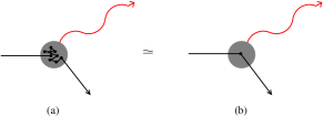
Figure 5: A non-relativistic example of the probability for soft bremsstrahlung radiation being unable to resolve details of charge particle tracks that are smaller than the photon wavelength.

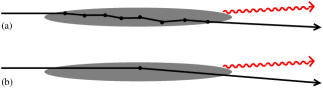
Figure 6: The same processes as Fig. 5, now viewed from a highly boosted reference frame. The deflection angles are very small and the bremsstrahlung nearly collinear, but I have exaggerated the angles for the purpose of drawing the picture.

In the high energy case, photon bremsstrahlung will be nearly collinear with the charged particle, which can be understood as a result of the boost. In the ultra-relativistic limit, closer collinearity means larger formation lengths. Another useful mnemonic to keep in mind is that a photon emitted at angle $\theta$ from an ultra-relativistic particle is not very sensitive to particle deflections small compared to $\theta$. So the photon emission angle will be less than or order the net deflection angle of the charged particle within the formation length.

Fig. 7 is somewhat similar to Fig. 6 but shows the case of propagation through a medium whose size is small compared to the formation length. The start of the particle trajectory corresponds to whatever hard process (not shown) originally launched the high-energy particle in its approximate direction of motion. Bremsstrahlung photons cannot resolve the difference between Fig. 7a and Fig. 7b, and so the medium does not have a significant effect on the probability of bremsstrahlung.

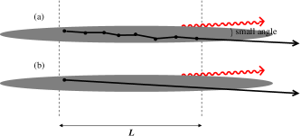
Figure 7: The equivalence of bremsstrahlung (a) with and (b) without medium interactions for the case where the length $L$ of medium traversed is small compared to the formation length.

Now consider the case of rarer collisions that involve a single larger-than-typical elastic scattering, as in Fig. 8a. This scattering can then affect bremsstrahlung radiation at larger than usual angles, corresponding to photons with smaller formation times. If the angle is large enough, so that the formation length in that particular case becomes smaller than the $O(L)$ distance between the rare collision and the start of the particle’s trajectory, then the photon can resolve the difference between Fig. 8a and 8b. The rare collision is therefore a second chance for bremsstrahlung, independent of the original event that produced the high-energy particle and without any LPM suppression. As far as this photon is concerned, the process is similar to the $N{=}1$ process shown in Fig. 8c.

Because of the relatively small formation length, some readers may wonder if the additional typical-angle scattering events in Fig. 8a can provide additional, distinct opportunities for bremsstrahlung, as depicted in Fig. 9, and so ruin the equivalence of Figs. 8a and 8c. This does not happen because the short-formation-length photons we have considered in the rare scattering case of Fig. 8 are emitted at angles large compared to the typical net scattering angle during one such formation length. The scatterings shown in the two additional ovals of Fig. 9, for example, do not produce significant bremsstrahlung radiation at such large angles.

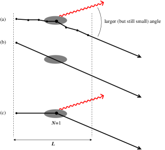
Figure 8: Like Fig. 7, but now (a) there is a rare scattering with larger than typical deflection angle, which affects bremsstrahlung at larger angles, which corresponds to smaller formation length (shaded ovals). Case (b) is no longer approximately (a), but case (c) is.

Figure 9: As Fig. 8 but considering the possibility of similar photon production from other, typical collisions along the trajectory. This possibility is suppressed.

The upshot of this discussion is that scattering with larger than usual angles is rarer but, when it does happen, the probability for an associated bremsstrahlung photon is higher because there is less LPM suppression. Which type of process dominates the medium effect on bremsstrahlung depends on which of these opposing effects on probability is the most important.

II.2 Review of LPM Effect

For QED, one of the usual approaches to qualitative estimates of the formation length is the following: two space-time points $X_{1}$ and $X_{2}$ on the charged particle’s trajectory lie within one formation length if the relative phase $K_{\mu}(X_{1}-X_{2})^{\mu}$ for photon emission from those two points is $\ll 1$. If the particle is moving nearly linearly at close to the speed of light, this condition becomes $\omega\,|{\bm{x}}_{1}{-}{\bm{x}}_{2}|(1-\cos\theta)\ll 1$, where $\theta$ is the angle between the photon and the charged particle. Changing $\ll$ to $\sim$ then qualitatively defines the formation length $l_{\rm f}$, which for small $\theta$ gives $\omega l_{\rm f}\theta^{2}\sim 1$ and so

$$l_{\rm f}\sim\frac{1}{\omega\theta^{2}}.$$ (23)

A more general way to the same result is to consider how off-shell in energy the intermediate particle line is in a simple bremsstrahlung diagram like Fig. 10, which is

$$\delta E\equiv E_{s}({\bm{p}})+E_{\gamma}({\bm{k}})-E_{s}({\bm{p}}+{\bm{k}})\simeq\frac{p_{\perp}^{2}+m_{s}^{2}}{2p}+\frac{k_{\perp}^{2}+m_{\gamma}^{2}}{2k}-\frac{|{\bm{p}}_{\perp}+{\bm{k}}_{\perp}|^{2}+m_{s}^{2}}{2(p+k)}\,,$$ (24)

where ${\bm{P}}={\bm{p}}+{\bm{k}}$ is the original momentum and the $m$ are the effective finite-temperature masses of the particles. The formation time is the quantum mechanical duration of the off-shell state, $l_{\rm f}\sim(\delta E)^{-1}$. If one ignores the masses, (24) can be rewritten in the form

$$l_{\rm f}\sim\frac{1}{\delta E}\sim\frac{p+k}{pk\bigl{(}\frac{p_{\perp}}{p}-\frac{k_{\perp}}{k}\bigr{)}^{2}}\simeq\frac{1}{x(1-x)E\theta^{2}}\,.$$ (25)

For $x$ not too close to 1 (i.e. $1{-}x$ not small), this is the same parametric estimate as (23). As stated earlier, I will focus on $x<1/2$ and ignore the case of small $1{-}x$ in the main text.

Figure 10: One of the diagrams contributing to simple bremsstrahlung from a single scattering from the plasma. (The other important diagram is the one where the bremsstrahlung comes from the initial high-energy particle line.)

Now, to set some scales, consider QED bremsstrahlung in an infinite medium, which is dominated by typical scattering events. The dominant photons are those whose angle $\theta$ relative to the charged particle is of order the net deflection angle $\Delta\theta$ of the charged particle from the scatterings it experiences during one formation time: Bremsstrahlung at larger angles $\theta\gg\Delta\theta$ is suppressed. On the other hand, because of multiple collisions, the average angle $\theta$ that the photon makes with the charged particle during a formation time cannot be smaller than order $\Delta\theta$. So (23) becomes

$$l_{\infty}\sim\frac{1}{\omega(\Delta\theta)^{2}}\,.$$ (26)

In an infinite medium (or any medium larger than the formation length), the typical deflection angle $\Delta\theta$ of the charged particle in one formation length $l_{\infty}$ is

$$(\Delta\theta)_{\infty}\sim\frac{Q_{\perp\rm\infty}}{E}\sim\frac{(\hat{q}l_{\infty})^{1/2}}{E}\,,$$ (27)

where $Q_{\perp\infty}\sim(\hat{q}l_{\infty})^{1/2}$ is the transverse momentum the charged particle picks up over that distance. Combining (26) and (27),

$$l_{\infty}(\omega)\sim\sqrt{\frac{E^{2}}{\hat{q}\omega}}\,.$$ (28)

Energy loss in an infinite medium is dominated by the case $\omega\sim E$ where the photon carries away a significant fraction of the particle’s energy. In this case, the formation length becomes $L_{\infty}\sim\sqrt{E/\hat{q}}$, just like the QCD result quoted in (1).

For the sake of easy reference, and for comparing and contrasting QED and QCD bremsstrahlung, I have collected in Table 1 some of the formulas described here and in section III.

	QED	QCD
$l_{\rm f}$	$\frac{1}{\omega\theta^{2}}\sim\frac{1}{\omega(\Delta\theta)^{2}}$	$\frac{1}{\omega\theta^{2}}\sim\frac{1}{\omega(\Delta\theta)_{\rm g}^{2}}$	formation length (general)
$\theta$	$\Delta\theta\sim\frac{Q_{\perp}}{E}$	$(\Delta\theta)_{\rm g}\sim\frac{Q_{\perp}}{\omega}$	characteristic bremsstrahlung angle
$(Q_{\perp}^{2})_{\rm typ}$ for $L\lesssim l_{\infty}$	$\hat{q}L$	$\hat{q}_{\rm A}L$	typical momentum transfer
$l_{\infty}(\omega)$	$\sqrt{\frac{E^{2}}{\hat{q}\omega}}$	$\sqrt{\frac{\omega}{\hat{q}_{\rm A}}}$	infinite-medium formation length
$L_{\infty}\sim l_{\infty}(E/2)$	$\sqrt{\frac{E}{\hat{q}}}$	$\sqrt{\frac{E}{\hat{q}}}$	dominant $l_{\infty}$ for energy loss
$\hat{q}$	$\alpha^{2}n\ln\left(\frac{\hat{q}L}{m_{\rm D}^{2}}\right)$	$\hat{q}_{\rm A}\sim C_{\rm A}\alpha^{2}{\cal N}\ln\left(\frac{\hat{q}_{\rm A}L}{m_{\rm D}^{2}}\right)$	relevant $Q_{\perp}^{2}$ per length

Table 1: Summary of various parametric formulas for the LPM effect in QED and QCD. These formulas assume $1{-}x$ is not small, and the QCD formulas ignore the difference between $\hat{q}_{\rm A}$ and $\hat{q}_{\rm F}$ in the case $\omega\sim E$.

II.3 Bremsstrahlung for a given $Q_{\perp}$

Let $Q_{\perp}$ be the total transverse momentum transferred to the charged particle as it traverses a medium of length $L$, and consider the case $L\ll l_{\infty}(\omega)$ of a medium that is thin compared to the typical infinite-volume formation length (28) for photons with some frequency $\omega$. In this section, I will focus on how the medium effect on the bremsstrahlung probability depends on $Q_{\perp}$.

II.3.1 LPM suppression in thin media

Consider a charged, nearly massless particle that undergoes a single scattering in vacuum. The probability that this scattering will produce a photon with frequency of order $\omega$ (for any $\omega\lesssim E$) is of order $\alpha$ times a collinear logarithm. For the vacuum case, integration over bremsstrahlung frequencies gives rise to an additional, infrared logarithm in the probability. In considering medium effects on bremsstrahlung, I am going to delay integration over frequency until the end and will for now just consider the probability of emission of photons whose frequencies are of order some scale $\omega$. The collinear logarithm comes from integrating over photon directions that are very close to either the incoming or outgoing particle track in an isolated collision. It plays only a limited role in medium effects on bremsstrahlung. For the moment, I will ignore the collinear logarithm and simply take $\alpha$ to be the additional cost in probability of emitting a photon of frequency $\sim\omega$ when there is a collision. The angle this photon makes with the incoming and outgoing particle tracks is of order the deflection angle of the particle track, with discussion of the possibility of more-nearly collinear photons deferred to later discussion of the collinear logarithm.

In a medium, divide the multiple collisions along a trajectory into sets which are each roughly one formation length long. The photon cannot resolve the difference of a single vs. multiple collision in each set, but it does see each set as a distinct opportunity for bremsstrahlung. There is then an $O(\alpha)$ probability for a photon emission from each set for which $\Delta\theta\sim\theta$. So, for instance, the shaded oval in Fig. 8a is associated with a probability of $O(\alpha)$ [times a collinear logarithm] for emitting a bremsstrahlung photon at the angle shown.

In Fig. 7a, there is also an $O(\alpha)$ probability of emitting such a photon at the angle $\theta\sim\Delta\theta$ shown there. But the difference in emission probability with the vacuum case of Fig. 7b is small. In this case, I will write the medium contribution to the $O(\alpha)$ probability of photon emission as $O(\epsilon\alpha)$, where $\epsilon$ is an LPM suppression factor due to the photon’s failure to resolve (i) the collisions in the medium from (ii) the event that originally created the charged particle:

$$\Delta(\mbox{cost of bremsstrahlung emission})\sim\epsilon\alpha.$$ (29)

Fig. 11 shows the behavior of $\epsilon$ as a function of $Q_{\perp}^{2}$. I will explain this figure one feature at a time.

Figure 11: Suppression factor $\epsilon$ of medium effects as a function of $Q_{\perp}^{2}$ for the case where the medium thickness $L$ is smaller than the typical formation length $l_{\infty}(\omega)$ of the infinite-medium case.

For a given scattering trajectory—e.g. the typical scattering events of Fig. 7a or the rare events of 8a, or something in between—the relevant formation length will depend on the deflection angle, which for thin media will be related to the net transverse momentum transfer $Q_{\perp}$ while traversing the medium by

$$\Delta\theta\sim\frac{Q_{\perp}}{E}.$$ (30)

The corresponding formation length (23) is

$$l_{\rm f}\sim\frac{1}{\omega(\Delta\theta)^{2}}\sim\frac{E^{2}}{\omega Q_{\perp}^{2}}\,.$$ (31)

Note that in a rare scattering case like Fig. 8a, I should have estimated the formation length based on the net deflection over the formation length, shown by the shaded oval, rather then from the deflection over the entire trajectory. However, in this case, the rare scattering dominated the total angular deflection in any case, and so I do not need to distinguish between the two.

The region $\epsilon\simeq 1$ of Fig. 11 corresponds to cases $l_{\rm f}\ll L$ where the scattering process looks like Fig. 8a rather than Fig. 7a. From (31), this condition is equivalent to

$$Q_{\perp}^{2}\gg\frac{E^{2}}{\omega L}\qquad\mbox{for $\epsilon\simeq 1$}.$$ (32)

II.3.2 The size of $\epsilon$

Now turn to the case $Q_{\perp}^{2}\ll E^{2}/\omega L$ where the formation time $l_{\rm f}$ of (31) is large compared to $L$, corresponding to situations like Fig. 7a. Recall that the LPM effect occurs when the relative phase $K_{\mu}(X_{1}-X_{2})^{\mu}$ is small for space-time points $X_{1}$ and $X_{2}$ corresponding to collisions. For collisions spread out over a distance $L$ as in Fig. 7a, this relative phase is of order $\omega L(1-\cos\theta)\sim\omega L\theta^{2}$. We have LPM suppression if $\omega L\theta^{2}\ll 1$, and the amount of LPM suppression of the effects of collisions with the medium turns out to be given by the square of this relative phase:

$$\epsilon\sim(K\cdot\Delta X)^{2}\sim(\omega L\theta^{2})^{2}\sim\left(\frac{L}{l_{\rm f}}\right)^{2}.$$ (33)

I give a brief review in Appendix B.1 of why this is the amount of suppression. Putting the formation length (31) into (33),

$$\epsilon\sim\frac{\omega^{2}L^{2}}{E^{4}}\,Q_{\perp}^{4},$$ (34)

as depicted by the fall-off of $\epsilon$ with decreasing $Q_{\perp}$ shown in Fig. 11.

For $Q_{\perp}^{2}$ small compared to the typical transfer of $(Q_{\perp}^{2})_{\rm typ}\sim\hat{q}L$, the solid line in Fig. 11 deviates from (34), with the latter indicated by a dotted line. This qualitative difference will not matter to the eventual conclusions of this paper, but I will take a moment to explain it for the sake of completeness. In earlier discussion, I slightly oversimplified when asserting that bremsstrahlung is suppressed if the photon angle $\theta$ is large compared to the net deflection angle $\Delta\theta\sim Q_{\perp}/E$ of the charged particle. Consider the trajectory shown in Fig. 12. Here, the net deflection of the trajectory is zero but the intermediate deflection is non-zero. The typical bremsstrahlung photon angle is then of order the intermediate deflection angle, which I show in more detail in Appendix B.2. Now consider cases of many multiple scatterings within a formation time. The rare cases where $N$ multiple scatterings produce smaller-than-typical deflections are dominated by situations where the first $N/2$ scatterings produce a typical deflection, which by random chance was nearly canceled by an opposite deflection from the second $N/2$ scatterings. The dominant photon angle $\theta$ will then be determined by the intermediate deflection $\sim(Q_{\perp})_{\rm typ}/E$ rather then the total deflection $\sim Q_{\perp}/E$ that was used in (30) and (31). The upshot is that $Q_{\perp}\ll(Q_{\perp})_{\rm typ}$ collisions behave just like $Q_{\perp}\sim(Q_{\perp})_{\rm typ}$ collisions in terms of the medium effect on bremsstrahlung.

Figure 12: Example of two scatterings with zero total deflection angle.

II.3.3 Putting it together

For a thin medium, we can now find a parametric result for the medium effect $\Delta P_{\rm brem}$ on the probability of single-photon bremsstrahlung for photons of frequency $\sim\omega$ through scattering processes with total momentum transfer $\sim Q_{\perp}$. Neglecting collinear logarithms, it is simply the probability of the underlying scattering event times a factor of $\epsilon\alpha$ for the associated bremsstrahlung. Multiplying (i) Fig. 1 for $dP_{\rm scatt}/d(Q_{\perp}^{2})$ times (ii) Fig. 11 for $\epsilon$ times (iii) $\alpha$ gives

$$\frac{d(\Delta P_{\rm brem})}{d(Q_{\perp}^{2})}\sim\frac{dP_{\rm scatt}}{d(Q_{\perp}^{2})}\times\epsilon(\omega,Q_{\perp}^{2})\times\alpha,$$ (35)

which is depicted in Fig. 13a. There is an additional logarithmic factor shown for the high-$Q_{\perp}$ tail in Fig. 13a that is not included in the product (35). This is a collinear logarithm that I will explain in a moment. Recall that the notation $\Delta P_{\rm brem}$ is defined in terms of the frequency spectrum by (21).

Figure 13: Medium modification to probability for emitting a high-energy bremsstrahlung gluon of frequency $\sim\omega$: probability distribution vs. $Q_{\perp}^{2}$. In (b), $Q_{\perp}$ represents the transverse momentum picked up in a distance $l_{\infty}(\omega)$.

Fig. 13b shows the corresponding result for a thick medium $L\gg l_{\infty}(\omega)$. Since relevant formation lengths in this case will not exceed $l_{\infty}(\omega)$, we can break the problem up into independent probabilities for each section of medium of length $l_{\infty}$. For a section of length $l_{\infty}$, we have $\epsilon\sim 1$. So (35) is modified to

$$\frac{d(\Delta P_{\rm brem})}{d(Q_{\perp}^{2})}\sim\frac{L}{l_{\infty}(\omega)}\times\left[\frac{dP_{\rm scatt}}{d(Q_{\perp}^{2})}\right]_{L=l_{\infty}(\omega)}\times\alpha,$$ (36)

where here $Q_{\perp}$ refers to the transverse momentum transfer over a length of order $l_{\infty}(\omega)$. The parametric behaviors shown in Figs. 13a and b agree for the dividing case of $L\sim l_{\infty}(\omega)$.

When discussing “thick” media, I have implicitly assumed that a single bremsstrahlung analysis of the medium effect remains adequate. In particular, the media should be small compared to the stopping distance for the high-energy particle: $L\ll L_{\infty}/\alpha$. The stopping distance is where $\Delta E\sim E$, as can be read off from Fig. 3 for QCD or later from Fig. 17 for QED.

II.3.4 Collinear logarithms

I will now discuss collinear logarithms associated with bremsstrahlung, which were ignored in the previous analysis. For simplicity, consider the case $\omega\ll E$ of soft bremsstrahlung, where the charged particle trajectory can be thought of as a classical source for the electromagnetic field. For further simplicity, start by considering a trajectory corresponding to exactly one scattering from the medium, as in Fig. 8c, rather than more complicated trajectories like Figs. 8a or 7a that include multiple small-angle scatterings. In this case, there is a collinear logarithm in the bremsstrahlung probability associated with small photon angles $\theta\ll\Delta\theta$ relative to the final particle direction, as in Fig. 14a. There is also potentially a similar logarithm associated with collinearity with the initial particle direction, as in Fig. 14b, but this second logarithm can be suppressed by the LPM effect.

Figure 14: (a) initial and (b) final state collinear radiation from a single scattering with the medium. For comparison, (c) shows the case of collinear radiation when there are no medium collisions but only the initial hard scattering event that created the high-energy particle moving in the same final direction.

Throughout this discussion, I will assume that $E$ and $\omega$ are large enough compared to effective masses that I can treat the charged particle and photon as massless. So I will not keep track of the cut-off of collinear logarithms due to masses.

In the case of final-state collinearity shown in Fig. 14a, the enhancement of the bremsstrahlung probability at small angles is the same as that for the vacuum process of Fig. 14c. There is therefore no corresponding collinear logarithm in the medium effect $\Delta P_{\rm brem}$, which expresses the difference between the two. More detail is given in Appendix B.1.

Now consider collinearity with the earlier direction of the particle trajectory, as in Fig. 14b, and let $\theta_{{\rm i}\gamma}$ be the small angle that the photon makes with that direction. The corresponding collinear logarithm will be cut off at small $\theta_{{\rm i}\gamma}$ when the formation length (31) becomes large compared to the length of that segment of the trajectory, because then the photon cannot resolve the difference between the particle trajectories of Figs. 14b and 14c. A generic collision in the medium will be a distance of order $L$ from the start, and so the angles which contribute to a collinear logarithm must satisfy $l_{\rm f}(\theta_{{\rm i}\gamma})\lesssim L$, which is

$$\frac{1}{\omega\theta_{{\rm i}\gamma}^{2}}\lesssim L.$$ (37)

The angles which contribute to the collinear logarithm are therefore

$$\sqrt{\frac{1}{L\omega}}\lesssim\theta_{{\rm i}\gamma}\lesssim\Delta\theta.$$ (38)

The collinear logarithm appears when there exists such a hierarchy of angular scales, and it is then

$$\ln\left(\frac{(\Delta\theta)^{2}}{(\theta_{{\rm i}\gamma})_{\rm min}^{2}}\right)\sim\ln\left(\frac{\omega LQ_{\perp}^{2}}{E^{2}}\right).$$ (39)

This is the logarithmic factor shown on the large $Q_{\perp}^{2}$ tail of Fig. 13a. The range (38) only exists if $Q_{\perp}^{2}\gg E^{2}/\omega L$.

So far, I have considered single scattering processes like Fig. 14a–b rather than actual cases of interest to this paper, such as Fig. 8a. The angle that the photon makes with the trajectory preceding the relatively large angle collision in Fig. 8a is smeared out by multiple soft scatterings, which deflected the particle by an angle of order $(Q_{\perp})_{\rm typ}/E\sim\sqrt{\hat{q}L/E^{2}}$. The angular range (38) contributing to a collinear logarithm is then replaced by

$$\max\left(\sqrt{\frac{1}{\omega L}}\,,\sqrt{\frac{\hat{q}L}{E^{2}}}\right)\lesssim\theta_{{\rm i}\gamma}\lesssim\Delta\theta.$$ (40)

The first case on the left-hand side dominates when $L\ll l_{\infty}(\omega)$, as in Fig. 13a. For $L\gg l_{\infty}(\omega)$, the relevant length scale is $l_{\infty}(\omega)$ rather than $L$, and the logarithm becomes

$$\ln\left(\frac{(\Delta\theta)^{2}}{(\theta_{{\rm i}\gamma})_{\rm min}^{2}}\right)\sim\ln\left(\frac{Q_{\perp}^{2}}{\hat{q}\,l_{\infty}(\omega)}\right).$$ (41)

This is argued in more detail in Appendix B.3. The logarithmic factor (41) is the one shown on the large $Q_{\perp}^{2}$ tail of Fig. 13b.

Now return to the case of final-state radiation in a case like Fig. 8a. Once the particle leaves the medium, there is always a semi-infinite straight line segment of the trajectory to which a photon can become collinear. So, unlike the case just considered, the effect of multiple soft scatterings before the particle leaves the medium cannot suppress the production of final-state collinear photons: photons can be produced at arbitrarily small angles (if the charged particle is treated as massless) by being produced after the very last scattering in the medium. But this contribution cancels when we subtract the vacuum contribution to get $\Delta P_{\rm brem}$, just as discussed earlier for the case of Fig. 14a.

II.4 Bremsstrahlung spectrum and energy loss

I now want to integrate over $Q_{\perp}^{2}$ to find the spectrum $\Delta P_{\rm brem}=\omega\>d(I-I_{\rm vac})/d\omega$ as a function of $\omega$. To see visually what values of $Q_{\perp}$ dominate the integration, it is useful to multiply the previous results of Fig. 13 by a factor of $Q_{\perp}^{2}$ so that $d(\Delta P_{\rm brem})/d(Q_{\perp}^{2})$ becomes the logarithmic derivative $Q_{\perp}^{2}\>d(\Delta P_{\rm brem})/d(Q_{\perp}^{2})$. The result is shown in Fig. 15. In the thin-media case, there are two peaks, corresponding to two different $Q_{\perp}$ scales that will give the dominant contributions to the integral. One scale is the scale $Q_{\perp}^{2}\sim\hat{q}L$ of typical scattering events, corresponding to HO processes like Fig. 7a. The formation length $l_{\rm f}$ in this case is large compared to $L$. The other, larger $Q_{\perp}$ scale corresponds to rarer, larger-angle scattering events that are well approximated by the $N=1$ approximation and which have a shorter formation length than the typical scattering events. The scale $Q_{\perp}^{2}\sim E^{2}/\omega L$ of the right-hand peak in Fig. 15a corresponds to the case where this shorter formation length is of order $L$. The tail at yet larger $Q_{\perp}$ corresponds to yet shorter formation lengths, as were depicted in Fig. 8. This tail falls off because no further gains are made in the suppression factor $\epsilon$ by further decreasing $l_{\rm f}$ below $L$, but the probability of the underlying scattering event decreases.

Figure 15: This is Fig. 13 multiplied by $Q_{\perp}^{2}$. (a) assumes that $l_{\infty}(\omega)/\sqrt{\log}\ll L\ll l_{\infty}(\omega)$; the figure is similar for $L\ll l_{\infty}(\omega)/\sqrt{\log}$, but then the right-hand ($N{=}1$) peak would be the higher one.

Which of the peaks of Fig. 15a dominates in the thin-media case of $L\ll l_{\infty}(\omega)$ depends on the exactly how small $L$ is. The HO and $N{=}1$ peak heights are

$$\Delta P_{\rm brem}(\omega)\sim\frac{\alpha\hat{q}^{2}\omega^{2}L^{4}}{E^{4}}\sim\alpha\left(\frac{L}{l_{\infty}(\omega)}\right)^{4}\hskip 70.0001pt(\mbox{HO})$$ (42)

and

$$\Delta P_{\rm brem}(\omega)\sim\frac{\alpha^{3}n\omega L^{2}}{E^{2}}\sim\frac{\alpha}{\ln(\hat{q}L/m_{\rm D}^{2})}\left(\frac{L}{l_{\infty}(\omega)}\right)^{2}\hskip 40.00006pt(N{=}1)$$ (43)

respectively. The $N{=}1$ peak dominates when

$$L\ll\frac{l_{\infty}(\omega)}{\bigl{[}\ln(\hat{q}L/m_{\rm D}^{2})\bigr{]}^{1/2}}\,.$$ (44)

The $Q_{\perp}$-integrated result $\Delta P_{\rm brem}$ is of order the highest peak in Fig. 15. The result is shown vs. $L$ in Fig. 4, provided one takes the QED formula (28) for $l_{\infty}=l_{\infty}(\omega)$ instead of (22).

Now consider the dependence on $\omega$ when $L$ is fixed. This behavior is shown in Fig. 16 except that I multiply by an extra factor of $\omega$ to plot the contribution

$$\omega\,\frac{d(\Delta E)}{d\omega}=\omega^{2}\,\frac{d}{d\omega}(I-I_{\rm vac})=\omega\,\Delta P_{\rm brem}(\omega)$$ (45)

to the medium effect on average energy loss from photons with frequency $\sim\omega$.

Fig. 16c shows the case for thick media $L\gg L_{\infty}$, where $L_{\infty}$ is given by (1) and represents the typical formation length for the case $\omega\sim E$. In QED (unlike QCD), the typical formation length $l_{\infty}(\omega)$ given by (28) grows with decreasing $\omega$. For $\omega$ relatively large, $l_{\infty}(\omega)$ will still exceed $L$, and $\Delta P_{\rm brem}$ will be given by the peak height

$$\Delta P_{\rm brem}(\omega)\sim\alpha\,\frac{L}{l_{\infty}(\omega)}\sim\frac{\alpha L\sqrt{\hat{q}\omega}}{E}$$ (46)

of Fig. 15b. When multiplied by $\omega$, this gives the corresponding formula shown on the right of Fig. 16c. This formula works until $\omega$ gets small enough that $l_{\infty}(\omega)\sim L$, which occurs at $\omega\sim E^{2}/\hat{q}L^{2}$. For smaller $\omega$, first the HO peak and then the $N{=}1$ peak of Fig. 15a will determine $\Delta P_{\rm brem}$, giving (42) and (43) respectively, corresponding to the other formulas shown in Fig. 16c.

Figure 16: Medium modification to QED energy loss $\Delta E$: contribution of bremsstrahlung photons with frequency $\sim\omega$.

In the case of $L\ll L_{\infty}$, shown in Figs. 16a and b, we always have $l_{\infty}(\omega)\gg L$, and one or more of the stages just described are bypassed.

Finally, integrating over $\omega$, the total medium contribution $\Delta E$ to average energy loss just corresponds parametrically to the maximum in Fig. 16. A sketch of the resulting dependence of $\Delta E$ on medium thickness $L$ is shown in Fig. 17. This result is qualitatively different from the QCD result previewed in Fig. 3, for reasons which will be explained in the next section. The $L^{2}$ dependence of the QED result for sufficiently small $L$ has been discussed previously by Peigné and Smilga PeigneSmilga .

Figure 17: Total medium modification to QED energy loss $\Delta E$, shown vs. medium length $L$.

III Bremsstrahlung in QCD

III.1 Review of LPM Effect in QCD

The major difference between bremsstrahlung in QCD and QED is that a bremsstrahlung gluon carries charge and so, like the particle that radiated, can also $t$-channel scatter from the medium. It is easier to deflect a lower momentum particle than a higher momentum particle and so, for the case $\omega\ll E$, it is scattering of the gluon rather than the original particle that dominates determination of the angle $\theta$ between the two. The medium effect on bremsstrahlung is therefore dominated by

$$\theta\sim(\Delta\theta)_{\rm g}\sim\frac{Q_{\perp}}{\omega}\,,$$ (47)

instead of the corresponding QED angle (30). Correspondingly, here $Q_{\perp}$ is the transverse momentum that the bremsstrahlung gluon, rather than the original particle, picks up in a formation time. For the case $\omega\sim E$, the deflections (47) and (30) of the gluon and the original particle are parametrically the same size, up to details of group Casimirs related to whose $Q_{\perp}$ we consider, which I will not bother to distinguish in my parametric estimates in this case. So I will use (47) for the entire range $\omega\lesssim E$, assuming as always that $1{-}x$ is not small.

The formation length corresponding to (23) and (31) is then

$$l_{\rm f}\sim\frac{1}{\omega(\Delta\theta)_{\rm g}^{2}}\sim\frac{\omega}{Q_{\perp}^{2}}\,.$$ (48)

The argument for the size of the formation length $l_{\infty}(\omega)$ in an infinite medium then goes through just as in (26–28) for the QED case, but with $\Delta\theta$ and $E$ replaced by $(\Delta\theta)_{\rm g}$ and $\omega$, so that

$$l_{\infty}(\omega)\sim\sqrt{\frac{\omega}{\hat{q}_{\rm A}}}\,,$$ (49)

as quoted earlier in (22). The main qualitative difference between QCD and QED bremsstrahlung in a medium is that the QCD formation length $l_{\infty}(\omega)$ decreases in the soft limit of decreasing $\omega$ due to the ease with which a soft gluon is deflected, whereas in QED $l_{\infty}(\omega)$ increases with decreasing $\omega$.

III.2 Bremsstrahlung spectrum and energy loss

The analysis of the $Q_{\perp}$ dependence of the bremsstrahlung problem is basically the same as in QED, but with the modifications described above concerning the formation length. The QCD versions of Figs. 11, 13 and 15 are given by 18–20. The only change in these figures is the replacement of $E$ by $\omega$ and the clarification that $\hat{q}$ is $\hat{q}_{\rm A}$ in the case $\omega\ll E$. There are group factors associated with each power of $\alpha$, but I will not keep track of these in the figures. (Similarly, I will not distinguish between ${\cal N}$ and the density $n$ in figures.) The nature of the collinear logarithm in the QCD case is reviewed in Appendix C.

A quick check can be made of the parametric estimate $\epsilon\sim\hat{q}_{\rm A}^{2}L^{4}/\omega^{2}$ shown in Fig. 18a for typical scatterings $Q_{\perp}^{2}\sim(Q_{\perp}^{2})_{\rm typ}$ for thin media. The medium effect on the bremsstrahlung probability is then of order

$$C_{s}\alpha\epsilon\sim\frac{C_{s}\alpha\hat{q}_{\rm A}^{2}}{\omega^{2}}\,L^{4}$$ (50)

by (29), where here I’ve included the factor of $C_{s}$ associated with the $\alpha$ for the coupling of the bremsstrahlung gluon. Typical scatterings are described by the HO approximation, and (50) correctly reproduces the parametric dependence of the known HO result (8) for the thin media modification to the spectrum of gluon bremsstrahlung.

Now return to the general problem. Evaluating the integration over $Q_{\perp}$ by the peak heights in Fig. 20, the dependence of the medium modification $\Delta P_{\rm brem}$ on medium thickness $L$, for bremsstrahlung gluons with a frequency of order $\sim\omega$, is given in Fig. 4, but this time with the QCD value (49) for $l_{\infty}(\omega)$ instead of the QED version.

Figure 18: The QCD analog of Fig. 11 for the suppression factor $\epsilon$.

Figure 19: The QCD analog of Fig. 13 for the bremsstrahlung probability dependence on $Q_{\perp}$.

Figure 20: The QCD analog of Fig. 15. For $L\ll l_{\infty}(\omega)/\sqrt{\log}$, the right-hand peak in (a) is the higher one.

From the peak heights of Fig. 20 or equivalently from the results for $\Delta P_{\rm brem}(\omega)$ in Fig. 4, one may extract Fig. 21 showing the medium effect on the energy loss spectrum as a function of frequency $\omega$. This figure is qualitatively very different from the QED version of Fig. 16 because of the qualitative difference in $l_{\infty}(\omega)$. In QED, small $\omega$ leads to larger formation lengths and so more LPM suppression, which is why the QED figure was dominated by $\omega$ of order the largest scale, $\omega\sim E$. In QCD, small $\omega$ leads to smaller formation lengths and so less LPM suppression, which is why for thin media the QCD figure has significant contributions from $\omega\ll E$.

Figure 21: Medium modification to QCD energy loss $\Delta E$: contribution of bremsstrahlung gluons with frequency $\sim\omega$. This is the QCD analog of Fig. 16.

Figs. 21b–c show that the typical scattering processes captured by the HO approximation dominate (at leading-log order) not only for length $L$ large compared to the typical infinite-medium formation length $L_{\infty}$, but also in the entire range $L\gg L_{\infty}/\sqrt{\log}$, which includes $L\sim L_{\infty}$. For the case $L\ll L_{\infty}/\sqrt{\log}$ of Fig. 21a, the situation is more complicated. Obtaining the total $\Delta E$ corresponds to integrating the curve in Fig. 21 with $d(\ln\omega)=d\omega/\omega$. The peak in Fig. 21a gives an HO-dominated contribution of order the peak height,

$$C_{s}\alpha\hat{q}_{\rm A}L^{2}\sim C_{s}C_{\rm A}\alpha^{3}{\cal N}L^{2}\ln\left(\frac{\hat{q}_{\rm A}L}{m_{\rm D}^{2}}\right)\qquad\mbox{(HO contribution).}$$ (51)

The long flat plateau at larger $\omega$ gives a contribution of order the height of the plateau times a logarithm of its range:

$$C_{s}C_{\rm A}\alpha^{3}{\cal N}L^{2}\times\int_{\sim\hat{q}_{\rm A}L^{2}\log}^{\sim E}\frac{d\omega}{\omega}\sim C_{s}C_{\rm A}\alpha^{3}{\cal N}L^{2}\ln\left(\frac{E}{\hat{q}_{\rm A}L^{2}}\right).$$ (52)

Over the frequency range $\hat{q}_{\rm A}L^{2}\log\ll\omega\ll E$ of this plateau, the value of $\omega\>d(\Delta E)/d\omega$ is well approximated by the $N{=}1$ approximation, with the scattering events which dominate the medium effect having the form of Fig. 2b. Adding the two contributions (51) and (52) together gives the final result (18) quoted in the introduction. As described there, the HO contribution continues to dominate the $N{=}1$ contribution for $L$ all the way down until the $L_{*}\sim(m_{\rm D}^{4}/\hat{q}_{\rm A}E)^{1/6}L_{\infty}$ of (20). This is parametrically very different from the QED case of Fig. 17, where HO processes dominate $\Delta E$ only down until $L\sim L_{\infty}/\sqrt{\log}$.

It is important to note that there is no ($N{=}1$)-like contribution for $\omega\ll\hat{q}_{\rm A}L^{2}$ in Fig. 3a that is separate from the HO contribution and that would parametrically reduce the lower scale $\hat{q}_{\rm A}L^{2}$ in the logarithm of (52) to make the sum (18) of (51) and (52) larger. To check, I will estimate the contribution $\delta(\Delta E)$ to $\Delta E$ from ($N{=}1$)-like scattering (Fig. 2b) with $\omega\lesssim\hat{q}_{\rm A}L^{2}$, as opposed to HO-like scattering (Fig. 2a). The range $\omega\ll\hat{q}_{\rm A}L^{2}$ in Fig. 21 corresponds to $L\gg l_{\infty}(\omega)$ and so to Fig. 20b. The contribution to $\Delta P_{\rm brem}$ from the $N{=}1$ part of that curve is of order the height in Fig. 20b where the HO and $N{=}1$ curves meet:

$$\delta(\Delta P_{\rm brem})\sim\frac{C_{s}\alpha}{\ln(\hat{q}_{\rm A}L/m_{\rm D}^{2})}\,\frac{L}{l_{\infty}(\omega)}\sim\frac{C_{s}\alpha L}{\ln(\hat{q}_{\rm A}L/m_{\rm D}^{2})}\sqrt{\frac{\hat{q}_{\rm A}}{\omega}}\,.$$ (53)

Multiplying by $\omega$ and integrating over the range $\omega\lesssim\hat{q}_{\rm A}L^{2}$ under discussion gives an additional $N{=}1$ contribution to $\Delta E$ of

$$\delta(\Delta E)\sim\Bigl{[}\omega\,\delta(\Delta P_{\rm brem})\Bigr{]}_{\omega\sim\hat{q}_{\rm A}L^{2}}\sim\frac{C_{s}\alpha\hat{q}_{\rm A}L^{2}}{\ln(\hat{q}_{\rm A}L/m_{\rm D}^{2})}\sim C_{s}C_{\rm A}\alpha^{3}{\cal N}L^{2}.$$ (54)

This contribution from $(N{=}1)$-like events with $\omega\lesssim\hat{q}_{\rm A}L^{2}$ is sub-leading in logarithms compared to the HO contribution (51) and the total result (18), and so it can be ignored in a leading-log analysis.

IV Comparison to Zakharov’s Analysis

IV.1 The Puzzle

In Ref. ZakharovResolution , Zakharov argued that the HO approximation should be expected to break down when $L$ is less than or order the infinite-volume formation time. In this paper, I have argued that the HO approximation does a little better than that if one consistently treats logarithms as large. For the case of the medium modification to the bremsstrahlung spectrum, depicted in Fig. 20, the HO approximation dominates as long as $L\gg l_{\infty}(\omega)/\sqrt{\log}$, which includes $L\sim l_{\infty}(\omega)$. In this section, I will paraphrase Zakharov’s argument and resolve the slight difference in conclusion.

First, I need to briefly review the formalism for doing a full calculation of the gluon bremsstrahlung spectrum BSZ , which was originally developed for finite media by Baier, Dokshitzer, Mueller, Peigne, and Schiff BDMPS1 ; BDMPS2 ; BDMPS3 ; BDMS and by Zakharov Zakharov1 ; Zakharov2 . A brief summary in my own notation, which is suited for discussing problems where the particles in the medium are not fixed scatterers, can be found in Ref. timelpm1 . The spectrum is given by timelpm1

$$\omega\,\frac{d}{d\omega}(I-I_{\rm vac})=\frac{\alpha x\,P_{s{\to}{\rm g}}(x)}{[x(1-x)E]^{2}}\,\operatorname{Re}\int_{0}^{\infty}dt_{1}\int_{t_{1}}^{\infty}dt_{2}\>\\ \Bigl{[}{\bm{\nabla}}_{{\bm{B}}_{1}}\cdot{\bm{\nabla}}_{{\bm{B}}_{2}}\bigl{\{}G({\bm{B}}_{2},t_{2};{\bm{B}}_{1},t_{1})-G_{\rm vac}({\bm{B}}_{2},t_{2};{\bm{B}}_{1},t_{1})\bigr{\}}\Bigr{]}_{B_{1}=B_{2}=0},$$ (55)

where $G({\bm{B}}_{2},t_{2};{\bm{B}}_{1},t_{1})$ is the Green’s function for a two-dimensional quantum mechanics problem with the time-dependent, non-hermitian Hamiltonian

$$H(t)=\delta E({\bm{p}}_{B})-i\Gamma_{3}({\bm{B}},t).$$ (56)

Here $\delta E$ describes the energy difference $(E_{s,{\bm{p}}}+E_{{\rm g},{\bm{k}}})-E_{s,{\bm{p}}+{\bm{k}}}$ between (i) a high-energy parton of momentum ${\bm{P}}={\bm{p}}+{\bm{k}}$ and energy $E=P$ and (ii) the same parton with momentum ${\bm{p}}$ plus a bremsstrahlung gluon with momentum ${\bm{k}}$. In the high-energy limit, if we ignore masses, it can be written as

$$\delta E({\bm{p}}_{B})\simeq\frac{p_{B}^{2}}{2x(1-x)P}\equiv\frac{p_{B}^{2}}{2M}$$ (57)

where ${\bm{p}}_{B}\equiv(p{\bm{k}}_{\perp}-k{\bm{p}}_{\perp})/P$ is the transverse momentum conjugate to the ${\bm{B}}$ of (56) and $M\equiv x(1-x)P$ is the “mass” of the two-dimensional Schrödinger problem:

$$H(t)\simeq\frac{p_{B}^{2}}{2M}-i\Gamma_{3}({\bm{B}},t).$$ (58)

For fixed $x$, this ${\bm{p}}_{B}$ is proportional to the angle between ${\bm{k}}$ and ${\bm{p}}$. The second term in (58) is

$$\Gamma_{3}({\bm{B}},t)=\tfrac{1}{2}C_{\rm A}\,\bar{\Gamma}_{2}({\bm{B}},t)+(C_{s}-\tfrac{1}{2}C_{\rm A})\,\bar{\Gamma}_{2}(x{\bm{B}},t)+\tfrac{1}{2}C_{\rm A}\,\bar{\Gamma}_{2}\bigl{(}(1-x){\bm{B}},t\bigr{)},$$ (59)

where

$$\bar{\Gamma}_{2}({\bm{b}},t)\equiv\int d^{2}q_{\perp}\>\frac{d\bar{\Gamma}_{\rm el}(t)}{d^{2}q_{\perp}}\,(1-e^{i{\bm{b}}\cdot{\bm{q}}_{\perp}}).$$ (60)

Here $\bar{\Gamma}_{\rm el}$ is defined by $\Gamma_{\rm el}\equiv C_{R}\bar{\Gamma}_{\rm el}$. That is, it is the elastic scattering rate without the group factor $C_{R}$ associated with the particle being scattered.

The high-energy limit corresponds to large mass $M$ in the two-dimensional Hamiltonian (58) and so will be determined by the small $B$ behavior of the “potential” $-i\Gamma_{3}({\bm{B}},t)$. Naively, (60) for small $b$ gives

$$\bar{\Gamma}_{2}({\bm{b}},t)\simeq\hat{\bar{q}}b^{2},$$ (61)

where $C_{R}\hat{\bar{q}}$ is formally the average momentum transfer per unit length rather than the typical transfer used throughout this paper. The actual small $b$ behavior of $\Gamma_{2}$ is proportional to $b^{2}\ln(m_{\rm D}^{2}b^{2})$, not $b^{2}$, which is reflected by the UV divergence of the integral (11) for average transverse momentum transfer. Cutting off this divergence by replacing $C_{R}\hat{\bar{q}}$ by the typical momentum transfer per unit length, as in (13b), corresponds to the harmonic oscillator approximation, so named because of the form of (61).

In contrast, another analytic approach to solving the problem is to keep the full original form of (58) and instead do perturbation theory in powers of the (imaginary-valued) potential $-i\Gamma_{3}$. This is the formal version of the opacity expansion.

Alternatively, both approximations can be made. Consider the case of the brick problem. If one first makes the HO approximation (61) and then makes the opacity expansion, the opacity expansion is simply the expansion of the HO result (5) in powers of $|\omega_{0}^{2}|\propto\hat{\bar{q}}\propto-i\Gamma_{3}$:

$$\omega\,\frac{d}{d\omega}(I-I_{\rm vac})_{\rm HO}=\frac{\alpha}{\pi}\,x\,P_{s{\to}{\rm g}}(x)\,\left[\tfrac{1}{12}|\omega_{0}|^{4}L^{4}-\tfrac{17}{2520}|\omega_{0}|^{8}L^{8}+\cdots\right].$$ (62)

Parametrically, this expansion has the form

$$\omega\,\frac{d}{d\omega}(I-I_{\rm vac})_{\rm HO} \sim C_{s}\alpha\left[\#\left(\frac{\hat{q}_{\rm A}L^{2}}{\omega}\right)^{2}+\#\left(\frac{\hat{q}_{\rm A}L^{2}}{\omega}\right)^{4}+\cdots\right]$$

$$\sim C_{s}\alpha\left[\#\left(\frac{L^{2}}{[l_{\infty}(\omega)]^{2}}\right)^{2}+\#\left(\frac{L^{2}}{[l_{\infty}(\omega)]^{2}}\right)^{4}+\cdots\right]$$

$$\sim C_{s}\alpha\left[\#\left(\frac{C_{\rm A}\alpha^{2}{\cal N}L^{2}\log}{\omega}\right)^{2}+\#\left(\frac{C_{\rm A}\alpha^{2}{\cal N}L^{2}\log}{\omega}\right)^{4}+\cdots\right],$$ (63)

with the logarithms defined as in (16). The condition for the perturbative expansion of (61) to be useful is that successive terms get smaller and smaller, which parametrically is the condition that $L\ll l_{\infty}(\omega)$. As noted by Zakharov ZakharovResolution , there is no first-order term (no term proportional to $\omega_{0}^{2}$ and so proportional to the interaction $\Gamma_{3}$) in the expansion (62). But if $L\ll l_{\infty}(\omega)$ so that a perturbative treatment of the quantum mechanical problem is valid, then why not forgo the HO approximation and just use the full, original potential $-i\Gamma_{3}$. At first order, one then obtains the $N{=}1$ result (9), so that

$$\omega\,\frac{d}{d\omega}(I-I_{\rm vac})\sim C_{s}\alpha\left[\#\,\frac{C_{\rm A}\alpha^{2}{\cal N}L^{2}}{\omega}+\cdots\right].$$ (64)

The fact that a perturbative expansion of the HO result should work whenever $L\ll l_{\infty}(\omega)$, yet the HO approximation is clearly missing the first-order term in this limit, makes it seem like the HO approximation must be untrustworthy whenever $L\ll l_{\infty}(\omega)$.

IV.2 Reconciliation

The absence of the first-order term in the expansion of the HO result can be illuminated if one separates out from Eq. (55) the step of taking the real part. The origin of the HO result (5) is actually

$$\omega\,\frac{d}{d\omega}(I-I_{\rm vac})_{\rm HO}=\frac{\alpha}{\pi}\,x\,P_{s{\to}{\rm g}}(x)\,\operatorname{Re}\left[\ln\cos(\omega_{0}L)\right].$$ (65)

Correspondingly, using $\omega_{0}^{2}=-i|\omega_{0}|^{2}$, the perturbative expansion is

$$\omega\,\frac{d}{d\omega}(I-I_{\rm vac})_{\rm HO}=\frac{\alpha}{\pi}\,x\,P_{s{\to}{\rm g}}(x)\,\operatorname{Re}\left[\tfrac{i}{2}|\omega_{0}|^{2}L^{2}+\tfrac{1}{12}|\omega_{0}|^{4}L^{4}+\tfrac{i}{45}|\omega_{0}|^{6}L^{6}-\tfrac{17}{2520}|\omega_{0}|^{8}L^{8}+\cdots\right],$$ (66)

which shows the missing odd terms in the expansion. This corresponds to

$$\omega\,\frac{d}{d\omega}(I-I_{\rm vac})_{\rm HO}\sim C_{s}\alpha\operatorname{Re}\left[i\,\#\frac{C_{\rm A}\alpha^{2}{\cal N}L^{2}}{\omega}\ln\left(\frac{\hat{q}_{\rm A}L}{m_{\rm D}^{2}}\right)+\#\left(\frac{C_{\rm A}\alpha^{2}{\cal N}L^{2}\log}{\omega}\right)^{2}+\cdots\right]$$ (67)

In contrast, the full $N{=}1$ perturbative calculation turns out to give

$$\omega\,\frac{d}{d\omega}(I-I_{\rm vac})_{N{=}1} \simeq\frac{C_{\rm A}\alpha^{3}{\cal N}}{\omega}\,L^{2}\,x\,P_{s{\to}{\rm g}}(x)\,\operatorname{Re}\left[i\ln\left(\frac{m_{\rm D}^{2}L}{\#iM}\right)\right]$$

$$=\frac{C_{\rm A}\alpha^{3}{\cal N}}{\omega}\,L^{2}\,x\,P_{s{\to}{\rm g}}(x)\,\operatorname{Re}\left[i\ln\left(\frac{m_{\rm D}^{2}L}{\#M}\right)+\frac{\pi}{2}\right]$$ (68)

in the limit of large logarithms. Taking the real part and the small $x$ limit, this reproduces (9). Parametrically,

$$\omega\,\frac{d}{d\omega}(I-I_{\rm vac})_{N{=}1} \sim C_{s}\alpha\operatorname{Re}\left[i\,\#\frac{C_{\rm A}\alpha^{2}{\cal N}L^{2}}{\omega}\ln\left(\frac{m_{\rm D}^{2}}{i\omega}\right)\right]$$

$$\sim C_{s}\alpha\operatorname{Re}\left[i\#\frac{C_{\rm A}\alpha^{2}{\cal N}L^{2}}{\omega}\left\{\ln\left(\frac{m_{\rm D}^{2}}{\omega}\right)-i\#\right\}\right]$$ (69)

Comparing (67) and (69) before taking the real part, note that the first-order terms are parametrically the same except that the arguments of the large logarithms are different. When the real part is taken, however, nothing survives of the first term in the expansion (67) of the HO result, but a term sub-leading in large logarithms survives from the $N{=}1$ result. The moral is that the structure of the $N{=}1$ and HO results for thin media are not very different before one takes the real part. After the real part, a calculation which included contributions from both HO and $N{=}1$ physics, as described in this paper, would be expected to produce a result of the form

$$\omega\,\frac{d}{d\omega}(I-I_{\rm vac})_{\rm HO}\sim C_{s}\alpha\left[\frac{C_{\rm A}\alpha^{2}nL^{2}}{\omega}+\#\left(\frac{C_{\rm A}\alpha^{2}{\cal N}L^{2}\log}{\omega}\right)^{2}+\cdots\right]$$ (70)

This is consistent with the $L\lesssim l_{\infty}(\omega)$ behavior of $\Delta P_{\rm brem}$ found in this paper and shown in Fig. 4.

IV.3 Some Differences

It is important to note, however, that a perturbative calculation to second order in $-i\Gamma_{3}$ would not give precisely (70) with the HO logarithm (16),

$$\log\equiv\ln\left(\frac{\hat{q}_{\rm A}L}{m_{\rm D}^{2}}\right)\sim\ln\left(\frac{C_{\rm A}\alpha^{2}{\cal N}L}{m_{\rm D}^{2}}\right).$$ (71)

When discussing the perturbative expansion (63) of the HO result, I first made the HO approximation (61) and treated $\hat{\bar{q}}$ as a constant given by (13b). Only then did I expand in powers of $-i\Gamma_{3}$. If I instead forgo the HO approximation, then the expansion in $-i\Gamma_{3}$ (the opacity expansion) is equivalent to an expansion in powers of the medium density $\sim{\cal N}$, if for this purpose I treat the Debye screening mass $m_{\rm D}$ as a variable independent from ${\cal N}$. However, (70) is not a simple power series expansion in ${\cal N}$, because there is a factor of ${\cal N}$ inside the argument to the logarithm (71). The second-order HO term in (70) can therefore only arise from a resummation of many terms of the opacity expansion.

In this paper, I will not attempt to explore in detail how physics associated with the HO approximation can be seen to arise from resummation of terms in the opacity expansion. But I hope that the discussion of this section gives some insight into how the earlier results of this paper, based on more physical arguments, can be consistent formally with the small $L$ expansions of the $N{=}1$ and HO approximations.

Appendix A The form of $dP_{\rm scatt}/d(Q_{\perp}^{2})$

The qualitative form of Fig. 1 — a diffusion peak from typical scatterings with a single-scattering tail due to rare scatterings — has a very long history. For example, a simplified version of Molliere’s theory of multiple scattering was given by Bethe in 1953 Bethe . In the current context of leading-log approximations to jet $Q_{\perp}$ broadening in quark-gluon plasmas, it has been addressed previously in Sec. 3.1 of Ref. BDMPS3 and is nicely reviewed in Appendix A of Ref. PeigneSmilga for the particular model of scattering where $d\Gamma_{\rm el}/d(q_{\perp}^{2})$ is taken to be proportional to $(q_{\perp}^{2}+m_{\rm D}^{2})^{-2}$. For the sake of completeness, I will review here the important elements for the current work in a model-independent way. Specifically, the important points for my argument in this paper are that (i) $dP_{\rm scatt}/d(Q_{\perp}^{2})\sim 1/\hat{q}L$ for $Q_{\perp}^{2}\ll\hat{q}L$ (the peak height in Fig. 1), and (ii) $dP_{\rm scatt}/d(Q_{\perp}^{2})\sim\alpha^{2}nL/Q_{\perp}^{4}$ for $Q_{\perp}^{2}\gg\hat{q}L$ (the form of the large $Q_{\perp}$ tail).

The transition between these two behaviors occurring for $\hat{q}L\lesssim Q_{\perp}^{2}\lesssim\hat{q}L\ln(\log)$ in Fig. 1 is interesting but unimportant to my conclusions. In this paper, I treat logarithms as large but I treat logarithms of logarithms $\ln(\log)$ as $O(1)$. So $Q_{\perp}^{2}\gg\hat{q}L$ refers to the tail of Fig. 1 and not to any part of the transition region.

Though not needed for the present work, I will also provide reference to a rigorous mathematical generalization of the central limit theorem which demonstrates that the soft-scattering peak indeed approaches a Gaussian form in the limit of a large number of collisions.

A.1 Review of general multiple scattering formula

Let

$$f(Q_{\perp},t)\equiv\frac{dP_{\rm scatt}}{d^{2}Q_{\perp}}=\frac{1}{\pi}\frac{dP_{\rm scatt}}{d(Q_{\perp}^{2})}$$ (72)

be the two-dimensional probability distribution of ${\bm{Q}}_{\perp}$ at time $t$. I follow the standard development of multiple scattering by writing the evolution equation for $f$, which is

$$\partial_{t}f({\bm{Q}}_{\perp},t)=\int_{{\bm{q}}_{\perp}}\rho({\bm{q}}_{\perp})[f({\bm{Q}}_{\perp}{-}{\bm{q}}_{\perp},t)-f({\bm{Q}}_{\perp},t)]$$ (73)

in a uniform medium, where

$$\rho(q_{\perp})\equiv\frac{d\Gamma_{\rm el}({\bm{q}}_{\perp})}{d^{2}q_{\perp}}$$ (74)

is the two-dimensional probability density for acquiring a transverse momentum kick of ${\bm{q}}_{\perp}$ in a single, individual collision. The first term on the right-hand side of (73) is a gain term, representing momentum change from ${\bm{Q}}_{\perp}{-}{\bm{q}}_{\perp}$ to ${\bm{Q}}_{\perp}$. The second term is a loss term, representing change from ${\bm{Q}}_{\perp}$ to ${\bm{Q}}_{\perp}{+}{\bm{q}}_{\perp}$. Take the initial condition $f({\bm{Q}}_{\perp},0)=\delta^{(2)}({\bm{Q}}_{\perp})$. The equation is solved by Fourier transformating to

$$\partial_{t}\tilde{f}({\bm{b}},t)=[\tilde{\rho}({\bm{b}})-\tilde{\rho}(\bm{0})]f({\bm{b}},t)$$ (75)

with initial condition $\tilde{f}({\bm{b}},0)=1$ and solution

$$\tilde{f}({\bm{b}},t)=e^{-[\tilde{\rho}(\bm{0})-\tilde{\rho}({\bm{b}})]t}.$$ (76)

Fourier transforming back,

$$\frac{dP_{\rm scatt}}{d^{2}Q_{\perp}}=\int_{{\bm{b}}}e^{-[\tilde{\rho}(\bm{0})-\tilde{\rho}({\bm{b}})]t}e^{-i{\bm{b}}\cdot{\bm{Q}}_{\perp}},$$ (77)

where

$$\tilde{\rho}(\bm{0})-\tilde{\rho}({\bm{b}})=\int_{{\bm{q}}_{\perp}}\frac{d\Gamma_{\rm el}({\bm{q}}_{\perp})}{d^{2}q_{\perp}}(1-e^{i{\bm{b}}\cdot{\bm{q}}_{\perp}}).$$ (78)

A.2 Examples

As an example, consider the weak-coupling result AGK

$$\frac{d\Gamma_{\rm el}}{d^{2}q_{\perp}}\simeq\frac{C_{R}g^{2}Tm_{\rm D}^{2}}{(2\pi)^{2}q_{\perp}^{2}(q_{\perp}^{2}+m_{\rm D}^{2})}$$ (79)

which holds for $q_{\perp}\ll T$. The result is not significantly different for $q_{\perp}\gg T$ ArnoldDogan ; ArnoldXiao , so I shall take it as an example for discussing the entire range of $q_{\perp}$. The $1/q_{\perp}^{2}$ behavior for $q_{\perp}\ll m_{\rm D}$ is due to magnetic scattering, which is not completely screened by the Debye effect. The Fourier transform of (79) gives AMYimpact

$$\tilde{\rho}(\bm{0})-\tilde{\rho}(\bm{b})=\frac{C_{R}g^{2}T}{2\pi}\left[K_{0}(m_{\rm D}b)-\ln\left(\frac{2}{m_{\rm D}b}\right)+\gamma_{\rm E}\right].$$ (80)

Note that for $m_{\rm D}b\ll 1$ this becomes

$$\tilde{\rho}(\bm{0})-\tilde{\rho}({\bm{b}})\simeq\frac{C_{R}g^{2}T}{8\pi}(m_{\rm D}b)^{2}\left[\ln\left(\frac{2}{m_{\rm D}b}\right)-\gamma_{\rm E}+1\right],$$ (81)

and for $m_{\rm D}b\gg 1$ it is

$$\tilde{\rho}(\bm{0})-\tilde{\rho}({\bm{b}})\simeq\frac{C_{R}g^{2}T}{2\pi}\left[-\ln\left(\frac{2}{m_{\rm D}b}\right)+\gamma_{\rm E}\right]\to+\infty\quad\mbox{as $b\to\infty$.}$$ (82)

Alternatively, consider a popular model used in this subject, which is

$$\frac{d\Gamma_{\rm el}}{d^{2}q_{\perp}}\to\frac{C_{R}g^{4}{\cal N}}{(2\pi)^{2}(q_{\perp}^{2}+m_{\rm D}^{2})^{2}},$$ (83)

where ${\cal N}$ is the number density weighted by appropriate group factors. Fourier transforming, one finds

$$\tilde{\rho}({\bm{b}})=\frac{C_{R}g^{4}{\cal N}}{4\pi m_{\rm D}}\,b\,K_{1}(m_{\rm D}b),$$ (84)

so that

$$\tilde{\rho}(\bm{0})-\tilde{\rho}({\bm{b}})=\frac{C_{R}g^{4}{\cal N}}{4\pi m_{\rm D}^{2}}\,\left[1-m_{\rm D}b\,K_{1}(m_{\rm D}b)\right].$$ (85)

For $m_{\rm D}b\ll 1$,

$$\tilde{\rho}(\bm{0})-\tilde{\rho}({\bm{b}})\simeq\frac{C_{R}g^{4}{\cal N}}{8\pi}\,b^{2}\left[\ln\left(\frac{2}{m_{\rm D}b}\right)-\gamma_{\rm E}+\frac{1}{2}\right],$$ (86)

and for $m_{\rm D}b\gg 1$ it is

$$\tilde{\rho}(\bm{0})-\tilde{\rho}({\bm{b}})\simeq\tilde{\rho}(\bm{0})=\frac{C_{R}g^{4}{\cal N}}{4\pi m_{\rm D}^{2}}\qquad\mbox{as $b\to\infty$.}$$ (87)

The $b^{2}\ln(m_{\rm D}b)$ at small $b$ in both examples is a universal result of having a $d\Gamma_{\rm el}/d^{2}q_{\perp}$ that falls as $1/q_{\perp}^{4}$ at large $q_{\perp}$. This in turn is a universal feature of point-particle scattering that is Coulomb at short distances. Note that the two formulas (81) and (86) have the same size parametrically, so it does not matter which we use if we are interested in a parametric analysis. In general,

$$\tilde{\rho}(\bm{0})-\tilde{\rho}({\bm{b}})\sim C_{R}g^{4}{\cal N}b^{2}\ln\left(\frac{1}{m_{\rm D}b}\right)\quad\mbox{for $m_{\rm D}b\ll 1$.}$$ (88)

In the second example, the finite $b{\to}\infty$ limit (87) means that the final Fourier transform (77) used to obtain $dP_{\rm scatt}/d^{2}Q_{\perp}$ contains a $\delta$-function singularity. This can be isolated by rewriting (77) as

$$\frac{dP_{\rm scatt}}{d^{2}Q_{\perp}}=e^{-\tilde{\rho}(\bm{0})\,t}\delta^{(2)}({\bm{b}})+\int_{{\bm{b}}}\left[e^{-[\tilde{\rho}(\bm{0})-\tilde{\rho}({\bm{b}})]t}-e^{-\tilde{\rho}(\bm{0})\,t}\right]e^{-i{\bm{b}}\cdot{\bm{Q}}_{\perp}}.$$ (89)

The coefficient of the $\delta$-function is just the probability $\exp(-\Gamma_{\rm el}t)$ that there are no scatterings whatsoever. For large $\Gamma_{\rm el}t$ this can be ignored. This $\delta$-function does not appear in the first example (79) since in that case $\Gamma_{\rm el}=\int_{{\bm{q}}_{\perp}}d^{2}\Gamma_{\rm el}/d^{2}q_{\perp}=\infty$ because of the $1/q_{\perp}^{2}$ infrared behavior of (79) due to magnetic scattering. Either way, I will ignore the $\delta$ function in the rest of this discussion.

A.3 The height of the peak

For the height of the peak if Fig. 1, we just need to evaluate the regular (i.e. non-$\delta$-function) term in (89) at $Q_{\perp}{=}0$:

$$\left(\frac{dP_{\rm scatt}}{d^{2}Q_{\perp}}\right)^{\rm reg}_{Q_{\perp}=0}=\int_{{\bm{b}}}\left[e^{-[\tilde{\rho}(\bm{0})-\tilde{\rho}({\bm{b}})]t}-e^{-\tilde{\rho}(\bm{0})\,t}\right].$$ (90)

For large enough $t$, this integral is dominated by small $b$ determined by $[\tilde{\rho}(\bm{0})-\tilde{\rho}({\bm{b}})]t\sim 1$. Using (88), this is

$$C_{R}g^{4}{\cal N}tb^{2}\ln\left(\frac{1}{m_{\rm D}b}\right)\sim 1,$$ (91)

and so

$$b^{2}\sim\left[C_{R}g^{4}{\cal N}t\ln\left(\frac{C_{R}g^{4}{\cal N}t}{m_{\rm D}^{2}}\right)\right]^{-1}\sim\frac{1}{\hat{q}_{R}t}.$$ (92)

The condition $m_{\rm D}b\ll 1$ that I have used is then satisfied provided $t\gg m_{\rm D}^{2}/(C_{R}g^{4}{\cal N})$, which, neglecting group factors, is of order $1/g^{2}T$. This is just the condition that there are many $q_{\perp}{\sim}m_{\rm D}$ scatterings, which I have assumed throughout this paper. From (92), the size of the integral (90) is then

$$\left(\frac{dP_{\rm scatt}}{d^{2}Q_{\perp}}\right)^{\rm reg}_{Q_{\perp}=0}\sim b^{2}\sim\frac{1}{\hat{q}_{R}t}.$$ (93)

Replacing $t$ by $L$, this is just the peak height depicted in Fig. 1.

The $Q_{\perp}{=}0$ result will be a good approximation whenever the $\exp(i{\bm{b}}\cdot{\bm{Q}}_{\perp})$ factor in (89) is approximately 1 up to and including $b$ values of order (92). So $dP_{\rm scatt}/d^{2}Q_{\perp}\sim 1/\hat{q}_{R}L$ for $Q_{\perp}\ll b^{-1}\sim\sqrt{\hat{q}_{R}L}$, just as shown in Fig. 1. For larger $Q_{\perp}$, the oscillating factor will cause $dP_{\rm scatt}/d^{2}Q_{\perp}$ to fall. For much larger $Q_{\perp}$, the oscillating factor $\exp(i{\bm{Q}}_{\perp}\cdot b_{\perp})$ causes the integral in (89) to be dominated by even smaller $b$, in which case one may approximate

$$e^{-[\tilde{\rho}(\bm{0})-\tilde{\rho}({\bm{b}})]t}\simeq 1-[\tilde{\rho}(\bm{0})-\tilde{\rho}({\bm{b}})]t.$$ (94)

Completing the Fourier transform, this just gives that the large $Q_{\perp}$ behavior of $d\Gamma/d^{2}Q_{\perp}$ is given by the single-scattering formula $d\Gamma_{\rm el}/d^{2}q_{\perp}$ with ${\bm{q}}_{\perp}={\bm{Q}}_{\perp}$, producing the tail of Fig. 1.

A.4 The Gaussian shape of the peak

Ref. BDMPS3 discusses the Gaussian shape of the peak by noting that $\ln(b^{2})$ is a slowly varying function and so making the approximation of replacing this logarithm by a constant in (89). This is the harmonic oscillator approximation and gives a Gaussian result for $dP_{\rm scatt}/d^{2}Q_{\perp}$. Ref. BDMPS3 notes that this approximation breaks down for the tail, which is generated by the non-analyticity of $\ln b$ at $b{=}0$. Some readers may wonder, however, if the argument that the shape approaches Gaussian can be made more rigorous. If the distribution $d^{2}\Gamma_{\rm el}/q^{2}q_{\perp}$ of single-scattering rates had a finite variance $\langle q_{\perp}^{2}\rangle<\infty$, then the the approach to a Gaussian shape would be guaranteed by the central limit theorem. Finite variance is a sufficient condition for the central limit theorem, but it is not a necessary condition. A necessary and sufficient condition may be found in Theorem 8.1.3 of Ref. Meerschaert . I will simplify their condition to the radially-symmetric case of interest here. Using the notation of this paper, the condition can be written in terms of the truncated variance

$$\hat{q}_{\Lambda}\equiv\int_{{\bm{q}}_{\perp}}({\bm{q}}_{\perp}\cdot\bm{n})^{2}\,\rho(q_{\perp})\,\theta(\Lambda-|{\bm{q}}_{\perp}\cdot\bm{n}|)),$$ (95)

where $\theta(z)$ is the step function, ${\bm{q}}_{\perp}$ could be a vector of any dimension, $\rho({\bm{q}}_{\perp})$ is a probability density in that vector space, $\Lambda$ is a cut-off, and $\bm{n}$ is a unit vector in any direction. The necessary and sufficient condition for the central limit theorem is that

$$\lim_{\Lambda\to\infty}\frac{\hat{q}_{\lambda\Lambda}}{\hat{q}_{\Lambda}}=1$$ (96)

for all $\lambda>0$. This condition applies to the case relevant in this paper, where $\hat{q}_{\Lambda}\propto\ln\Lambda$ in the limit of large $\Lambda$.

Appendix B More details on suppression $\epsilon$ in QED

B.1 Review: Why $\epsilon\sim(K\cdot\Delta x)^{2}$ in QED

Here I will briefly review the parametric formula (33) for the suppression factor $\epsilon$. For simplicity, I will focus on QED in the soft bremsstrahlung limit, $\omega\ll E$. In this limit, the charged particle trajectory can be thought of as a fixed, classical source $J^{\mu}(t,{\bm{x}})$ for the electromagnetic field, and the bremsstrahlung amplitude is proportional to the Fourier transform $J^{\mu}(\omega,{\bm{k}})$. For further simplicity, I will focus on a comparison of a single scattering from the medium, as in Figs. 14a–b, with the vacuum case of Fig. 14c.

The Fourier transform $J^{\mu}(K)$ of the current for the trajectory shown in Figs. 14a-b is

$$J^{\mu}(K) \propto\frac{V_{\rm i}^{\mu}}{K\cdot V_{\rm i}}(e^{iK\cdot X_{0}}-e^{iK\cdot X_{1}})+\frac{V_{\rm f}^{\mu}}{K\cdot V_{\rm f}}\,e^{iK\cdot X_{1}}$$

$$=e^{iK\cdot X_{1}}\left[\frac{V_{\rm i}^{\mu}}{K\cdot V_{\rm i}}(e^{-iK\cdot\Delta X}-1)+\frac{V_{\rm f}^{\mu}}{K\cdot V_{\rm f}}\right],$$ (97)

where $K=(\omega,{\bm{k}})=(k,{\bm{k}})$ is the photon 4-momentum, and $V\equiv(1,{\bm{v}})$ with the charged particle velocity ${\bm{v}}$ before ($V_{\rm i}$) and after ($V_{\rm f}$) the medium collision. The medium effect on the bremsstrahlung probability is then

$$|\varepsilon\cdot J|^{2}-|\varepsilon\cdot J|_{\rm vac}^{2}\propto\left|\frac{\varepsilon\cdot V_{\rm i}}{K\cdot V_{\rm i}}(e^{-iK\cdot\Delta X}-1)+\frac{\varepsilon\cdot V_{\rm f}}{K\cdot V_{\rm f}}\right|^{2}-\left|\frac{\varepsilon\cdot V_{\rm f}}{K\cdot V_{\rm f}}\right|^{2},$$ (98)

where $\varepsilon^{\mu}$ is the photon polarization. The first term in (98) corresponds to Figs. 14a–b and the second to Fig. 14c. Expanding the first square and summing over polarizations gives

$$\sum_{\varepsilon}\left[|\varepsilon\cdot J|^{2}-|\varepsilon\cdot J|_{\rm vac}^{2}\right]\propto 2\left[1-\cos(K\cdot\Delta X)\right]\sum_{\varepsilon}\operatorname{Re}\left[\frac{\varepsilon^{*}\cdot V_{\rm i}}{K\cdot V_{\rm i}}\left(\frac{\varepsilon\cdot V_{\rm i}}{K\cdot V_{\rm i}}-\frac{\varepsilon\cdot V_{\rm f}}{K\cdot V_{\rm f}}\right)\right].$$ (99)

For $K\cdot\Delta X\ll 1$, the bremsstrahlung probability is therefore proportional to $(K\cdot\Delta X)^{2}$, as in (33).

The $\epsilon\sim(K\cdot\Delta X)^{2}$ suppression factor favors larger photon angles relative to $\Delta{\bm{x}}$ over smaller ones. So it’s important to review what sets the upper limit on photon angle in the current context. The difference (99) between the bremsstrahlung probabilities in medium and in vacuum will sometimes be positive and sometimes negative. Consider the average of (99) over rotations of the direction of ${\bm{v}}_{\rm f}$ around the axis defined by ${\bm{v}}_{1}$. Let $\theta_{\gamma 1}$ and $\theta_{{\rm f}1}$ be the angles that ${\bm{k}}$ and ${\bm{v}}_{\rm f}$ makes with ${\bm{v}}_{\rm 1}$, and let $\phi_{{\rm f}1}$ represent the azimuthal angle being averaged over. Ignore mass effects, so that ${\bm{v}}_{\rm f}$ is a unit vector. The averaging gives

$$\left\langle\frac{\varepsilon\cdot V_{\rm f}}{K\cdot V_{\rm f}}\right\rangle_{\rm\phi_{{\rm f}1}}=\frac{\varepsilon\cdot V_{1}}{K\cdot V_{1}}\qquad\mbox{if $\theta_{\gamma 1}>\theta_{{\rm f}1}$},$$ (100)

where $\langle\cdots\rangle_{\phi_{{\rm f}1}}$ indicates averaging over $\phi_{{\rm f}1}$. So the corresponding average of the medium effect (99) vanishes if $\theta_{\gamma 1}$ is larger than the deflection angle $\Delta\theta=\theta_{{\rm f}1}$ of the charged particle trajectory in Fig. 14. For multiple scatterings involving a number of consecutive trajectory directions ${\bm{v}}_{1}$, ${\bm{v}}_{2}$, …, ${\bm{v}}_{N}={\bm{v}}_{\rm f}$, one can start by averaging over rotations of ${\bm{v}}_{N}$ about ${\bm{v}}_{\rm N-1}$ and then work back recursively to show that a similar cancellation occurs if $\theta_{\gamma,n{-}1}>\theta_{n,n{-}1}$ for all $n$.

Eqs. (98) and (99) also show the behavior associated with collinear logs discussed in Section II.3.4. Compare (99) to the usual calculation of bremsstrahlung from an isolated collision like Fig. 22:

$$|\varepsilon\cdot J|^{2}\propto\left|-\frac{\varepsilon\cdot V_{\rm i}}{K\cdot V_{\rm i}}+\frac{\varepsilon\cdot V_{\rm f}}{K\cdot V_{\rm f}}\right|^{2}.$$ (101)

The collinear divergences associated with photons collinear with the initial or final direction correspond to the divergence of (101) as $K\cdot V_{\rm i}$ or $K\cdot V_{\rm f}$ vanishes, respectively. If polarizations are summed over, this corresponds to divergences like $1/\theta^{2}_{{\rm i}\gamma}$ and $1/\theta^{2}_{{\rm f}\gamma}$, where $\theta_{{\rm i}\gamma}$ and $\theta_{{\rm f}\gamma}$ are the corresponding angles. Integration over angles $d^{2}\Omega$ then gives the usual collinear logarithmic divergences. In (98), however, the cancellation with the vacuum term softens the $K\cdot V_{\rm f}\to 0$ behavior, so that there is no corresponding logarithmic divergence in the angular integration. The other divergence, $K\cdot V_{\rm i}\to 0$, is cut off once $K\cdot\Delta X\propto K\cdot V_{\rm i}$ becomes small enough that $1-\cos(K\cdot\Delta X)\sim(K\cdot\Delta X)^{2}$ in (99): that is, when $K\cdot\Delta X\ll 1$.

Figure 22: An isolated collision.

B.2 The case $Q_{\perp}\ll(Q_{\perp})_{\rm typ}$

The diagram of Fig. 12 corresponds to

$$J^{\mu}(K) \propto-\frac{V_{\rm i}^{\mu}}{K\cdot V_{\rm i}}\,e^{iK\cdot X_{1}}+\frac{V_{1}^{\mu}}{K\cdot V_{1}}(e^{iK\cdot X_{1}}-e^{iK\cdot X_{2}})+\frac{V_{\rm f}^{\mu}}{K\cdot V_{\rm f}}\,e^{iK\cdot X_{2}}$$

$$=e^{iK\cdot X_{2}}\left(\frac{V_{1}^{\mu}}{K\cdot V_{1}}-\frac{V_{\rm i}^{\mu}}{K\cdot V_{\rm i}}\right)(e^{-iK\cdot\Delta X}-1),$$ (102)

where $V_{1}$ is the intermediate particle direction and the initial and final directions are equal: $V_{\rm i}=V_{\rm f}$. So

$$|\varepsilon\cdot J|^{2}\propto\left|-\frac{\varepsilon\cdot V_{\rm i}}{K\cdot V_{\rm i}}+\frac{\varepsilon\cdot V_{1}}{K\cdot V_{1}}\right|^{2}\left|e^{-iK\cdot\Delta X}-1\right|^{2}.$$ (103)

The factor $|e^{-iK\cdot\Delta X}-1|^{2}$ gives $\epsilon\sim(K\cdot\Delta X)$ LPM suppression when $K\cdot\Delta X\ll 1$. The other factor in (103) looks just like the result (101) that the individual collisions would each give if they were isolated. The two terms in this factor approximately cancel each other only when the photon angle is large compared to the angle between $V_{\rm i}=V_{\rm f}$ and $V_{1}$. In order of magnitude, the characteristic angle $\theta$ of bremsstrahlung from two collisions with canceling deflections is therefore similar to that of two collisions with deflections in the same direction.

B.3 Collinear logarithms for thick media

Here I will flesh out the argument for the collinear logarithm (41) that appears for the high-$Q_{\perp}$ tail in Fig. 13b in the thick medium case $L\gg l_{\infty}(\omega)$. Return to Eq. (40). Multiple scatterings preceding the rare, larger-than-typical angle scattering will only affect the bremsstrahlung process if they occur within the corresponding mean free time $l_{\rm f}(\theta_{{\rm i}\gamma})\sim 1/\omega\theta_{{\rm i}\gamma}^{2}$. So, the condition (41) should more accurately be written

$$\max\left(\sqrt{\frac{1}{\omega L}}\,,\sqrt{\frac{\hat{q}\min[L,l_{\rm f}(\theta_{{\rm i}\gamma})]}{E^{2}}}\right)\lesssim\theta_{{\rm i}\gamma}\lesssim\Delta\theta.$$ (104)

For $L\gg l_{\infty}(\omega)$, the lower bound on $\theta_{{\rm i}\gamma}$ which dominates is

$$\sqrt{\frac{\hat{q}\,l_{\rm f}(\theta_{{\rm i}\gamma})}{E^{2}}}\sim\sqrt{\frac{\hat{q}}{\omega E^{2}\theta_{{\rm i}\gamma}^{2}}}\lesssim\theta_{{\rm i}\gamma}.$$ (105)

This is equivalent to

$$\left(\frac{\hat{q}}{\omega E^{2}}\right)^{1/4}\lesssim\theta_{{\rm i}\gamma}.$$ (106)

Using (28), the constraint (104) can in this case be written in the form

$$\frac{[\hat{q}\,l_{\infty}(\omega)]^{1/2}}{E}\lesssim\theta_{{\rm i}\gamma}\lesssim\Delta\theta\sim\frac{Q_{\perp}}{E}\qquad\mbox{for $L\gg l_{\infty}(\omega)$.}$$ (107)

A significant range exists when $Q_{\perp}^{2}\gg\hat{q}\,l_{\infty}(\omega)$, and the corresponding logarithm is (41).

Appendix C Collinear logarithms in QCD

In the case of QCD, the gluon scatters from the medium. If we again focus on the case of a single significant scattering, then Fig. 23 needs to be added to the situation considered for QED in Figs. 14a–b. For simplicity, neglect the original creation of the particle at the left-hand side of these diagrams and instead considers it to come from infinity. This is the gluon bremsstrahlung situation analyzed long ago by Gunion and Bertsch GunionBertsch . Schematically, the amplitude for bremsstrahlung compared to the amplitude for scattering without bremsstrahlung is (in the high energy limit) proportional to GunionBertsch

$$gT^{a}T^{b}\,\frac{({\bm{k}}_{\perp}-x{\bm{q}}_{\perp})\cdot{\bm{\varepsilon}}_{\perp}(1-x)}{|{\bm{k}}_{\perp}-x{\bm{q}}_{\perp}|^{2}}-gT^{b}T^{a}\frac{{\bm{k}}_{\perp}\cdot{\bm{\varepsilon}}_{\perp}(1-x)}{{\bm{k}}_{\perp}^{2}}-g[T^{a},T^{b}]\,\frac{({\bm{k}}_{\perp}-{\bm{q}}_{\perp})\cdot{\bm{\varepsilon}}_{\perp}(1-x)}{|{\bm{k}}_{\perp}-{\bm{q}}_{\perp}|^{2}},$$ (108)

where $\perp$ is defined relative to the initial particle direction, ${\bm{q}}_{\perp}$ and $a$ characterize the transverse momentum transfer and adjoint color index associated with the collision, and ${\bm{k}}_{\perp}$ and $b$ characterize the transverse momentum and adjoint color index of the final bremsstrahlung gluon. In the corresponding QED calculation, the first two terms cancel in the limit that the photon angle is large compared to the deflection angle of the charged particle ($k_{\perp}\gg xq_{\perp}$). In QCD, they do not because the color generators do not commute. Instead, in the soft gluon case, the cancellation occurs between all three terms of (108), when the bremsstrahlung gluon angle becomes large compared to the deflection of the gluon due to ${\bm{q}}_{\perp}$ ($k_{\perp}\gg q_{\perp}$). That is, in the notation of (47), bremsstrahlung gluons associated with the collision decouple when $\theta\gg(\Delta\theta)_{\rm g}$.

Figure 23: A QCD addition to the diagrams of Fig. 14a–b.

The amplitude proportional to (108) diverges when any of the denominators goes to zero, leading to collinear divergences. Now return from the Gunion and Bertsch problem back to the case of Figs. 14 and 23 where the original particle is created at the beginning of the trajectories shown. The collinear divergence corresponding to Fig. 14a, i.e. the square of the first term in (108), will cancel against the corresponding virtual correction to bremsstrahlung in the vacuum case. The rest will give a collinear logarithm that will be cut off at small angles when the LPM formation time becomes of order $L$, just as in the QED case. One way to understand this is to note that collinear divergences correspond to the intermediate particle states in Figs. 14a–b and 23 going on shell. However, for the case of Figs. 14b and 23, the intermediate particle lines can have length at most $L$, which introduces an uncertainty in their energy of order $1/L$. This provides a lower bound to how on-shell those particles can be and so cuts off the corresponding collinear divergences.

Appendix D Contribution to $\Delta E$ from $x\to 1$

The HO formula (2) for $\Delta E$ comes from taking the small $x$ approximation to the spectrum (5):

$$\omega\,\frac{d}{d\omega}(I-I_{\rm vac})_{\rm HO}\to\frac{2C_{s}\alpha}{\pi}\,\ln\left|\cos\sqrt{\frac{-i\hat{q}_{\rm A}L^{2}}{2\omega}}\right|.$$ (109)

In the thin-media limit, integration over $\omega$ is dominated by small $x$ of order

$$x\sim\frac{\hat{q}_{\rm A}L^{2}}{E}\sim\frac{L^{2}}{L_{\infty}^{2}}.$$ (110)

Integrating (109) over $\omega$ from zero to infinity gives (2). But this procedure implicitly ignores the possibility of an additional contribution from small $1{-}x$ in the case of bremsstrahlung from a quark (${\rm q}{\to}{\rm gq}$) or anti-quark.

Define

$$\Delta E_{\rm q}\equiv\int_{0}^{E}d\omega\>\omega\,\frac{d}{d\omega}(I-I_{\rm vac})$$ (111)

to be the average energy loss of the quark in ${\rm q}{\to}{\rm gq}$. In the thin media limit, one contribution to $\Delta E_{\rm q}$ is the small $x$ approximation just discussed. But there is another contribution from small $1{-}x$. In the limit of small $1{-}x$, the spectrum (5) becomes

$$\omega\,\frac{d}{d\omega}(I-I_{\rm vac})_{\rm HO}\to\frac{C_{\rm F}\alpha}{\pi}\,\ln\left|\cos\sqrt{\frac{-i\hat{q}_{\rm F}L^{2}}{2(1-x)E}}\right|.$$ (112)

The $\omega$ integral of (112) is dominated by small $1{-}x$ of order

$$1-x\sim\frac{\hat{q}_{\rm F}L^{2}}{E},$$ (113)

and the integration gives an small $1{-}x$ contribution of $\tfrac{1}{8}C_{\rm F}\alpha\hat{q}_{\rm F}L^{2}$ to $\Delta E_{\rm q}$. Adding this to the small-$x$ contribution of (2),

$$(\Delta E)_{\rm q,HO}\simeq\tfrac{1}{4}C_{\rm F}\alpha(\hat{q}_{\rm A}+\tfrac{1}{2}\hat{q}_{\rm F})L^{2}.$$ (114)

Now instead consider the average energy loss of the leading parton for ${\rm q}{\to}{\rm gq}$, which is

$$\Delta E_{\rm lead}\equiv\int_{0}^{E/2}d\omega\>\omega\,\frac{d}{d\omega}(I-I_{\rm vac})+\int_{E/2}^{E}d\omega\>(E-\omega)\,\frac{d}{d\omega}(I-I_{\rm vac}).$$ (115)

The replacement of the $\omega$ factor by $E{-}\omega$ in the second term produces an additional suppression of (113) to the small $1{-}x$ contribution. As a result, the small $x$ contribution dominates in the thin media limit, and so $\Delta E_{\rm lead}$ is simply the $\Delta E$ quoted in the main text.

If one is interested in understanding the parametric dependence of the ${\rm q}{\to}{\rm gq}$ bremsstrahlung spectrum for the case of small $1{-}x$, it is easy to adapt the QCD results of the main text. In this case, the final-state quark is the particle that is most easily scattered and so the one whose scattering sets the scale of the LPM effect. Parametrically, the result for the bremsstrahlung probability when $\omega>E/2$ will look just like Fig. 4 but with the replacement

$$l_{\infty}(\omega)\to\sqrt{\frac{E-\omega}{\hat{q}_{\rm F}}}$$ (116)

instead of (22).

References

- (1) L. D. Landau and I. Pomeranchuk, Dokl. Akad. Nauk Ser. Fiz. 92 (1953) 535; ibid. 735. These two papers are also available in English in L. Landau, The Collected Papers of L.D. Landau (Pergamon Press, New York, 1965).
- (2) A. B. Migdal, Phys. Rev. 103, 1811 (1956);
- (3) R. Baier, D. Schiff and B. G. Zakharov, Ann. Rev. Nucl. Part. Sci. 50, 37 (2000) [arXiv:hep-ph/0002198].
- (4) R. Baier, Y. L. Dokshitzer, A. H. Mueller, S. Peigne and D. Schiff, Nucl. Phys. B 478, 577 (1996) [arXiv:hep-ph/9604327];
- (5) R. Baier, Y. L. Dokshitzer, A. H. Mueller, S. Peigne and D. Schiff, Nucl. Phys. B 483, 291 (1997) [arXiv:hep-ph/9607355];
- (6) R. Baier, Y. L. Dokshitzer, A. H. Mueller, S. Peigne and D. Schiff, Nucl. Phys. B 484, 265 (1997) [arXiv:hep-ph/9608322].
- (7) B. G. Zakharov, JETP Lett. 65, 615 (1997) [arXiv:hep-ph/9704255].
- (8) B. G. Zakharov, JETP Lett. 63, 952 (1996) [arXiv:hep-ph/9607440].
- (9) P. Arnold, Phys. Rev. D 79, 065025 (2009) [arXiv:0808.2767 [hep-ph]].
- (10) P. Arnold, G. D. Moore and L. G. Yaffe, JHEP 0206, 030 (2002) [arXiv:hep-ph/0204343];
- (11) P. Arnold, G. D. Moore and L. G. Yaffe, JHEP 0301, 030 (2003) [arXiv:hep-ph/0209353];
- (12) P. Arnold, G. D. Moore and L. G. Yaffe, JHEP 0305, 051 (2003) [arXiv:hep-ph/0302165].
- (13) S. Jeon and G. D. Moore, Phys. Rev. C 71, 034901 (2005) [arXiv:hep-ph/0309332].
- (14) R. Baier, Y. L. Dokshitzer, A. H. Mueller and D. Schiff, Nucl. Phys. B 531, 403 (1998) [arXiv:hep-ph/9804212].
- (15) R. Baier, Y. L. Dokshitzer, A. H. Mueller and D. Schiff, JHEP 0109, 033 (2001) [arXiv:hep-ph/0106347].
- (16) U. A. Wiedemann and M. Gyulassy, Nucl. Phys. B 560, 345 (1999) [arXiv:hep-ph/9906257].
- (17) M. Gyulassy, P. Levai and I. Vitev, Nucl. Phys. B 594, 371 (2001) [arXiv:nucl-th/0006010]; Phys. Rev. D 66, 014005 (2002) [arXiv:nucl-th/0201078].
- (18) M. Gyulassy, P. Levai and I. Vitev, Phys. Rev. Lett. 85, 5535 (2000) [arXiv:nucl-th/0005032].
- (19) M. Gyulassy, P. Levai and I. Vitev, Nucl. Phys. B 594, 371 (2001) [arXiv:nucl-th/0006010].
- (20) B. G. Zakharov, JETP Lett. 73, 49 (2001) [Pisma Zh. Eksp. Teor. Fiz. 73, 55 (2001)] [arXiv:hep-ph/0012360].
- (21) C. A. Salgado and U. A. Wiedemann, Phys. Rev. D 68, 014008 (2003) [arXiv:hep-ph/0302184].
- (22) R. Baier, Y. L. Dokshitzer, A. H. Mueller and D. Schiff, Phys. Rev. C 58, 1706 (1998) [arXiv:hep-ph/9803473].
- (23) A. Peshier, J. Phys. G 35, 044028 (2008).
- (24) P. Arnold and C. Dogan, arXiv:0804.3359 [hep-ph], to appear in Phys. Rev. D.
- (25) P. Arnold and W. Xiao, Phys. Rev. D 78, 125008 (2008) [arXiv:0810.1026 [hep-ph]].
- (26) S. Caron-Huot, arXiv:0811.1603 [hep-ph].
- (27) R. Baier and Y. Mehtar-Tani, arXiv:0806.0954 [hep-ph].
- (28) S. Peigne and A. V. Smilga, arXiv:0810.5702 [hep-ph].
- (29) M. Gyulassy and X. N. Wang, Nucl. Phys. B 420, 583 (1994) [arXiv:nucl-th/9306003].
- (30) H. A. Bethe, Phys. Rev. 89, 1256 (1953).
- (31) C. Amsler et al. [Particle Data Group], Phys. Lett. B 667, 1 (2008).
- (32) P. Aurenche, F. Gelis and H. Zaraket, JHEP 0205, 043 (2002) [arXiv:hep-ph/0204146].
- (33) P. Aurenche, F. Gelis, G. D. Moore and H. Zaraket, JHEP 0212, 006 (2002) [arXiv:hep-ph/0211036].
- (34) M. M. Meerschaert and H.-P. Scheffler, Limit Distributions for Sums of Independent Random Vectors (John Wiley & Sons, 2001).
- (35) B. V. Gnedenko and A. N. Kolmogorov, Limit Distributions for Sums of Independent Random Variables, translated by K. L. Chung, appendix by J. L. Doob (Addison-Wesley, 1954).
- (36) J. F. Gunion and G. Bertsch, Phys. Rev. D 25, 746 (1982).