Solutions of the moment hierarchy in the kinetic theory of Maxwell models

Abstract

In the Maxwell interaction model the collision rate is independent of the relative velocity of the colliding pair and, as a consequence, the collisional moments are bilinear combinations of velocity moments of the same or lower order. In general, however, the drift term of the Boltzmann equation couples moments of a given order to moments of a higher order, thus preventing the solvability of the moment hierarchy, unless approximate closures are introduced. On the other hand, there exist a number of states where the moment hierarchy can be recursively solved, the solution generally exposing non-Newtonian properties. The aim of this paper is to present an overview of results pertaining to some of those states, namely the planar Fourier flow (without and with a constant gravity field), the planar Couette flow, the force-driven Poiseuille flow, and the uniform shear flow.

1 Introduction

As is well known, the classical kinetic theory of low-density gases began to be established as a mathematically sound statistical-physical theory with the work of James Clerk Maxwell (1831–1879) B65 ; B76 ; B03 . Apart from obtaining the velocity distribution function at equilibrium (first in 1860 and then, in a more rigorous way, in 1867), Maxwell derived in 1866 and 1867 the transfer equations characterizing the rate of change of any quantity (such as mass, momentum, or energy) which can be defined in terms of molecular properties. This paved the way to Ludwig Boltzmann (1844–1906) in the derivation of his celebrated equation (1872) for the rate of change of the velocity distribution itself. As a matter of fact, the Boltzmann equation is formally equivalent to Maxwell’s infinite set of transfer equations.

In his work entitled “On the Dynamical Theory of Gases,” Maxwell departs from the hard-sphere model and writes B65 ; B03

“In the present paper I propose to consider the molecules of a gas, not as elastic spheres of definite radius, but as small bodies or groups of smaller molecules repelling one another with a force whose direction always passes very nearly through the centres of gravity of the molecules, and whose magnitude is represented very nearly by some function of the distance of the centres of gravity. I have made this modification of the theory in consequence of the results of my experiments on the viscosity of air at different temperatures, and I have deduced from these experiments that the repulsion is inversely as the fifth power of the distance.”

Maxwell realized that the hypothesis of a force inversely proportional to the fifth power of the distance, or, equivalently, of an interaction potential $\varphi(r)\propto r^{-4}$, makes the nonequilibrium distribution function $f$ enter the transfer equations in such a way that the transport coefficients can be evaluated without the need of knowing the detailed form of $f$. His results with this interaction model showed that the shear viscosity was proportional to the absolute temperature $T$, whereas in the case of hard spheres it is proportional to the square root of the temperature. As said in the preceding quotation, Maxwell himself carried out a series of experiments to measure the viscosity of air as a function of temperature. He writes B65 ; B03

“I have found by experiment that the coefficient of viscosity in a given gas is independent of the density, and proportional to the absolute temperature, so that if $ET$ be the viscosity, $ET\propto p/\rho$.”

Modern measurements of the viscosity of air show that it is approximately proportional to $T^{0.76}$ over a wide range of temperatures A53 ; A89 , so that the actual power is intermediate between the values predicted by the hard-sphere and Maxwell models.

In any case, the adoption of Maxwell’s interaction model $\varphi(r)\propto r^{-4}$ allows one to extract some useful information from the nonlinear Boltzmann equation, or its associated set of moment equations, for states far from equilibrium. Apart from its intrinsic interest, exact results derived for Maxwell molecules are important as benchmarks to assess approximate moment methods, model kinetic equations, or numerical algorithms (deterministic or stochastic) to solve the Boltzmann equation. Moreover, it turns out that many consequences of the Boltzmann equation for Maxwell molecules, when properly rescaled with respect to the collision frequency, can be (approximately) extrapolated to more general interaction potentials GS03 .

The aim of this paper is to review a few examples of nonequilibrium states whose hierarchy of moment equations can be recursively solved for the Maxwell model. The structure and main properties of the moment equations for Maxwell molecules are recalled in Section 2. This is followed by a description of the solution for the planar Fourier flow (Section 3), the planar Couette flow (Section 4), the force-driven Poiseuille flow (Section 5), and the uniform shear flow (Section 6). The paper is closed with some concluding remarks in Section 7.

2 Moment equations for Maxwell molecules

2.1 The Boltzmann equation

Let us consider a dilute gas made of particles of mass $m$ interacting via a short-range pair potential $\varphi(r)$. The relevant statistical-mechanical description of the gas is conveyed by the one-particle velocity distribution function $f(\mathbf{r},\mathbf{v},t)$. The number density $n(\mathbf{r},t)$, the flow velocity $\mathbf{u}(\mathbf{r},t)$, and the temperature $T(\mathbf{r},t)$ are related to $f$ through

$$n(\mathbf{r},t)=\int d\mathbf{v}\,f(\mathbf{r},\mathbf{v},t),$$ (1)

$$\mathbf{u}(\mathbf{r},t)=\frac{1}{n(\mathbf{r},t)}\int d\mathbf{v}\,\mathbf{v}f(\mathbf{r},\mathbf{v},t),$$ (2)

$$n(\mathbf{r},t)k_{B}T(\mathbf{r},t)=p(\mathbf{r},t)=\frac{m}{3}\int d\mathbf{v}\,{V}^{2}(\mathbf{v},\mathbf{r},t)f(\mathbf{r},\mathbf{v},t),$$ (3)

where $k_{B}$ is the Boltzmann constant and $\mathbf{V}(\mathbf{v},\mathbf{r},t)=\mathbf{v}-\mathbf{u}(\mathbf{r},t)$ is the so-called peculiar velocity. The fluxes of momentum and energy are measured by the pressure (or stress) tensor $\mathsf{P}$ and the heat flux vector $\mathbf{q}$, respectively. Their expressions are

$$\mathsf{P}(\mathbf{r},t)=m\int d\mathbf{v}\,\mathbf{V}(\mathbf{v},\mathbf{r},t)\mathbf{V}(\mathbf{v},\mathbf{r},t)f(\mathbf{r},\mathbf{v},t),$$ (4)

$$\mathbf{q}(\mathbf{r},t)=\frac{m}{2}\int d\mathbf{v}\,V^{2}(\mathbf{v},\mathbf{r},t)\mathbf{V}(\mathbf{v},\mathbf{r},t)f(\mathbf{r},\mathbf{v},t).$$ (5)

The time evolution of the velocity distribution function is governed by the Boltzmann equation CC70 ; DvB77

$$\frac{\partial}{\partial t}f=-\mathbf{v}\cdot\nabla f-\frac{\partial}{\partial\mathbf{v}}\cdot\left(\frac{\mathbf{F}}{m}f\right)+J[\mathbf{v}|f,f].$$ (6)

The first and second terms on the right-hand side represent the rate of change of $f$ due to the free motion and to the possible action of an external force $\mathbf{F}$, respectively. In general, such a force can be non-conservative and velocity-dependent, and in that case it must appear to the right of the operator ${\partial}/{\partial\mathbf{v}}$. The last term on the right-hand side is the fundamental one. It gives the rate of change of $f$ due to the interactions among the particles treated as successions of local and instantaneous binary collisions. The explicit form of the (bilinear) collision operator $J[\mathbf{v}|f,f]$ is

$$J[\mathbf{v}|f,f]=\int d\mathbf{v}_{1}\int d\Omega\,wB(w,\chi)\left[f(\mathbf{v}^{\prime})f(\mathbf{v}_{1}^{\prime})-f(\mathbf{v})f(\mathbf{v}_{1})\right],$$ (7)

where $\mathbf{w}\equiv\mathbf{v}-\mathbf{v}_{1}$ is the pre-collisional relative velocity,

$$\mathbf{v}^{\prime}=\mathbf{v}-(\mathbf{w}\cdot\widehat{\bm{\sigma}})\widehat{\bm{\sigma}},\quad\mathbf{v}_{1}^{\prime}=\mathbf{v}_{1}+(\mathbf{w}\cdot\widehat{\bm{\sigma}})\widehat{\bm{\sigma}}$$ (8)

are the post-collisional velocities, $\widehat{\bm{\sigma}}$ is a unit vector pointing on the apse line (i.e., the line joining the centers of the two particles at their closest approach), $\chi$ is the scattering angle (i.e., the angle between the post-collisional relative velocity $\mathbf{w}^{\prime}\equiv\mathbf{v}^{\prime}-\mathbf{v}_{1}^{\prime}$ and $\mathbf{w}$), and $d\Omega=4|\widehat{\mathbf{w}}\cdot\widehat{\bm{\sigma}}|d\widehat{\bm{\sigma}}$ is an element of solid angle about the direction of $\mathbf{w}^{\prime}$. Finally, $B(w,\chi)$ is the differential cross section G59 . This is the only quantity that depends on the choice of the potential $\varphi(r)$:

$$B(w,\chi)=\frac{b(w,\chi)}{\sin\chi}\left|\frac{\partial b(w,\chi)}{\partial\chi}\right|,$$ (9)

where the impact parameter $b(w,\chi)$ is obtained from inversion of

$$\chi(w,b)=\pi-2\int_{r_{0}(w,b)}^{\infty}dr\frac{b/r^{2}}{\left[1-(b/r)^{2}-4\varphi(r)/mw^{2}\right]^{1/2}},$$ (10)

$r_{0}(w,b)$ being the distance at closest approach, which is given as the root of $1-(b/r)^{2}-4\varphi(r)/mw^{2}$.

In the special case of inverse power-law (IPL) repulsive potentials of the form $\varphi(r)=\varphi_{0}(\sigma/r)^{\zeta}$, the scattering angle $\chi$ depends on both $b$ and $w$ through the scaled dimensionless parameter $\beta=(b/\sigma)(mw^{2}/2\zeta\varphi_{0})^{1/\zeta}$ ($\varphi_{0}$, $\sigma$, and $\zeta$ being constants), namely

$$\chi(\beta)=\pi-2\int_{0}^{\beta_{0}(\beta)}d\beta^{\prime}\,\left[1-{\beta^{\prime}}^{2}-\frac{2}{\zeta}\left(\frac{\beta^{\prime}}{\beta}\right)^{\zeta}\right]^{-1/2},$$ (11)

where $\beta_{0}(\beta)$ is the root of the quantity enclosed by brackets. For this class of potentials the differential cross section has the scaling form

$$B(w,\chi)=\sigma^{2}\left(\frac{2\zeta\varphi_{0}}{mw^{2}}\right)^{2/\zeta}\mathcal{B}(\chi),\quad\mathcal{B}(\chi)=\frac{\beta(\chi)}{\sin\chi}\left|\frac{d\beta(\chi)}{d\chi}\right|.$$ (12)

The hard-sphere potential is recovered in the limit $\zeta\to\infty$, in which case $\beta=b/\sigma$, $\beta_{0}(\beta)=\text{min}(1,\beta)$, $\beta(\chi)=\cos(\chi/2)$, and $B(w,\chi)=\frac{1}{4}\sigma^{2}=\text{const}$. On the other hand, in the case of the Maxwell potential ($\zeta=4$), the collision rate $wB(w,\chi)$ is independent of the relative speed $w$, namely

$$wB(w,\chi)=Q\mathcal{B}(\chi),\quad Q\equiv\sigma^{2}\sqrt{8\varphi_{0}/m}.$$ (13)

Maxwell himself realized that if $\zeta=4$ the integral in Eq. (11) can be expressed in terms of the complete elliptic integral of the first kind $K(z)$, namely

$$\chi(\beta)=\pi-2\frac{\beta}{(2+\beta^{4})^{1/4}}K\left(\frac{1}{2}-\frac{\beta^{2}}{2(2+\beta^{4})^{1/2}}\right).$$ (14)

Obviously, the associated function $\mathcal{B}(\chi)$ for the IPL Maxwell potential becomes rather cumbersome and needs to be evaluated numerically. Nevertheless, it is sometimes convenient to depart from a strict adherence to the interaction potential $\varphi(r)$ by directly modeling the scattering angle dependence of the differential cross section E81 . In particular, in the variable soft-sphere (VSS) model one has KM91 ; KM92

$$\beta(\chi)=\cos^{\vartheta}\frac{\chi}{2},\quad\mathcal{B}(\chi)=\frac{\vartheta}{4}\cos^{2(\vartheta-1)}\frac{\chi}{2}.$$ (15)

If one chooses $\vartheta=1$, then the scattering is assumed to be isotropic HN82 and one is dealing with the variable hard-sphere (VHS) model B94 . However, this leads to a viscosity/self-diffusion ratio different from that of the true IPL Maxwell interaction. To remedy this, in the VSS model KM91 one takes $\vartheta=2.13986$. In the context of inelastic Maxwell models BNK03 , it is usual to take $\mathcal{B}(\chi)\propto|\widehat{\mathbf{g}}\cdot\widehat{\bm{\sigma}}|^{-1}=1/\sin(\chi/2)$.

2.2 Moment equations

Let $\psi(\mathbf{v})$ be a test velocity function. Multiplying both sides of the Boltzmann equation (6) by $\psi(\mathbf{v})$ and integrating over velocity one gets the balance equation

$$\frac{\partial\Psi}{\partial t}+\nabla\cdot\bm{\Phi}_{\psi}=\sigma_{\psi}^{(F)}+J_{\psi},$$ (16)

where

$$\Psi=\int d\mathbf{v}\,\psi(\mathbf{v})f(\mathbf{v})\equiv n\langle\psi\rangle$$ (17)

is the local density of the quantity represented by $\psi(\mathbf{v})$,

$$\bm{\Phi}_{\psi}=\int d\mathbf{v}\,\mathbf{v}\psi(\mathbf{v})f(\mathbf{v})$$ (18)

is the associated flux,

$$\sigma_{\psi}^{(F)}=\int d\mathbf{v}\,\frac{\partial\psi}{\partial\mathbf{v}}\cdot\left[\frac{\mathbf{F}}{m}f(\mathbf{v})\right]$$ (19)

is a source term due to the external force, and

$$J_{\psi} = \int d\mathbf{v}\,\psi(\mathbf{v})J[\mathbf{v}|f,f]$$ (20)

$$= \frac{1}{4}\int d\mathbf{v}\int d\mathbf{v}_{1}\int d\Omega\,wB(w,\chi)\left[\psi(\mathbf{v})+\psi(\mathbf{v}_{1})-\psi(\mathbf{v}^{\prime})-\psi(\mathbf{v}_{1}^{\prime})\right]f(\mathbf{v})f(\mathbf{v}_{1})$$

is the source term due to collisions. The general balance equation (16), which is usually referred to as the weak form of the Boltzmann equation, is close to the approach followed by Maxwell in 1867 B03 ; TM80 . We say that $\Psi$ is a moment of order $\alpha$ if $\psi(\mathbf{v})$ is a polynomial of degree $\alpha$. In that case, if the external force $\mathbf{F}$ is independent of velocity, the source term $\sigma_{\psi}^{(F)}$ is a moment of order $\alpha-1$. The hierarchical structure of the moment equations is in general due to the flux $\bm{\Phi}_{\psi}$ and the collisional moment $J_{\psi}$. The former is a moment of order $\alpha+1$, while the latter is a bilinear combination of moments of any order because of the velocity dependence of the collision rate $wB(w,\chi)$. In order to get a closed set of equations some kind of approximate closure needs to be applied. In the Hilbert and Chapman–Enskog (CE) methods B81 ; CC70 ; S09 one focuses on the balance equations for the five conserved quantities, namely $\psi(\mathbf{v})=\left\{1,\mathbf{v},v^{2}\right\}$, so that $J_{\psi}=\left\{0,\mathbf{0},0\right\}$. Next, an expansion of the velocity distribution function in powers of the Knudsen number $\text{Kn}=\ell_{\text{mfp}}/\ell_{h}$ (defined as the ratio between the mean free path $\ell_{\text{mfp}}$ and the characteristic distance $\ell_{h}$ associated with the hydrodynamic gradients) provides the Navier–Stokes (NS) hydrodynamic equations and their sequels (Burnett, super-Burnett, …). On a different vein, Grad proposed in 1949 G49 ; G63 to expand the distribution function $f$ in a complete set of orthogonal polynomials (essentially Hermite polynomials), the coefficients being the corresponding velocity moments. Next, this expansion is truncated by retaining terms up to a given order $\alpha$, so the (orthogonal) moments of order higher than $\alpha$ are neglected and one finally gets a closed set of moment equations. In the usual 13-moment approximation, the expansion includes the density $n$, the three components of the flow velocity $\mathbf{u}$, the six elements of the pressure tensor $\mathsf{P}$, and the three components of the heat flux $\mathbf{q}$. The method can be augmented to twenty moments by including the seven third-order moments apart from the heat flux. Variants of Grad’s moment method have been developed in the last few years S05 , this special issue reflecting the current state of the art.

As said above, the collisional moment $J_{\psi}$ involves in general moments of every order. An important exception takes place in the case of Maxwell models, where $wB(w,\chi)$ is independent of the relative speed $w$ [cf. Eq. (12) with $\zeta=4$]. This implies that, if $\psi(\mathbf{v})$ is a polynomial of degree $\alpha$, then $J_{\psi}$ becomes a bilinear combination of moments of order equal to or less than $\alpha$ HN82 ; M89 ; TM80 . To be more precise, let us define the reduced orthogonal moments C90 ; G49 ; M89 ; RL77 ; TM80

$$\psi_{k\ell\mu}(\mathbf{c})=N_{k\ell}c^{\ell}L^{(\ell+\frac{1}{2})}_{k}(c^{2})Y_{\ell}^{\mu}(\widehat{\mathbf{c}}),$$ (21)

where

$$\mathbf{c}=\sqrt{\frac{m}{2k_{B}T}}{\bf V}$$ (22)

is the peculiar velocity normalized with respect to the thermal velocity, $L^{(\ell+\frac{1}{2})}_{k}(c^{2})$ are generalized Laguerre polynomials AS72 ; GR80 (also known as Sonine polynomials), $Y_{\ell}^{\mu}(\widehat{\mathbf{c}})$ are spherical harmonics, $\widehat{\mathbf{c}}=\mathbf{c}/c$ being the unit vector along the direction of $\mathbf{c}$, and

$$N_{k\ell}=\left[2\pi^{3/2}\frac{k!}{\Gamma(k+\ell+\frac{3}{2})}\right]^{1/2}$$ (23)

are normalization constants, $\Gamma(x)$ being the gamma function. The polynomials $\{\psi_{\bm{\alpha}}(\mathbf{c});\bm{\alpha}\equiv(k\ell\mu)\}$ form a complete set of orthonormal functions with respect to the inner product $\langle F|G\rangle=\pi^{-3/2}\int d\mathbf{c}\,e^{-c^{2}}F^{*}(\mathbf{c})G(\mathbf{c})$. Let us denote as

$$\mathcal{M}_{\bm{\alpha}}=\frac{1}{n}\int d\mathbf{v}\,\psi_{\bm{\alpha}}(\mathbf{c})f(\mathbf{v})$$ (24)

the (reduced) moment of order $\alpha=2k+\ell$ associated with the polynomial $\psi_{\bm{\alpha}}(\mathbf{c})\equiv\psi_{k\ell\mu}(\mathbf{c})$. In the case of Maxwell models one has

$$\mathcal{J}_{\bm{\alpha}} = \frac{1}{n}\int d\mathbf{v}\,\psi_{\bm{\alpha}}(\mathbf{c})J[\mathbf{v}|f,f]$$ (25)

$$= -\lambda_{k\ell}\mathcal{M}_{\bm{\alpha}}+\sum_{\bm{\alpha}^{\prime},\bm{\alpha}^{\prime\prime}}^{\dagger}C_{\bm{\alpha}\bm{\alpha}^{\prime}\bm{\alpha}^{\prime\prime}}\mathcal{M}_{\bm{\alpha}^{\prime}}\mathcal{M}_{\bm{\alpha}^{\prime\prime}}.$$

The dagger in the summation means the constraints $\alpha^{\prime}+\alpha^{\prime\prime}=\alpha$ and $2\leq\alpha^{\prime}\leq\alpha-2$. Moreover, it is necessary that $(\ell,\ell^{\prime},\ell^{\prime\prime})$ form a triangle (i.e., $|\ell^{\prime}-\ell^{\prime\prime}|\leq\ell\leq\ell^{\prime}+\ell^{\prime\prime}$) and $\mu^{\prime}+\mu^{\prime\prime}=\mu$ M89 . The explicit expression of the coefficients $C_{\bm{\alpha}\bm{\alpha}^{\prime}\bm{\alpha}^{\prime\prime}}=C_{\bm{\alpha}\bm{\alpha}^{\prime\prime}\bm{\alpha}^{\prime}}$ is rather involved and can be found in Ref. M89 . A computer-aided algorithm to generate the collisional moments for Maxwell models is described in Ref. ST02 .

Table 1: Reduced eigenvalues $\lambdabar_{k\ell}\equiv\lambda_{k\ell}/\lambda_{11}$ for $2k+\ell\leq 6$

$k$	$\ell$	$\lambdabar_{k\ell}$
$0$	$0$	$0$
$0$	$1$	$0$
$1$	$0$	$0$
$0$	$2$	$\frac{3}{2}$
$1$	$1$	$1$
$0$	$3$	$\frac{9}{4}$
$2$	$0$	$1$
$1$	$2$	$\frac{7}{4}$
$0$	$4$	$\frac{7}{2}-\frac{35}{8}\frac{A_{4}}{A_{2}}$
$2$	$1$	$\frac{3}{2}$
$1$	$3$	$\frac{11}{4}-\frac{5}{2}\frac{A_{4}}{A_{2}}$
$0$	$5$	$5-\frac{175}{16}\frac{A_{4}}{A_{2}}$
$3$	$0$	$\frac{3}{2}$
$2$	$2$	$\frac{9}{4}-\frac{3}{2}\frac{A_{4}}{A_{2}}$
$1$	$4$	${4}-\frac{115}{16}\frac{A_{4}}{A_{2}}$
$0$	$6$	$\frac{27}{4}-\frac{357}{16}\frac{A_{4}}{A_{2}}+\frac{231}{16}\frac{A_{6}}{A_{2}}$

Equation (25) shows that the polynomials $\psi_{\bm{\alpha}}(\mathbf{c})$ are eigenfunctions of the linearized collision operator for Maxwell particles, the eigenvalues $\lambda_{k\ell}$ being given by

$$\lambda_{k\ell}=2\pi nQ\int_{0}^{\pi}d\chi\,\sin\chi\mathcal{B}(\chi)\left[1+\delta_{r0}\delta_{\ell 0}-\cos^{2k+\ell}\frac{\chi}{2}P_{\ell}\left(\cos\frac{\chi}{2}\right)-\sin^{2k+\ell}\frac{\chi}{2}P_{\ell}\left(\sin\frac{\chi}{2}\right)\right],$$ (26)

where $P_{\ell}(x)$ are Legendre polynomials. Irrespective of the precise angular dependence of $\mathcal{B}(\chi)$, the following relationships hold

$$\lambda_{k,1}=\lambda_{k+1,0},\quad(2\ell+1)\lambda_{k\ell}=(\ell+1)\lambda_{k-1,\ell+1}+\ell\lambda_{k,\ell-1}.$$ (27)

The eigenvalues can be expressed as linear combinations of the numerical coefficients

$$A_{2a} = 2\pi\int_{0}^{\pi}d\chi\,\sin\chi\mathcal{B}(\chi)\cos^{a}\frac{\chi}{2}\sin^{a}\frac{\chi}{2}$$ (28)

$$= 2\pi\int_{0}^{\infty}d\beta\,\beta\cos^{2a}\frac{\chi(\beta)}{2}\sin^{2a}\frac{\chi(\beta)}{2}.$$

In particular, $\lambda_{11}=2nQA_{2}$. The reduced eigenvalues $\lambdabar_{k\ell}\equiv\lambda_{k\ell}/\lambda_{11}$ of order $2k+\ell\leq 6$ are listed in Table 2.2. For the IPL model the coefficients $A_{a}$ must be evaluated numerically. On the other hand, by assuming Eq. (15) one simply has

$$A_{2a}=\pi\vartheta\text{B}(a+\vartheta,a+1),$$ (29)

where $\text{B}(x,y)=\Gamma(x)\Gamma(y)/\Gamma(x+y)$ is the Euler beta function AS72 ; GR80 . Table 2.2 gives the first few values of $A_{2a}$ for the IPL, VSS, and VHS models. It can be observed that the latter two models provide values quite close to the correct IPL ones, especially as $a$ increases. A rather extensive table of the eigenvalues $\lambda_{k\ell}$ for the IPL Maxwell model can be found in Ref. AFP62 .

The most important eigenvalues are $\lambda_{02}$ and $\lambda_{11}$, which provide the NS shear viscosity and thermal conductivity, namely

$$P_{ij}^{\text{NS}}=p\delta_{ij}-\eta_{\text{NS}}\left(\nabla_{i}u_{j}+\nabla_{j}u_{i}-\frac{2}{3}\nabla\cdot\mathbf{u}\delta_{ij}\right),\quad\eta_{\text{NS}}=\frac{p}{\lambda_{02}},$$ (30)

$$\mathbf{q}^{\text{NS}}=-\kappa_{\text{NS}}\nabla T,\quad\kappa_{\text{NS}}=\frac{5}{2}\frac{k_{B}p}{m\lambda_{11}}.$$ (31)

Table 2: Coefficients $A_{2a}$ ($a=1,\ldots 5$) for the IPL, VSS ($\vartheta=2.13986$), and VHS ($\vartheta=1$) models

$a$	ILP	VSS	VHS
$1$	$0.685174$	$0.517177$	$0.523599$
$2$	$0.108109$	$0.102913$	$0.104720$
$3$	$0.0213745$	$0.0219923$	$0.0224399$
$4$	$0.00455921$	$0.00487876$	$0.00498666$
$5$	$0.00101072$	$0.00110750$	$0.00113333$

2.3 Solvable states

Even in the case of Maxwell models the moment hierarchy (16) couples moments of order $\alpha$ to moments of order $\alpha+1$ through the flux term $\bm{\Phi}_{\psi}$. Therefore, the moment equations cannot be solved in general unless an approximate closure is introduced. There exist, however, a few steady states where the hierarchy (16) for Maxwell molecules can be recursively solved GS03 ; SG95b . In those solutions one focuses on the bulk of the system (i.e., away from the boundary layers) and assumes that the velocity distribution function adopts a normal form, i.e., it depends on space only through the hydrodynamic fields ($n$, $\mathbf{u}$, and $T$) and their gradients. On the other hand, it is not necessary to invoke that the Knudsen number $\text{Kn}=\ell_{\text{mfp}}/\ell_{h}$ (where, as said before, $\ell_{\text{mfp}}$ is the mean free path and $\ell_{h}$ is the characteristic distance associated with the hydrodynamic gradients) is small.

The aim of the remainder of the paper is to review some of those solutions. All of them have the common features of a planar or channel geometry (gas enclosed between infinite parallel plates) and a one-dimensional spatial dependence along the direction orthogonal to the plates. Figure 1 sketches the four steady states to be considered. In the planar Fourier flow (without gravity) the recursive solvability of the moment equations is tied to the fact that the (reduced) moments of order $\alpha=2k+\ell$ are just polynomials in the Knudsen number (here associated with the thermal gradient) of degree $\alpha-2$ and parity $\ell$. This simple polynomial dependence is broken down when a gravity field is added but the problem is still solvable by a perturbation expansion in powers of the gravity strength. When the gas is sheared by moving plates (planar Couette flow) the dependence of the reduced moments on the Knudsen number associated with the thermal gradient is still polynomial, but with coefficients that depend on the (reduced) shear rate. In the case of the force-driven Poiseuille flow the nonequilibrium hydrodynamic profiles are induced by the presence of a longitudinal body force only. Again a perturbation expansion allows one to get those profiles, which exhibit interesting non-Newtonian features.

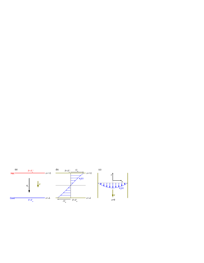
Figure 1: Sketch of the steady states considered in this paper: (a) Fourier flow without ($g=0$) or with ($g\neq 0$) gravity, (b) Couette flow, and (c) force-driven Poiseuille flow.

3 Planar Fourier flow

3.1 Without gravity

In the planar Fourier flow the gas is enclosed between two infinite parallel plates kept at different temperatures [see Fig. 1(a)]. We assume that no external force is acting on the particles ($g=0$) and consider the steady state of the gas with gradients along the direction normal to the plates ($\nabla\to\widehat{\bm{z}}\partial_{z}$) and no flow velocity,

$$\mathbf{u}=\mathbf{0}.$$ (32)

Under these conditions, the Boltzmann equation (6) becomes

$$v_{z}\frac{\partial}{\partial z}f(z,\mathbf{v})=J[\mathbf{v}|f,f]$$ (33)

and the conservation laws of momentum and energy yield

$${P_{zz}}=\text{const},$$ (34)

$$q_{z}=\text{const},$$ (35)

respectively.

In 1979 Asmolov, Makashev, and Nosik AMN79 proved that an exact normal solution of Eq. (33) for Maxwell molecules exists with

$$p=nk_{B}T=\text{const},$$ (36a)

$$T(z)\frac{\partial T(z)}{\partial z}=\text{const}.$$ (36b)

The original paper is rather condensed and difficult to follow, so an independent derivation SBD87 is expounded here.

Since in this problem the only hydrodynamic gradient is the thermal one, i.e., $\partial_{z}T$, the obvious choice of hydrodynamic length is $\ell_{T}=(\partial_{z}\ln T)^{-1}$. As for the mean free path one can take $\ell_{\text{mfp}}=\sqrt{2k_{B}T/m}/\lambda_{11}$. Both quantities are local and their ratio defines the relevant local Knudsen number of the problem, namely

$$\epsilon(z)=\frac{\sqrt{2k_{B}T(z)/m}}{\lambda_{11}(z)}\frac{\partial\ln T(z)}{\partial z}.$$ (37)

Note that $\lambda_{11}(z)\propto n(z)\propto 1/T(z)$, so that $\sqrt{T(z)}\epsilon(z)=\text{const}$, where use has been made of Eqs. (36). Here it is assumed that the separation $2L$ between the plates is large enough as compared with the mean free path to identify a bulk region where the normal solution applies. Such a solution can be nondimensionalized in the form

$$\phi(\mathbf{c};\epsilon)=\frac{1}{n(z)}\left[\frac{2k_{B}T(z)}{m}\right]^{3/2}f(z,\mathbf{v}),$$ (38)

where $\mathbf{c}$ is defined by Eq. (22). All the spatial dependence of $\phi$ is contained in its dependence on $\mathbf{c}$ and $\epsilon$. Thus

$$\frac{\partial f}{\partial z}=\frac{\partial T}{\partial z}\frac{\partial f}{\partial T},$$ (39)

where

$$\frac{\partial f}{\partial T}=n\left(\frac{2k_{B}T}{m}\right)^{-3/2}\left(-\frac{5}{2}T^{-1}\phi+\frac{\partial\mathbf{c}}{\partial T}\cdot\frac{\partial\phi}{\partial\mathbf{c}}+\frac{\partial\epsilon}{\partial T}\frac{\partial\phi}{\partial\epsilon}\right).$$ (40)

Taking into account that $\partial\mathbf{c}/\partial T=-\frac{1}{2}T^{-1}\mathbf{c}$ and $\partial\epsilon/\partial T=-\frac{1}{2}T^{-1}\epsilon$, one finally gets

$$\frac{\partial}{\partial z}f(z,\mathbf{v})=-n\left(\frac{m}{2k_{B}T}\right)^{2}\lambda_{11}\frac{\epsilon}{2}\left(2+\frac{\partial}{\partial\mathbf{c}}\cdot\mathbf{c}+\epsilon\frac{\partial}{\partial\epsilon}\right)\phi(\mathbf{c};\epsilon).$$ (41)

Consequently, the Boltzmann equation (33) becomes

$$-\frac{\epsilon}{2}c_{z}\left(2+\frac{\partial}{\partial\mathbf{c}}\cdot\mathbf{c}+\epsilon\frac{\partial}{\partial\epsilon}\right)\phi(\mathbf{c};\epsilon) = \frac{n}{\lambda_{11}}Q\int d\mathbf{c}_{1}\int d\Omega\,\mathcal{B}(\chi)\left[\phi(\mathbf{c}_{1}^{\prime};\epsilon)\phi(\mathbf{c}^{\prime};\epsilon)-\phi(\mathbf{c}_{1};\epsilon)\phi(\mathbf{c};\epsilon)\right]$$ (42)

$$\equiv \overline{J}[\mathbf{c}|\phi(\epsilon),\phi(\epsilon)].$$

The orthogonal moments of $\phi(\mathbf{c};\epsilon)$ are

$$\mathcal{M}_{k\ell}(\epsilon)=\int d\mathbf{c}\,\psi_{k\ell}(\mathbf{c})\phi(\mathbf{c};\epsilon),$$ (43)

so that

$$\phi(\mathbf{c};\epsilon)=\pi^{-3/2}e^{-c^{2}}\sum_{k=0}^{\infty}\sum_{\ell=0}^{\infty}\mathcal{M}_{k\ell}(\epsilon)\psi_{k\ell}(\mathbf{c}).$$ (44)

Here,

$$\psi_{k\ell}(\mathbf{c})\equiv\psi_{k\ell 0}(\mathbf{c})=N_{k\ell}\sqrt{\frac{2\ell+1}{4\pi}}L_{k}^{(\ell+\frac{1}{2})}(c^{2})c^{\ell}P_{\ell}(c_{z}/c).$$ (45)

The moments $\{\mathcal{M}_{k\ell}\}$ are a subclass of the moments defined by Eq. (24). From the definition of temperature and density, and the fact that the flow velocity vanishes, it follows that

$$\mathcal{M}_{00}=1,\quad\mathcal{M}_{10}=\mathcal{M}_{01}=0.$$ (46)

Taking into account the recurrence relations of the Laguerre and Legendre polynomials AS72 ; GR80 it is easy to prove that

$$\mathbf{c}\cdot\frac{\partial}{\partial\mathbf{c}}\psi_{k\ell}(\mathbf{c})=(2k+\ell)\psi_{k\ell}(\mathbf{c})-2\sqrt{k\left(k+\ell+\frac{1}{2}\right)}\psi_{k-1,\ell}(\mathbf{c}),$$ (47)

$$c_{z}\psi_{k\ell}(\mathbf{c})=\varpi_{k\ell}\psi_{k,\ell+1}(\mathbf{c})-\omega_{k+1,\ell-1}\psi_{k+1,\ell-1}(\mathbf{c})+\varpi_{k,\ell-1}\psi_{k,\ell-1}(\mathbf{c})-\omega_{k\ell}\psi_{k-1,\ell+1}(\mathbf{c}),$$ (48)

where

$$\varpi_{k\ell}\equiv(\ell+1)\left[\frac{k+\ell+\frac{3}{2}}{(2\ell+1)(2\ell+3)}\right]^{1/2},\quad\omega_{k\ell}\equiv(\ell+1)\left[\frac{k}{(2\ell+1)(2\ell+3)}\right]^{1/2}.$$ (49)

Multiplying both sides of Eq. (42) by $\psi_{k\ell}(\mathbf{c})$ and integrating over $\mathbf{c}$ one gets

$$\frac{\epsilon}{2}\left(2k+\ell-1-\epsilon\frac{\partial}{\partial\epsilon}\right)\left(\varpi_{k\ell}\mathcal{M}_{k,\ell+1}-\omega_{k+1,\ell-1}\mathcal{M}_{k+1,\ell-1}+\varpi_{k,\ell-1}\mathcal{M}_{k,\ell-1}-\omega_{k\ell}\mathcal{M}_{k-1,\ell+1}\right)$$ (50)

$$-\epsilon\sqrt{k\left(k+\ell+\frac{1}{2}\right)}\left(\varpi_{k-1,\ell}\mathcal{M}_{k-1,\ell+1}-\omega_{k,\ell-1}\mathcal{M}_{k,\ell-1}+\varpi_{k-1,\ell-1}\mathcal{M}_{k-1,\ell-1}-\omega_{k-1,\ell}\mathcal{M}_{k-2,\ell+1}\right)$$

$$= -\lambdabar_{k\ell}\mathcal{M}_{k\ell}+\frac{1}{\lambda_{11}}\sum_{k^{\prime}\ell^{\prime}k^{\prime\prime}\ell^{\prime\prime}}^{\dagger}C_{k\ell k^{\prime}\ell^{\prime}k^{\prime\prime}\ell^{\prime\prime}}\mathcal{M}_{k^{\prime}\ell^{\prime}}\mathcal{M}_{k^{\prime\prime}\ell^{\prime\prime}}.$$

The choice of the orthogonal moments $\{\mathcal{M}_{k\ell}\}$ simplifies the structure of the collisional terms but, on the other hand, complicates the convective terms. Alternatively, one can use the non-orthogonal moments

$$\overline{M}_{k\ell}(\epsilon)=\int d\mathbf{c}\,c^{2k}c_{z}^{\ell}\phi(\mathbf{c};\epsilon).$$ (51)

In that case, one gets

$$\frac{\epsilon}{2}\left(2k+\ell-1-\epsilon\frac{\partial}{\partial\epsilon}\right)\overline{M}_{k,\ell+1}(\epsilon) = \int d\mathbf{c}\,c^{2k}c_{z}^{\ell}\overline{J}[\mathbf{c}|\phi(\epsilon),\phi(\epsilon)]$$ (52)

$$\equiv \overline{J}_{k\ell}(\epsilon)$$

from Eq. (42). Obviously, $\overline{J}_{k\ell}$ is a bilinear combination of moments $\overline{M}_{k^{\prime}\ell^{\prime}}$ of order equal to or smaller than $\alpha=2k+\ell$.

Equations (50) and (52) reveal the hierarchical character of the moment equations: moments of order $\alpha$ are coupled to moments of lower order but also to moments of order $\alpha+1$. However, the hierarchy can be solved by following a recursive scheme. Of course, the moments of zeroth and first order, as well as one of the two moments of second order are known by definition [cf. Eq. (46)]. The key point is that the moments of order $\alpha\geq 2$ are polynomials in $\epsilon$ of degree $\alpha-2$ and parity $\ell$:

$$\mathcal{M}_{k\ell}(\epsilon)=\sum_{j=0}^{2k+\ell-2}{\mu}_{j}^{(k\ell)}\epsilon^{j},\quad\mu_{j}^{(k\ell)}=0\text{ if }j+\ell=\text{odd},$$ (53)

where $\mu_{j}^{(k\ell)}$ are pure numbers to be determined. Let us see that Eq. (53) is consistent with Eq. (50). First note that all the moments on the left-hand side of Eq. (50) have a parity different from that of $\mathcal{M}_{k\ell}$ but the parity is restored when multiplying by $\epsilon$ or applying the operator $\epsilon^{2}\partial/\partial\epsilon$. Similarly, the condition $2k^{\prime}+\ell^{\prime}+2k^{\prime\prime}+\ell^{\prime\prime}=2k+\ell$ assures that the product $\mathcal{M}_{k^{\prime}\ell^{\prime}}\mathcal{M}_{k^{\prime\prime}\ell^{\prime\prime}}$ is a polynomial of the same degree and parity as those of $\mathcal{M}_{k\ell}$. Next, although the moments $\mathcal{M}_{k,\ell+1}$ and $\mathcal{M}_{k+1,\ell-1}$ are polynomials of degree $2k+\ell-1$, the action of the operator $\epsilon(2k+\ell-1-\epsilon\partial/\partial\epsilon)$ transforms those polynomials into polynomials of degree $2k+\ell-2$.

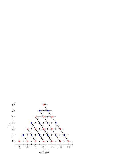
Figure 2: Planar Fourier flow. Sketch of the sequence followed in the recursive determination of the numerical coefficients $\mu_{j}^{(k\ell)}$. All the coefficients of the same order $\alpha=2k+\ell$ are represented by a common circle. The coefficients with $j<\alpha/3$ (represented by circles lying below the dash-dot line) are equal to zero. So are the coefficients with $j<\ell$.

In order to complete the proof that (53) provides a solution to the moment equations (50), a recursive scheme must be devised to get the numerical coefficients $\mu_{j}^{(k\ell)}$. First, notice that the left-hand side of Eq. (50) contains at least the first power of $\epsilon$. So, if $\ell=\text{even}$ one easily gets $\mu_{0}^{(k\ell)}$, provided that $\mu_{0}^{(k^{\prime}\ell^{\prime})}$ is known for $2k^{\prime}+\ell^{\prime}\leq 2k+\ell-2$. Next, if $\ell=\text{odd}$, the coefficient $\mu_{1}^{(k\ell)}$ is determined from the previous knowledge of $\mu_{0}^{(k^{\prime}\ell^{\prime})}$ for $2k^{\prime}+\ell^{\prime}\leq 2k+\ell+1$ and of $\mu_{1}^{(k^{\prime}\ell^{\prime})}$ for $2k^{\prime}+\ell^{\prime}\leq 2k+\ell-2$. Again, if $\ell=\text{even}$ and we know $\mu_{0}^{(k^{\prime}\ell^{\prime})}$ and $\mu_{2}^{(k^{\prime}\ell^{\prime})}$ for $2k^{\prime}+\ell^{\prime}\leq 2k+\ell-2$, as well as $\mu_{1}^{(k^{\prime}\ell^{\prime})}$ for $2k^{\prime}+\ell^{\prime}\leq 2k+\ell+1$, we can get $\mu_{2}^{(k\ell)}$, and so on. As a starting point (moments of zeroth degree) we have $\mathcal{M}_{10}=0$ and $\mathcal{M}_{02}=0$, the latter being a consequence of $\mathcal{M}_{01}=0$. The recursive scheme is sketched in Fig. 2, where the arrows indicate the sequence followed in the determination of $\mu_{j}^{(k\ell)}$. The open (closed) circles represent the coefficients associated with even (odd) $j$ and $\ell$. Notice that the number of coefficients needed to determine a given moment $\mathcal{M}_{k\ell}$ is finite. In fact, the coefficients represented in Fig. 2 are the ones involved in the evaluation of $\mathcal{M}_{k\ell}$ for $k+2\ell\leq 8$. In practice, the number of coefficients actually needed is smaller since

$$\mu_{j}^{(k\ell)}=0\text{ if }j<\text{max}\left(\frac{2k+\ell}{3},\ell\right).$$ (54)

To check the above property, note that Eq. (50) implies that

$$\mu_{j}^{(k\ell)} = \text{L.C.}\left\{\mu_{j-1}^{(k,\ell+1)},\mu_{j-1}^{(k+1,\ell-1)},\mu_{j-1}^{(k-1,\ell+1)},\mu_{j-1}^{(k,\ell-1)},\mu_{j-1}^{(k-2,\ell+1)},\mu_{j-1}^{(k-1,\ell-1)}\right\}$$ (55)

$$+\text{L.C.}\left\{\sum_{j^{\prime}=0}^{j}\mu_{j^{\prime}}^{(k^{\prime}\ell^{\prime})}\mu_{j-j^{\prime}}^{(k^{\prime\prime}\ell^{\prime\prime})}\right\}_{2k^{\prime}+\ell^{\prime}+2k^{\prime\prime}+\ell^{\prime\prime}=2k+\ell,\;|\ell^{\prime}-\ell^{\prime\prime}|\leq\ell\leq\ell^{\prime}+\ell^{\prime\prime}},$$

where L.C. stands for “linear combination of”. If $\mu_{j}^{(k\ell)}=0$ for $j<\frac{1}{3}(2k+\ell)$ then the first term on the right-hand side of Eq. (55) vanishes because $j-1<\frac{1}{3}(2k+\ell-3)<\frac{1}{3}(2k+\ell-1)<\frac{1}{3}(2k+\ell+1)$; the second term also vanishes because either $j^{\prime}<\frac{1}{3}(2k^{\prime}+\ell^{\prime})$ or $j-j^{\prime}<\frac{1}{3}(2k^{\prime\prime}+\ell^{\prime\prime})$. Similarly, if $\mu_{j}^{(k\ell)}=0$ for $j<\ell$ then both terms on the right-hand side vanish because $j-1<\ell-1<\ell+1$ and either $j^{\prime}<\ell^{\prime}$ or $j-j^{\prime}<\ell^{\prime\prime}$, respectively. The property $\mu_{j}^{(k\ell)}=0$ for $j<\ell$ yields

$$\mathcal{M}_{0\ell}=0,\quad\ell\geq 1.$$ (56)

Table 3: Planar Fourier flow. Orthogonal moments $\mathcal{M}_{k\ell}(\epsilon)$ and non-orthogonal moments $\overline{M}_{k\ell}(\epsilon)$ for $2k+\ell\leq 5$ and for $(k,\ell)=(3,1)$, $(4,1)$, and $(5,1)$. In the latter cases the numerical coefficients correspond to the IPL model. Those numerical values are, however, very similar to those corresponding to the VHS and VSS models GTRTS06

$k$	$\ell$	$\mathcal{M}_{k\ell}(\epsilon)$	$\overline{M}_{k\ell}(\epsilon)$
$0$	$0$	$1$	$1$
$0$	$1$	$0$	$0$
$1$	$0$	$0$	$\frac{3}{2}$
$0$	$2$	$0$	$\frac{1}{2}$
$1$	$1$	$\frac{\sqrt{5}}{2}\epsilon$	$-\frac{5}{4}\epsilon$
$0$	$3$	$0$	$-\frac{3}{4}\epsilon$
$2$	$0$	$\frac{7}{2}\sqrt{\frac{5}{6}}\epsilon^{2}$	$\frac{15}{4}+\frac{35}{4}\epsilon^{2}$
$1$	$2$	$-4\sqrt{\frac{2}{21}}\epsilon^{2}$	$\frac{5}{4}+\frac{17}{4}\epsilon^{2}$
$0$	$4$	$0$	$\frac{3}{4}+\frac{81}{28}\epsilon^{2}$
$2$	$1$	$-\frac{17(225-122A_{4}/A_{2})}{18\sqrt{35}(3-2A_{4}/A_{2})}\epsilon^{3}$	$-\frac{35}{4}-\frac{17(225-122A_{4}/A_{2})}{36(3-2A_{4}/A_{2})}\epsilon^{3}$
$1$	$3$	$\sqrt{\frac{3}{5}}\frac{4(100-27A_{4}/A_{2})}{7(11-10A_{4}/A_{2})(3-2A_{4}/A_{2})}\epsilon^{3}$	$-\frac{21}{4}\epsilon-\frac{63225-86656A_{4}/A_{2}+29036(A_{4}/A_{2})^{2}}{84(11-10A_{4}/A_{2})(3-2A_{4}/A_{2})}\epsilon^{3}$
$0$	$5$	$0$	$-\frac{15}{4}\epsilon-\frac{5(3125-2074A_{4}/A_{2})}{84(11-10A_{4}/A_{2})}\epsilon^{3}$
$3$	$1$	$21.86\epsilon^{3}+402.2\epsilon^{5}$	$-\frac{945}{16}\epsilon-726.2\epsilon^{3}-4.371\times 10^{3}\epsilon^{5}$
$4$	$1$	$-9.250\epsilon^{3}-1.471\times 10^{3}\epsilon^{5}-2.816\times 10^{4}\epsilon^{7}$	$-\frac{3465}{8}\epsilon-1.107\times 10^{4}\epsilon^{3}-1.712\times 10^{5}\epsilon^{5}-1.436\times 10^{6}\epsilon^{7}$
$5$	$1$	$2.038\times 10^{3}\epsilon^{5}+1.592\times 10^{5}\epsilon^{7}+3.548\times 10^{6}\epsilon^{9}$	$-\frac{225\,225}{64}\epsilon-\frac{20\,286\,875}{128}\epsilon^{3}-4.593\times 10^{6}\epsilon^{5}-9.292\times 10^{7}\epsilon^{7}-1.031\times 10^{9}\epsilon^{9}$

Since the non-orthogonal moments $\overline{M}_{k\ell}$ are linear combinations of the orthogonal moments $\mathcal{M}_{k^{\prime}\ell^{\prime}}$ with $2k^{\prime}+\ell^{\prime}\leq 2k+\ell$ and $\ell+\ell^{\prime}=\text{even}$, the polynomial form (53) also holds for $\overline{M}_{k\ell}$:

$$\overline{M}_{k\ell}(\epsilon)=\sum_{j=0}^{2k+\ell-2}\overline{m}_{j}^{(k\ell)}\epsilon^{j},\quad\overline{m}_{j}^{(k\ell)}=0\text{ if }j+\ell=\text{odd}.$$ (57)

The explicit expressions for the moments of order smaller than or equal to five are given in Table 3.1. It also includes the moments of order seven, nine, and eleven corresponding to $\ell=1$ and $k=3$, $5$, and $7$, respectively. The result $\mathcal{M}_{02}=0$ or, equivalently, $\overline{M}_{02}=\frac{1}{2}$ imply that

$$P_{zz}=p,$$ (58)

in agreement with Newton’s law (30). The most noteworthy outcome is the linear relationship $\mathcal{M}_{11}(\epsilon)=\frac{\sqrt{5}}{2}\epsilon$ or, equivalently, $\overline{M}_{11}(\epsilon)=-\frac{{5}}{4}\epsilon$. This means that Fourier’s law (31) is exactly verified, i.e.,

$$q_{z}=q_{z}^{\text{NS}},$$ (59)

no matter how large the temperature gradient is. Likewise, $\mathcal{M}_{03}(\epsilon)=0$ or $\overline{M}_{03}(\epsilon)=-\frac{{3}}{4}\epsilon$ imply that

$$\langle v_{z}^{3}\rangle=\frac{3}{5}\langle v^{2}v_{z}\rangle.$$ (60)

The nonlinear character of the solution, however, appears through moments of fourth order and higher. Although those moments are polynomials, the velocity distribution function (44) involves all the powers in the Knudsen number $\epsilon$.

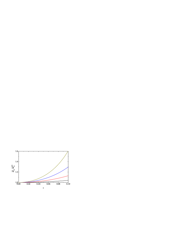
Figure 3: Planar Fourier flow. Plot of the ratio $\overline{M}_{k1}(\epsilon)/\overline{M}_{k1}^{\text{NS}}(\epsilon)$ for, from bottom to top, $k=2$, 3, 4, and 5.

Figure 3 shows the Knudsen number dependence of the moments $\overline{M}_{k1}(\epsilon)$ ($k=2$–$5$) relative to their NS values $\overline{M}_{k1}^{\text{NS}}(\epsilon)=\overline{m}_{1}^{(k1)}\epsilon$. It is quite apparent that, as $\epsilon$ increases, important deviations from the NS predictions exist, even for low values of $k$. This is a consequence of the rapid growth of the nonlinear coefficients of $\mathcal{M}_{k1}(\epsilon)$ and $\overline{M}_{k1}(\epsilon)$ as $k$ increases. This property also holds in the exact solution KDSB89a ; SBG86 ; SBKD89 of the Bhatnagar–Gross–Krook (BGK) model kinetic equation BGK54 ; W54 for the Fourier flow, where it is proven that it is closely related to the divergence of the CE expansion SBKD89 . Whether or not this divergent character of the CE expansion also holds for the solution of the true Boltzmann equation for Maxwell molecules cannot be proven at this stage but it seems sensible to conjecture that the answer is affirmative.

A comparison between the analytical expressions of $\mathcal{M}_{k1}(\epsilon)/\mathcal{M}_{11}(\epsilon)$ for $k=2$–$5$ and the numerical values obtained from the DSMC method for $\epsilon\lesssim 0.08$ shows an excellent agreement GTRTS06 ; GTRTS07 , thus validating both the practical applicability of the theoretical results in the bulk region and the reliability of the simulation method under highly nonequilibrium conditions. Although the validity of Fourier’s law for large thermal gradients is in principle restricted to Maxwell models, it turns out that its practical applicability extends to other potentials, such as that of hard spheres MASG94 .

Before closing this Section, it is worthwhile addressing the spatial dependence of the dimensional moments

$$M_{k\ell}(z) = \int d\mathbf{v}\,v^{2k}v_{z}^{\ell}f(z,\mathbf{v})$$ (61)

$$= n(z)\left[\frac{2k_{B}T(z)}{m}\right]^{k+\ell/2}\overline{M}_{k\ell}(\epsilon(z)).$$

Taking into account Eq. (57) and the fact that $\sqrt{T(z)}\epsilon(z)=\sqrt{T_{0}}\epsilon_{0}=\text{const}$ (where $T_{0}$ and $\epsilon_{0}$ are the temperature and the Knudsen number evaluated at $z=0$, respectively), one can easily get

$$M_{k\ell}(z)=\frac{2p}{m}\left(\epsilon_{0}^{2}\frac{2k_{B}T_{0}}{m}\right)^{k+\ell/2-1}\sum_{j=0}^{k-1+[\ell/2]}\overline{m}_{2k+\ell-2-2j}^{(k\ell)}\left[\frac{T(z)}{\epsilon_{0}^{2}T_{0}}\right]^{j},$$ (62)

where $[\ell/2]$ is the integer part of $\ell/2$ and it is understood that $2k+\ell\geq 2$. Equation (62) shows that $M_{k\ell}(z)$ is just a polynomial in $T(z)$ of degree $k-1+[\ell/2]$. As for the spatial dependence of temperature, Eq. (36b) implies that

$$T(z)=T_{0}\sqrt{1+\frac{2\epsilon_{0}}{\ell_{\text{mfp}}(0)}z},$$ (63)

where $\ell_{\text{mfp}}(0)\propto T_{0}^{3/2}/p$ is the local mean free path at $z=0$. It is convenient to define a scaled spatial variable $s$ as

$$s=\int_{0}^{z}dz^{\prime}\,\lambda_{11}(z^{\prime}).$$ (64)

Since $\lambda_{11}(z)\propto p/T(z)$, one has

$$s=\frac{\sqrt{2k_{B}T_{0}/m}}{\epsilon_{0}}\left[\sqrt{1+\frac{2\epsilon_{0}}{\ell_{\text{mfp}}(0)}z}-1\right].$$ (65)

In terms of this new variable the temperature profile (63) becomes linear,

$$T(s)=T_{0}\left(1+\frac{\epsilon_{0}}{\sqrt{2k_{B}T_{0}/m}}s\right).$$ (66)

Likewise, according to Eq. (62), the moment $M_{k\ell}(s)$ is a polynomial in $s$ of degree $k-1+[\ell/2]$. The exact solution of the BGK model for any interaction potential KDSB89a ; SBG86 ; SBKD89 keeps the linear and polynomial forms of $T(s)$ and $M_{k\ell}(s)$, respectively, as functions of $s$. The only influence of the potential appears through the temperature dependence of the collision frequency (which plays the role of $\lambda_{11}$), so that when applying Eq. (64) one does not get Eqs. (63) and (65), except for Maxwell molecules. The solution of the Boltzmann equation for Maxwell molecules described here can be extended to the case of gaseous mixtures N81 .

3.2 With gravity

Let us suppose that the planar Fourier flow is perturbed by a constant body force $\mathbf{F}=-mg\widehat{\mathbf{z}}$ orthogonal to the plates and directed downwards (e.g., gravity). This situation is sketched in Fig. 1(a) with $g\neq 0$ and has the same geometry as the Rayleigh–Bénard problem. In fact, we can define a microscopic local Rayleigh number as

$$\gamma\equiv\frac{g}{\lambda_{11}^{2}}\frac{\partial\ln T}{\partial z}=\frac{g\epsilon}{\lambda_{11}\sqrt{2k_{B}T/m}},$$ (67)

where in the last step use has been made of Eq. (37). The dimensionless parameters $\gamma$ and $\epsilon$ characterize the normal state of the system. Note that $\gamma=0$ implies that either $g=0$ but $\epsilon\neq 0$ (Fourier flow without gravity) or $\epsilon=0$ but $g\neq 0$ (equilibrium state with a pressure profile given by the barometric formula).

The conventional Rayleigh number is $\text{Ra}\sim|\gamma|\left({L}/{\ell_{\text{mfp}}}\right)^{4}$. The situation depicted in Fig. 1(a) corresponds to a gas heated from above ($\partial_{z}T>0\Rightarrow\gamma>0$). If the gas is heated from below then $\partial_{z}T<0$ and $\gamma<0$. We assume that either $\gamma>0$ or $\gamma<0$ but $\text{Ra}\lesssim 1700$, so that the gas at rest is stable and there is no convection ($\mathbf{u}=\mathbf{0}$). On the other hand, rarefied gases can present a Rayleigh–Bénard instability under appropriate conditions CS92 ; SAS97 .

The stationary Boltzmann equation for the problem at hand reads

$$v_{z}\frac{\partial}{\partial z}f(z,\mathbf{v})-g\frac{\partial}{\partial v_{z}}f(z,\mathbf{v})=J[\mathbf{v}|f,f].$$ (68)

In this case the moment hierarchy (16) becomes

$$\frac{\partial}{\partial z}M_{k,\ell+1}(z)+g\left[2kM_{k-1,\ell+1}(z)+\ell M_{k,\ell-1}(z)\right]=J_{k\ell}(z),$$ (69)

where the moments $M_{k\ell}$ are defined by the first equality of Eq. (61) and $J_{k\ell}$ are the corresponding collisional moments. In particular, conservation of momentum and energy imply that $\partial_{z}M_{02}=-gn$ and $\partial_{z}M_{11}=0$, respectively. In other words, one has

$$\frac{\partial P_{zz}(z)}{\partial z}=-g\rho(z),$$ (70)

where $\rho=mn$ is the mass density, plus Eq. (35). The presence of the terms proportional to $g$ in Eqs. (68) and (69) complicates the problem significantly, thus preventing an exact solution (for general $\epsilon$ and $\gamma$), even in the case of Maxwell molecules. On the other hand, if $|\gamma|\ll 1$ one can treat it as a small parameter and carry out a perturbation expansion of the form

$$f(z,\mathbf{v})=f^{(0)}(z,\mathbf{v})+f^{(1)}(z,\mathbf{v})\gamma+f^{(2)}(z,\mathbf{v})\gamma^{2}+\cdots,$$ (71)

$$M_{k\ell}(z)=M_{k\ell}^{(0)}(z)+M_{k\ell}^{(1)}(z)\gamma+M_{k\ell}^{(2)}(z)\gamma^{2}+\cdots.$$ (72)

Here the superscript $(0)$ denotes the reference state without gravity, i.e., the one analyzed in Sec. 3.1. When the expansion (72) is inserted into Eq. (69) one gets a recursive scheme allowing one to obtain, in principle, $\{M_{k\ell}^{(j+1)}\}$ from the previous knowledge of $\{M_{k\ell}^{(j)}\}$. The technical details can be found in Ref. TGS97 and here only the relevant final results will be presented. First, it turns out that the temperature field $T^{(j)}$ of order $\gamma^{j}$ is a polynomial of degree $j+1$ in the scaled variable $s$ defined by Eq. (64). This generalizes the linear relationship (66) found for $T^{(0)}$ (i.e., in the absence of gravity). Analogously, $M_{k\ell}^{(j)}$ for $2k+\ell\geq 2$ is a polynomial in $s$ of degree $k+j-1+[\ell/2]$. In order to fully determine $M_{k\ell}^{(j)}$ it is necessary to make use of the collisional moments $J_{k^{\prime}\ell^{\prime}}$ with $2k^{\prime}+\ell^{\prime}\leq 2(2k+\ell+j-1)$. The main results are TGS97

$$\frac{\partial}{\partial z}T\frac{\partial T}{\partial z}=-\frac{104}{5}\frac{m\lambda_{11}^{2}T}{k_{B}}\gamma^{2}+\mathcal{O}(\gamma^{3}),$$ (73)

$$\frac{P_{zz}-p}{p}=\frac{128}{45}\gamma^{2}+\mathcal{O}(\gamma^{3}),$$ (74)

$$q_{z}=q_{z}^{\text{NS}}\left[1+\frac{46}{5}\gamma+\mathcal{O}(\gamma^{2})\right],$$ (75)

$${\langle v_{z}^{3}\rangle}=\frac{3}{5}{\langle v^{2}v_{z}\rangle}\left[1+\frac{64}{105}\gamma+\mathcal{O}(\gamma^{2})\right].$$ (76)

Equations (73)–(76) account for the first corrections to Eqs. (36b), (58), (59), and (60), respectively, due to the presence of gravity. In addition, given Eqs. (70) and (74), one has ${\partial_{z}p}=-\rho g+\mathcal{O}(\gamma^{3})$. According to Eq. (75) the presence of gravity produces an enhancement of the heat flux with respect to its NS value when heating from above ($\gamma>0$). The opposite effect occurs when heating from below ($\gamma<0$).

The above theoretical predictions for Maxwell molecules were seen to agree at a semi-quantitative level with DSMC results for hard spheres TTS00 . Moreover, an analysis similar to that of Ref. TGS97 can be carried out from the BGK kinetic model. The results though order $\gamma^{6}$ TGS99 strongly suggest the asymptotic character of the series (71) and (72). The theoretical asymptotic analysis of Ref. TGS99 agrees well with a finite-difference numerical solution of the BGK equation DST99 .

4 Planar Couette flow

Apart from the Fourier flow, the steady planar Couette flow is perhaps the most basic nonequilibrium state. It corresponds to a fluid enclosed between two infinite parallel plates maintained in relative motion [see Fig. 1(b)]. The plates can be kept at the same temperature or, more generally, at two different temperatures. In either case, in addition to a velocity profile $\mathbf{u}=u_{x}(z)\widehat{\mathbf{x}}$, a temperature profile $T(z)$ appears in the system to produce the non-uniform heat flux compensating for the viscous heating. As a consequence, there are two main hydrodynamic lengths: the one associated with the thermal gradient (as in the Fourier flow), i.e., $\ell_{T}=(\partial_{z}\ln T)^{-1}$, plus the one associated with the shear rate, namely $\ell_{u}=\sqrt{2k_{B}T/m}(\partial u_{x}/\partial z)^{-1}$. Therefore, two independent (local) Knudsen numbers can be defined: the reduced thermal gradient defined by Eq. (37) and the reduced shear rate

$$a=\frac{1}{\lambda_{02}}\frac{\partial u_{x}}{\partial z},$$ (77)

where for convenience here we use the collision frequency $\lambda_{02}$ associated with the viscosity, while in Eq. (37) use is made of the collision frequency $\lambda_{11}$ associated with the thermal conductivity. Like in the planar Fourier flow, the Boltzmann equation of the problem reduces to Eq. (33). The conservation of momentum implies Eq. (34) as well as

$$P_{xz}=\text{const}.$$ (78)

However, in contrast to Eq.  (35), now the energy conservation equation becomes

$$\frac{\partial q_{z}}{\partial z}+P_{xz}\frac{\partial u_{x}}{\partial z}=0.$$ (79)

In 1981, Makashev and Nosik MN81 ; N83 extended to the planar Couette flow the solution found in Ref. AMN79 for the planar Fourier flow. More specifically, they proved that a normal solution to Eq. (33) for Maxwell molecules exists characterized by a constant pressure, i.e., Eq. (36a), and velocity and temperature profiles satisfying

$$T(z)\frac{\partial{u}_{x}(z)}{\partial z}=\text{const},$$ (80a)

$$T(z)\frac{\partial}{\partial z}T(z)\frac{\partial T(z)}{\partial z}=\text{const}.$$ (80b)

These two equations are the counterparts to Eqs. (32) and (36b), respectively. Since $\lambda_{02}\propto p/T$, Eq. (80a) implies that the dimensionless local shear rate defined by Eq. (77) is actually uniform across the system, i.e.,

$$a=\text{const}.$$ (81)

In the NS description, Eq. (81) follows immediately from the constitutive equation (30) and the exact conservation laws (34) and (78). Here, however, Eq. (81) holds even when both Knudsen numbers $\epsilon$ and $a$ are not small and Newton’s law (30) fails. This failure can be characterized by means of a nonlinear (dimensionless) shear viscosity $\eta^{*}(a)$ and two (dimensionless) normal stress differences $\Delta_{1,2}(a)$ defined by

$$P_{xz}=-\eta^{*}(a)\eta_{\text{NS}}\frac{\partial u_{x}}{\partial z},$$ (82)

$$\frac{P_{xx}-P_{zz}}{p}={\Delta_{1}(a)},\quad\frac{P_{yy}-P_{zz}}{p}={\Delta_{2}(a)}.$$ (83)

Note that Eqs. (34), (36a), (78), and (81) are consistent with Eqs. (82) and (83), even though $\eta^{*}(a)\neq 1$ and $\Delta_{1,2}(a)\neq 0$.

As for Eq. (80b), it can also be justified at the NS level by the constitutive equation (31) and the exact conservation equation (79). Again, the validity of Eq. (80b) goes beyond the scope of Fourier’s law (31). More specifically, Eq. (79) yields

$$\frac{1}{\lambda_{11}}\frac{\partial q_{z}}{\partial z}=\frac{3p}{2}\eta^{*}(a)a^{2}=\text{const}.$$ (84)

Equations (80b) and (84) are consistent with a heat flux component $q_{z}$ given by a modified Fourier’s law of the form

$$q_{z}=-\kappa^{*}(a)\kappa_{\text{NS}}\frac{\partial T}{\partial z},$$ (85)

where $\kappa^{*}(a)\neq 1$ is a nonlinear (dimensionless) thermal conductivity. Equations (84) and (85) allow us to identify the constant on the right-hand side of Eq. (80b), namely

$$T\frac{\partial}{\partial z}T\frac{\partial T}{\partial z}=-\frac{3m(\lambda_{11}T)^{2}}{5k_{B}}a^{2}\theta(a)=\text{const},$$ (86)

where $\theta(a)\equiv\eta^{*}(a)/\kappa^{*}(a)$ is a sort of nonlinear Prandtl number. Making use of Eq. (37), Eq. (86) can be rewritten as

$$\sqrt{T}\epsilon\frac{\partial}{\partial T}\left(\sqrt{T}\epsilon\right)=-\frac{6}{5}a^{2}\theta(a).$$ (87)

To prove the consistency of the assumed hydrodynamic profiles (36a) and (80) we can proceed along similar lines as in the case of the planar Fourier flow GS03 ; TS95 . First, we introduce the dimensionless velocity distribution function

$$\phi(\mathbf{c};\epsilon,a)=\frac{1}{n(z)}\left[\frac{2k_{B}T(z)}{m}\right]^{3/2}f(z,\mathbf{v}),$$ (88)

where now it is important to notice that the definition (22) includes the flow velocity $\mathbf{u}$. Therefore,

$$\frac{\partial f}{\partial z}=\frac{\partial T}{\partial z}\frac{\partial f}{\partial T}+\frac{\partial u_{x}}{\partial z}\frac{\partial f}{\partial u_{x}},$$ (89)

where

$$\frac{\partial f}{\partial u_{x}}=-n\left(\frac{m}{2k_{B}T}\right)^{2}\frac{\partial\phi}{\partial c_{x}}.$$ (90)

The derivative $\partial f/\partial T$ is given again by Eq. (40), but now $\partial\epsilon/\partial T=-T^{-1}\left(\frac{1}{2}\epsilon+\frac{6}{5}\epsilon^{-1}a^{2}\theta\right)$ on account of Eq. (87). In summary,

$$\frac{\partial}{\partial z}f(z,\mathbf{v})=-n\left(\frac{m}{2k_{B}T}\right)^{2}\lambda_{11}\left[\frac{\epsilon}{2}\left(2+\frac{\partial}{\partial\mathbf{c}}\cdot\mathbf{c}+\epsilon\frac{\partial}{\partial\epsilon}\right)+\frac{6}{5}a^{2}\theta(a)\frac{\partial}{\partial\epsilon}+\frac{3}{2}a\frac{\partial}{\partial c_{x}}\right]\phi(\mathbf{c};\epsilon,a).$$ (91)

Consequently, the Boltzmann equation (33) becomes

$$-c_{z}\left[\frac{\epsilon}{2}\left(2+\frac{\partial}{\partial\mathbf{c}}\cdot\mathbf{c}+\epsilon\frac{\partial}{\partial\epsilon}\right)\right. + \left.\frac{6}{5}a^{2}\theta(a)\frac{\partial}{\partial\epsilon}+\frac{3}{2}a\frac{\partial}{\partial c_{x}}\right]\phi(\mathbf{c};\epsilon,a)$$ (92)

$$= \frac{n}{\lambda_{11}}Q\int d\mathbf{c}_{1}\int d\Omega\,\mathcal{B}(\chi)\left[\phi(\mathbf{c}_{1}^{\prime};\epsilon,a)\phi(\mathbf{c}^{\prime};\epsilon,a)-\phi(\mathbf{c}_{1};\epsilon,a)\phi(\mathbf{c};\epsilon,a)\right]$$

$$\equiv \overline{J}[\mathbf{c}|\phi(\epsilon,a),\phi(\epsilon,a)].$$

Of course, Eq. (92) reduces to Eq. (42) in the special case of the Fourier flow ($a=0$).

For simplicity, we consider now the following non-orthogonal moments of order $\alpha=2k+\ell$,

$$\overline{M}_{k\ell{h}}(\epsilon,{a})=\int d\mathbf{c}\,c^{2k}c_{z}^{\ell{-h}}{c_{x}^{h}}\phi(\mathbf{c};\epsilon,{a}),\quad 0\leq h\leq\ell,$$ (93)

instead of the orthogonal moments (24). By definition, $\overline{M}_{000}=1$, $\overline{M}_{010}=\overline{M}_{011}=0$, and $\overline{M}_{100}=\frac{3}{2}$. According to Eq. (92) the moment equations read

$$\left[\frac{\epsilon}{2}\left(2k+\ell-1-\epsilon\frac{\partial}{\partial\epsilon}\right)\right. - \left.\frac{6}{5}a^{2}\theta(a)\frac{\partial}{\partial\epsilon}\right]\overline{M}_{k,\ell+1,{h}}+\frac{3}{2}a\left(2k\overline{M}_{k-1,\ell+2,h+1}+h\overline{M}_{k,\ell,h-1}\right)$$ (94)

$$= \int d\mathbf{c}\,c^{2k}c_{z}^{\ell{-h}}{c_{x}^{h}}\overline{J}[\mathbf{c}|\phi,\phi]\equiv\overline{J}_{k\ell{h}}(\epsilon,{a}).$$

While this hierarchy is much more involved than Eq. (52), it can be easily checked to be consistent with solutions of the form

$$\overline{M}_{k\ell h}(\epsilon,a)=\sum_{j=0}^{2k+\ell-2}\overline{m}_{j}^{(k\ell h)}(a)\epsilon^{j},\quad\overline{m}_{j}^{(k\ell h)}(a)=0\text{ if }j+\ell=\text{odd}.$$ (95)

Therefore, the moments $\overline{M}_{k\ell{h}}(\epsilon,{a})$ of order $2k+\ell\geq 2$ are again polynomials in the thermal Knudsen number $\epsilon$ of degree $2k+\ell-2$ and parity $\ell$. In particular, the moments of second order are independent of $\epsilon$, which yields Eqs. (82) and (83) with

$$\eta^{*}(a)=-\frac{2\overline{m}_{0}^{(021)}(a)}{a},$$ (96)

$$\Delta_{1}(a)=2\left[\overline{m}_{0}^{(022)}(a)-\overline{m}_{0}^{(020)}(a)\right],\quad\Delta_{2}(a)=3-2\left[\overline{m}_{0}^{(022)}(a)+2\overline{m}_{0}^{(020)}(a)\right].$$ (97)

The third-order moments are linear in $\epsilon$, as anticipated by Eq. (85) with

$$\kappa^{*}(a)=-\frac{4}{5}\overline{m}_{1}^{(110)}(a).$$ (98)

Besides, the shearing induces a component of the heat flux parallel to the flow but normal to the thermal gradient:

$$q_{x}=\Phi(a)\kappa_{\text{NS}}\frac{\partial T}{\partial z},\quad\Phi(a)=\frac{4}{5}\overline{m}_{1}^{(111)}(a).$$ (99)

Since the reduced shear rate $a$ is constant in the bulk domain, it is not difficult to get the spatial dependence of the dimensional moments

$$M_{k\ell h}(z) = \int d\mathbf{v}\,|\mathbf{v}-\mathbf{u}(z)|^{2k}v_{z}^{\ell-h}[v_{x}-u_{x}(z)]^{h}f(z,\mathbf{v})$$ (100)

$$= n(z)\left[\frac{2k_{B}T(z)}{m}\right]^{k+\ell/2}\overline{M}_{k\ell h}(\epsilon(z),a).$$

Inserting Eq. (95) into Eq. (100) one has

$$M_{k\ell h}(z)=\frac{2p}{m}\left(\frac{2k_{B}}{m}\right)^{k+\ell/2-1}\;\sum_{j=0}^{k-1+[\ell/2]}\overline{m}_{2k+\ell-2-2j}^{(k\ell h)}(a)\left[\sqrt{T(z)}\epsilon(z)\right]^{2k+\ell-2-2j}\left[T(z)\right]^{j}.$$ (101)

As in the case of the Fourier flow, it is convenient to introduce the scaled spatial variable $s$ through Eq. (64). In terms of this variable, Eqs. (80) can be integrated to give

$$u_{x}(s)=\frac{3}{2}as,\quad T(s)=T_{0}\left[1+\frac{\epsilon_{0}}{\sqrt{2k_{B}T_{0}/m}}s-\frac{3m}{10k_{B}T_{0}}a^{2}\theta(a)s^{2}\right],$$ (102)

where use has been made of Eqs. (77) and (86). Thus, $u_{x}$ and $T$ are linear and quadratic functions of $s$, respectively. Analogously, $\sqrt{T}\epsilon$ is linear in $s$, namely

$$\sqrt{T(s)}\epsilon(s)=\sqrt{T_{0}}\epsilon_{0}-\frac{3\sqrt{2m/k_{B}}}{5}a^{2}\theta(a)s.$$ (103)

Therefore, in view of Eq. (101), it turns out that, if expressed in terms of $s$, the dimensional moment $M_{k\ell h}(s)$ is a polynomial of degree $2k+\ell-2$. Inverting Eq. (64) one gets the relationship between $s$ and $z$:

$$z=\ell_{\text{mfp}}(0)\frac{s}{\sqrt{2k_{B}T_{0}/m}}\left[1+\frac{\epsilon_{0}}{2}\frac{s}{\sqrt{2k_{B}T_{0}/m}}-a^{2}\theta(a)\frac{s^{2}}{10k_{B}T_{0}/m}\right].$$ (104)

The solution to this cubic equation gives $s$ as a function of $z$. Of course, Eqs. (65) and (66) are recovered from Eqs. (104) and (102), respectively, by setting $a=0$.

The key difference with respect to the Fourier flow case [cf. Eq. (57)] is that, while the coefficients $\overline{m}_{j}^{(k\ell)}$ were pure numbers, now the coefficients $\overline{m}_{j}^{(k\ell h)}(a)$, as well as $\theta(a)$, are nonlinear functions of the shear Knudsen number $a$ (of parity equal to $h$). Unfortunately, the full dependence $\overline{m}_{j}^{(k\ell h)}(a)$ cannot be recursively obtained from Eq. (94) because the term headed by $a^{2}\theta(a)$ couples $\overline{m}_{j}^{(k\ell h)}(a)$ to $\overline{m}_{j+1}^{(k,\ell+1,h)}(a)$. On the other hand, since that coupling is at least of order $a^{2}$, it is possible to get recursively the numerical coefficients of the expansions of $\overline{m}_{j}^{(k\ell h)}(a)$ in powers of $a$ TS95 :

$$\overline{m}_{j}^{(k\ell h)}(a)=\sum_{i=0}^{\infty}\overline{m}_{ji}^{(k\ell h)}a^{i},\quad\overline{m}_{ji}^{(k\ell h)}=0\text{ if }i+h=\text{odd}.$$ (105)

Obviously, the coefficients $\overline{m}_{j0}^{(k\ell h)}$ are those of the Fourier flow and are obtained from the scheme of Fig. 2. Their knowledge allows one to get $\overline{m}_{j1}^{(k\ell h)}$, and so on. In general, the coefficients $\overline{m}_{ji}^{(k\ell h)}$ can be determined from the previous knowledge of the coefficients $\overline{m}_{j^{\prime}i^{\prime}}^{(k^{\prime}\ell^{\prime}h^{\prime})}$ with $2k^{\prime}+\ell^{\prime}\leq 2k+\ell$ and $2k^{\prime}+\ell^{\prime}+j^{\prime}+i^{\prime}\leq 2k+\ell+j+i$. From the results to order $a^{3}$ one gets GS03 ; TS95

$$\eta^{*}(a)=1+\eta_{2}^{*}a^{2}+\mathcal{O}(a^{4}),\quad\eta_{2}^{*}=-\frac{149}{45},$$ (106)

$$\kappa^{*}(a)=1+\kappa_{2}^{*}a^{2}+\mathcal{O}(a^{4}),\quad\kappa_{2}^{*}=-\frac{15238+45A_{4}/A_{2}}{2100},$$ (107)

$$\theta(a)=1+\theta_{2}a^{2}+\mathcal{O}(a^{4}),\quad\theta_{2}=\frac{24854+135A_{4}/A_{2}}{6300},$$ (108)

$$\Delta_{1}(a)=\frac{14}{5}a^{2}+\mathcal{O}(a^{4}),\quad\Delta_{2}(a)=\frac{4}{5}a^{2}+\mathcal{O}(a^{4}),$$ (109)

$$\Phi(a)=\frac{7}{2}a+\mathcal{O}(a^{3}).$$ (110)

The coefficients in Eqs. (109) and (110) are of Burnett order, while those in Eqs. (106)–(108) are of super-Burnett order. Table 4 compares the latter coefficients with the predictions of the BGK kinetic model BSD87 ; D90 ; GS03 ; KDSB89b , the Ellipsoidal Statistical (ES) kinetic model GH97 ; MG98 first proposed by Holway ATPP00 ; C88 ; H66 , Grad’s 13-moment method RC97 ; RC98 , and the regularized 13-moment (R13) method S05 ; ST08 ; TTS09 . Despite their simplicity, the BGK and ES kinetic models provide reasonable values. The 13-moment method, however, gives wrong signs for $\kappa_{2}^{*}$ and $\theta_{2}$. On the other hand, the more elaborate R13-moment method practically predicts the right results.

Table 4: Planar Couette flow. Numerical values of the super-Burnett coefficients $\eta_{2}^{*}$, $\kappa_{2}^{*}$, and $\theta_{2}=\eta_{2}^{*}-\kappa_{2}^{*}$, according to the Boltzmann equation (for the IPL Maxwell potential) and several approximations

Coefficient	Boltzmann	BGK model	Ellipsoidal Statistical model	13-moment	R13-moment
$\eta_{2}^{*}$	$-3.311$	$-3.60$	$-4.20$	$-2.60$	$-3.311$
$\kappa_{2}^{*}$	$-7.260$	$-6.48$	$-7.88$	$0.42$	$-7.256$
$\theta_{2}$	$3.948$	$2.88$	$3.68$	$-3.02$	$3.945$

The quantities (82), (83), (85), and (99) correspond to moments of second and third order. As an illustration of higher-order moments, let us introduce the quantities

$$R_{k}(\epsilon) \equiv \lim_{a\to 0}\frac{\overline{M}_{k21}(\epsilon,a)}{\overline{M}_{021}(a)}=\lim_{a\to 0}\frac{\langle c^{2k}c_{x}c_{z}\rangle}{\langle c_{x}c_{z}\rangle}$$ (111)

$$= \frac{1}{\overline{m}_{01}^{(021)}}\sum_{j=0}^{k}{\overline{m}_{2j,1}^{(k21)}}\epsilon^{2j}.$$

The functions $R_{k}(\epsilon)$ for $k=1$, 2, and 3 are listed in Table 4, while Fig. 4 shows the ratio $R_{k}(\epsilon)/R_{k}^{\text{NS}}$, where $R_{k}^{\text{NS}}=R_{k}(0)$ is the NS value.

Table 5: Planar Couette flow. Scaled moments $R_{k}(\epsilon)$, as defined by Eq. (111), for $k=1$, 2, and 3

$k$	$R_{k}(\epsilon)$
$1$	$\frac{7}{2}+22.41\epsilon^{2}$
$2$	$\frac{63}{4}+339.8\epsilon^{2}+2.184\times 10^{3}\epsilon^{4}$
$3$	$\frac{693}{8}+4.167\times 10^{3}\epsilon^{2}+7.153\times 10^{4}\epsilon^{4}+5.977\times 10^{5}\epsilon^{6}$

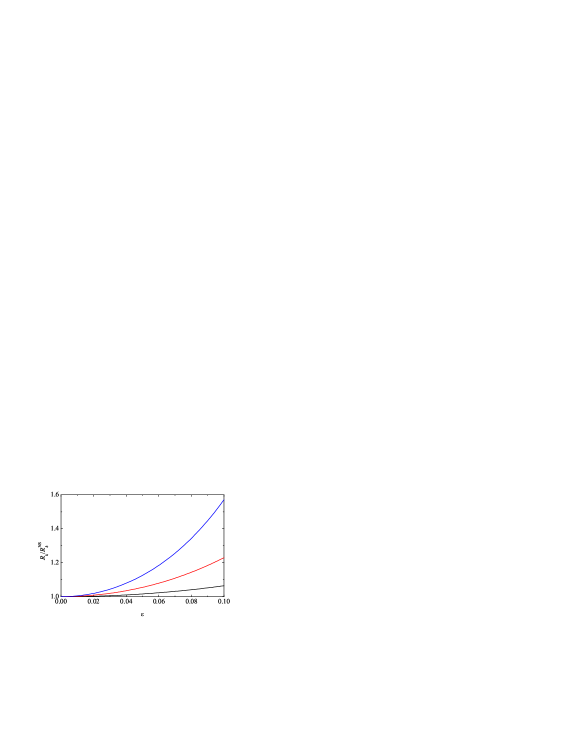
Figure 4: Planar Couette flow. Plot of the ratio $R_{k}(\epsilon)/R_{k}^{\text{NS}}$ for, from bottom to top, $k=1$, 2, and 3.

Analogously to the case of the Fourier flow, a comparison between the theoretical expressions of the orthogonal moments related to $R_{k}(\epsilon)$ for $k=1$–$3$ and the numerical values obtained from the DSMC method for $\epsilon\lesssim 0.08$ presents an excellent agreement GTRTS06 ; GTRTS07 . Although the full dependence of the moments on the reduced shear rate $a$ cannot be evaluated exactly from the Boltzmann equation, this goal has been achieved in the case of the BGK BSD87 ; GS03 ; KDSB89b and ES GH97 ; GS03 kinetic models, where one can also obtain the velocity distribution function $\phi(\mathbf{c};\epsilon,a)$ itself. The results show that the CE expansion of the distribution function in powers of both $\epsilon$ and $a$ is only asymptotic. The BGK and ES predictions for the coefficients $\eta^{*}(a)$, $\kappa^{*}(a)$, $\theta(a)$, $\Delta_{1,2}(a)$, and $\Phi(a)$ compare favorably well with DSMC results for both Maxwell molecules and hard spheres MSG00 . The BGK kinetic model has also been used to assess the influence of an external body force $\mathbf{F}=-mg\widehat{\mathbf{z}}$ on the transport properties of the Couette flow TGS99b . The results show that such an influence tends to decrease as the shear rate increases in the case of the rheological properties $\eta^{*}(a)$ and $\Delta_{1,2}(a)$, while it is especially important in the case of the heat flux coefficient $\Phi(a)$.

5 Force-driven Poiseuille flow

One of the most well-known textbook examples in fluid dynamics is the Poiseuille flow T88 . It consists of the steady flow along a channel of constant cross section produced by a pressure difference at the distant ends of the channel. At least at the NS order, essentially the same type of flow can be generated by the action of a uniform longitudinal body force $\mathbf{F}=-mg\widehat{\mathbf{z}}$ (e.g., gravity) instead of a longitudinal pressure gradient. This force-driven Poiseuille flow [see Fig. 1(c)] has received much attention from computational KMZ87 ; KMZ89 ; MBG97 ; RC98b ; TE97 ; TTE97 ; ZGA02 and theoretical AS92 ; ATN02 ; ELM94 ; GVU08 ; HM99 ; RC98b ; STS03 ; ST06 ; ST08 ; TTS09 ; TSS98 ; TS94 ; TS01 ; TS04 ; UG99b ; X03 points of view. This interest has been mainly fueled by the fact that the force-driven Poiseuille flow provides a nice example illustrating the limitations of the NS description in the bulk domain (i.e., far away from the boundary layers).

The Boltzmann equation for this problem becomes

$$v_{x}\frac{\partial}{\partial x}f(x,\mathbf{v})-g\frac{\partial}{\partial v_{z}}f(x,\mathbf{v})=J[\mathbf{v}|f,f].$$ (112)

The apparent similarity to Eq. (68) is deceptive: although the velocity distribution function only depends on the coordinate ($x$) orthogonal to the plates, this axis is perpendicular to the force, in contrast to the case of Eq. (68). The conservation laws of momentum and energy imply

$${P_{xx}}=\text{const},\quad\frac{\partial P_{xz}}{\partial x}=-\rho g,\quad\frac{\partial q_{x}}{\partial x}+P_{xz}\frac{\partial u_{z}}{\partial x}=0.$$ (113)

The appropriate (dimensional) moments are defined similarly to the first line of Eq. (100), namely

$$M_{k\ell h}(x)=\int d\mathbf{v}\,|\mathbf{v}-\mathbf{u}(x)|^{2k}v_{x}^{\ell-h}[v_{z}-u_{z}(x)]^{h}f(x,\mathbf{v}),\quad 0\leq h\leq\ell.$$ (114)

Because of the symmetry properties of the problem, $u_{z}(x)$ is an even function of $x$ and $M_{k\ell h}(x)$ is an even (odd) function of $x$ if $\ell-h$ is even (odd). Seen as functions of $g$, $u_{z}(x)-u_{z}(0)$ is an odd function, while $M_{k\ell h}(x)$ is an even (odd) function if $h$ is even (odd). The corresponding hierarchy of moment equations reads

$$\frac{\partial}{\partial x}M_{k,\ell+1,h}(x) + \frac{\partial u_{z}(x)}{\partial x}\left[2kM_{k-1,\ell+2,h+1}(x)+hM_{k,\ell,h-1}(x)\right]$$ (115)

$$+ g\left[2kM_{k-1,\ell+1,h+1}(x)+hM_{k,\ell-1,h-1}(x)\right]=J_{k\ell h}(x).$$

Again, moments of order $2k+\ell$ are coupled to moments of order $2k+\ell+1$, and so their full dependence on $x$ and $g$ cannot be determined, even in the bulk domain and for Maxwell models. However, the problem can be solved by a recursive scheme TSS98 if the moments are expanded in powers of $g$ around a reference equilibrium state parameterized by $u_{z}(0)=u_{0}$, $p(0)=p_{0}$, and $T(0)=T_{0}$:

$$u_{z}(x)=u_{0}+u_{z}^{(1)}(x)g+u_{z}^{(3)}(x)g^{3}+\cdots,\quad p(x)=p_{0}+p^{(2)}(x)g^{2}+p^{(4)}(x)g^{4}+\cdots,$$ (116)

$$T(x)=T_{0}+T^{(2)}(x)g^{2}+T^{(4)}(x)g^{4}+\cdots,\quad M_{k\ell h}(x)=M_{k\ell h}^{(0)}+M_{k\ell h}^{(1)}g+M_{k\ell h}^{(2)}g^{2}+\cdots.$$ (117)

Due to symmetry reasons, $u_{z}^{(j)}(x)=0$ if $j=\text{even}$, $p^{(j)}(x)=T^{(j)}(x)=0$ if $j=\text{odd}$, and $M_{k\ell h}^{(j)}(x)=0$ if $h+j=\text{odd}$. The functions $u_{z}^{(j)}(x)$, $p^{(j)}(x)$, and $T^{(j)}(x)$ are even, while $M_{k\ell h}^{(j)}(x)$ has the same parity as $\ell-h$. In fact, it turns out that those functions are just polynomials of degree $2j$ (or $2j-1$ if $\ell-h=\text{odd}$) TSS98 , namely

$$u_{z}^{(j)}(x)=\sum_{i=1}^{j}u_{z}^{(j,2i)}x^{2i},\quad p^{(j)}(x)=\sum_{i=2}^{j}p^{(j,2i)}x^{2i},$$ (118)

$$T^{(j)}(x)=\sum_{i=2}^{j}T^{(j,2i)}x^{2i}\;,\quad M_{k\ell h}^{(j)}(x)=\sum_{i=0}^{2j}m_{k\ell h}^{(ji)}x^{i},$$ (119)

where $m_{k\ell h}^{(ji)}=0$ if $i+\ell-h=\text{odd}$ and $m_{k\ell h}^{(12)}=0$. The numerical coefficients $u_{z}^{(j,2i)}$, $p^{(j,2i)}$, $T^{(j,2i)}$, and $m_{k\ell h}^{(ji)}$ are determined recursively by inserting (116)–(119) into (115) and equating the coefficients of the same powers in $g$ and $x$ in both sides. This yields a hierarchy of linear equations for the unknowns. This rather cumbersome scheme has been solved through order $g^{2}$ in Ref. TSS98 . The results for the hydrodynamic profiles and the fluxes are

$$u_{z}(x)=u_{0}+\frac{\rho_{0}g}{2\eta_{0}}{x}^{2}+\mathcal{O}(g^{3}),\quad p(x)=p_{0}\left[1+C_{p}\left(\frac{mg}{k_{B}T_{0}}\right)^{2}x^{2}\right]+\mathcal{O}(g^{4}),$$ (120)

$$T(x)=T_{0}\left[1-\frac{\rho_{0}^{2}g^{2}}{12\eta_{0}\kappa_{0}T_{0}}{x}^{4}+C_{T}\left(\frac{mg}{k_{B}T_{0}}\right)^{2}x^{2}\right]+\mathcal{O}(g^{4}),$$ (121)

$$P_{xx}=p_{0}\left(1-C_{xx}\frac{\rho_{0}\eta_{0}^{2}g^{2}}{p_{0}^{3}}\right)+{\cal O}(g^{4}),$$ (122)

$$P_{zz}(x)=p_{0}\left[1+\frac{7}{3}C_{p}\left(\frac{mg}{k_{B}T_{0}}\right)^{2}x^{2}+C_{zz}\frac{\rho_{0}\eta_{0}^{2}g^{2}}{p_{0}^{3}}\right]+\mathcal{O}(g^{4}),$$ (123)

$$P_{xz}(x)=-\rho_{0}gx\left[1+\frac{\rho_{0}^{2}g^{2}}{60\eta_{0}\kappa_{0}T_{0}}{x}^{4}+\frac{C_{p}-C_{T}}{3}\left(\frac{mg}{k_{B}T_{0}}\right)^{2}x^{2}\right]+\mathcal{O}(g^{5}),$$ (124)

$$q_{x}(x)=\frac{\rho_{0}^{2}g^{2}}{3\eta_{0}}x^{3}+{\cal O}(g^{4}),\quad q_{z}(x)=C_{q}{mg\kappa_{0}}+{\cal O}(g^{3}),$$ (125)

where $\rho_{0}=\rho(0)=mp_{0}/k_{B}T_{0}$, $\eta_{0}=\eta_{\text{NS}}(0)$, and $\kappa_{0}=\kappa_{\text{NS}}(0)$. The numerical values of the coefficients $C_{p}$, $C_{T}$, $C_{xx}$, $C_{zz}$, and $C_{q}$ are shown in Table 5, which also includes the values predicted by the NS constitutive equations, the Burnett equations UG99b , Grad’s 13-moment method RC98b , the R13-moment method ST08 ; TTS09 , a 19-moment method HM99 , and the BGK kinetic model TS94 .

Table 6: Force-driven Poiseuille flow. Numerical values of the coefficients $C_{p}$, $C_{T}$, $C_{xx}$, $C_{zz}$, and $C_{q}$, according to the Boltzmann equation (for the IPL Maxwell potential) and several approximations

Coefficient	Boltzmann	NS	Burnett	13-moment	R13-moment	19-moment	BGK model
$C_{p}$	$1.2$	$0$	$1.2$	$1.2$	$1.2$	$1.2$	$1.2$
$C_{T}$	$1.0153$	$0$	$0$	$0.56$	$0.9295$	$1.04$	$0.76$
$C_{xx}$	$6.2602$	$0$	$0$	$0$	$3.36$	–	$12.24$
$C_{zz}$	$6.4777$	$0$	$0$	$0$	$3.413$	–	$13.12$
$C_{q}$	$0.4$	$0$	$0.4$	$0.4$	$0.4$	$0.4$	$0.4$

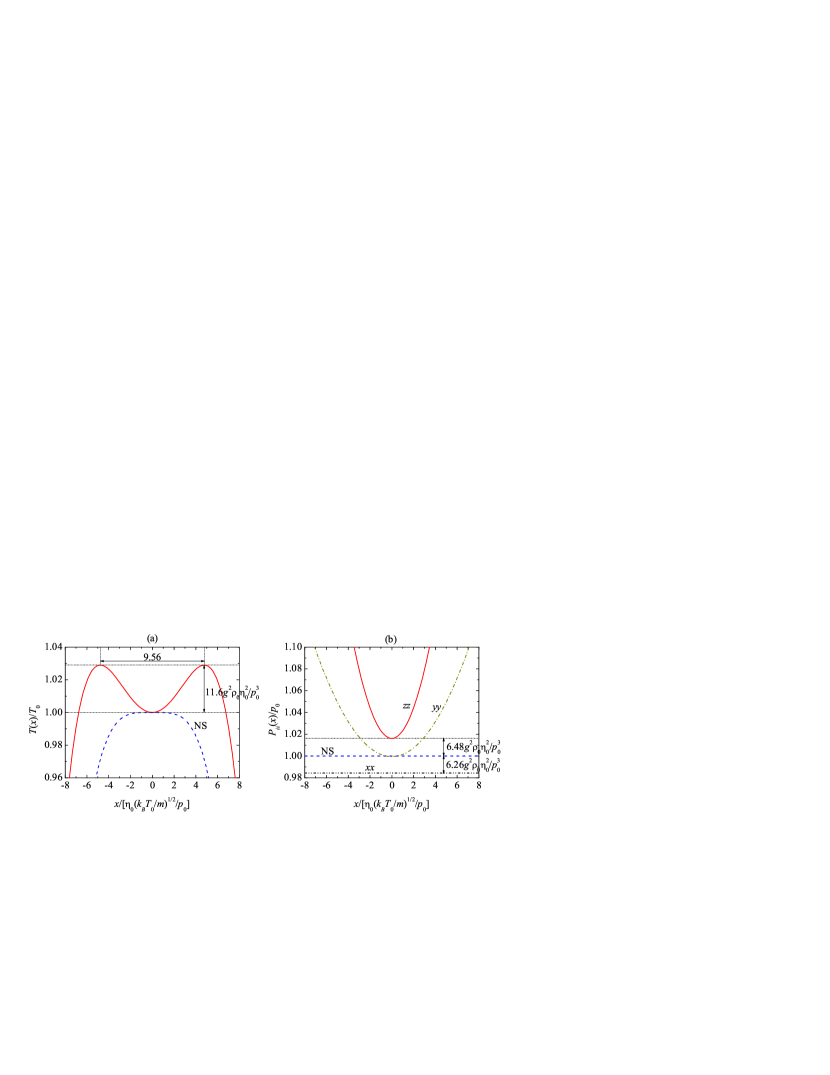
Figure 5: Force-driven Poiseuille flow. Plot of (a) $T(x)/T_{0}$ and (b) $P_{ii}(x)/p_{0}$ for $g=0.05p_{0}^{3/2}/\rho_{0}^{1/2}\eta_{0}$, according to the NS equations and the Boltzmann equation for Maxwell molecules.

All the coefficients $C_{p}$, $C_{T}$, $C_{xx}$, $C_{zz}$, and $C_{q}$ vanish in the NS description ST06 . At a qualitative level, the main correction to the NS results appears for the temperature profile. While, according to the NS equations, the temperature has a maximum at the mid plane $x=0$, the Boltzmann equation shows that, because of the extra quadratic term headed by $C_{T}$, the temperature actually presents a local minimum $T_{0}$ at $x=0$ surrounded by two symmetric maxima $T_{\text{max}}$ at $x=\pm x_{\text{max}}$, where $x_{\text{max}}\equiv\sqrt{6C_{T}\eta_{0}\kappa_{0}T_{0}}/p_{0}$. The relative height of the maxima is $(T_{\text{max}}-T_{0})/T_{0}=2C_{T}(mgx_{\text{max}}/2k_{B}T_{0})^{2}$. Therefore, the temperature does not present a flat maximum at the middle of the channel but instead exhibits a bimodal shape with a local minimum surrounded by two symmetric maxima at a distance of a few mean free paths. This is illustrated by Fig. 5(a) for $g=0.05p_{0}^{3/2}/\rho_{0}^{1/2}\eta_{0}$. The Fourier law is dramatically violated since in the slab enclosed by the two maxima the transverse component of the heat flux is parallel (rather than anti-parallel) to the thermal gradient. Other non-Newtonian effects are the fact that the hydrostatic pressure is not uniform across the system ($C_{p}\neq 0$) and the existence of normal stress differences ($C_{xx}\neq 0$, $C_{zz}\neq 0$), as illustrated by Fig. 5(b) for $g=0.05p_{0}^{3/2}/\rho_{0}^{1/2}\eta_{0}$. Moreover, there exists a heat flux component orthogonal to the thermal gradient ($C_{q}\neq 0$).

The coefficients $C_{p}=\frac{6}{5}=1.2$ and $C_{q}=\frac{2}{5}=0.4$ are already captured by the Burnett description TSS98 ; UG99b . On the other hand, the determination of $C_{T}$, $C_{xx}$, and $C_{zz}$ requires the consideration of, at least, super-Burnett contributions (e.g., $\partial^{3}T/\partial x^{3}$), as first pointed out in Ref. TSS98 . However, a complete determination of those three coefficients requires to retain super-super-Burnett terms (e.g., $\partial^{4}T/\partial x^{4}$). In general, in order to get the fluxes through order $g^{2j}$, one needs to consider the CE expansion though order $2(j+1)$ in the gradients TSS98 ; but this would also provide many extra terms of order higher than $g^{2j}$, that should be discarded. The 13-moment approximation RC98b is able to predict, apart from the correct Burnett-order coefficients $C_{p}$ and $C_{q}$, a non-zero value $C_{T}=\frac{14}{25}=0.56$. The R13-moment approximation significantly improves the value of $C_{T}$ ($C_{T}=\frac{1859}{2000}=0.9295$) and accounts for non-zero values of $C_{xx}$ and $C_{zz}$ ($C_{xx}=\frac{84}{25}=3.36$, $C_{zz}=\frac{256}{75}\simeq 3.413$). Although both values are almost half the correct ones, they satisfactorily show that $C_{zz}$ is only slighter larger than $C_{xx}$, implying that $C_{yy}=-(C_{zz}-C_{xx})$ is rather small. The more complicated 19-moment approximation HM99 gives $C_{T}=\frac{26}{25}=1.04$ for Maxwell molecules but the predictions for $C_{xx}$ and $C_{zz}$ were not explicitly given in Ref. HM99 .

The solution to the BGK equation for the plane Poiseuille flow has been explicitly obtained through order $g^{5}$ TS94 . The results strongly suggest that the series expansion is only asymptotic, so that from a practical point of view one can focus on the first few terms. The results agree with the profiles (120)–(125), except that the numerical values of the coefficients $C_{T}=\frac{19}{25}=0.76$ and, especially, $C_{xx}=\frac{306}{25}=12.24$ and $C_{zz}=\frac{328}{25}=13.12$ differ from those derived from the Boltzmann equation for Maxwell molecules, as shown in Table 5. Interestingly enough, the BGK value of $C_{T}$ agrees quite well with DSMC simulations of the Boltzmann equation for hard spheres MBG97 . It is worth mentioning that an exact, non-perturbative solution of the BGK kinetic model exists for the particular value $g=2.5240p_{0}^{3/2}/\rho_{0}^{1/2}\eta_{0}$ AS92 .

6 Uniform shear flow

The uniform shear flow is a time-dependent state generated by the application of Lees–Edwards boundary conditions LE72 , which are a generalization of the conventional periodic boundary conditions employed in molecular dynamics of systems in equilibrium. Like the Couette flow, the uniform shear flow can be sketched by Fig. 1(b), except that now density and temperature are uniform and the velocity profile is strictly linear GS03 ; T56 ; TM80 . The Boltzmann equation in this state becomes

$$\frac{\partial}{\partial t}f(z,\mathbf{v})+v_{z}\frac{\partial}{\partial z}f(z,\mathbf{v})=J[\mathbf{v}|f,f].$$ (126)

Since there is no thermal gradient, the only hydrodynamic length is $\ell_{u}=\sqrt{2k_{B}T/m}(\partial u_{x}/\partial z)^{-1}$, so that the relevant Knudsen number is the reduced shear rate defined by Eq. (77), which is again constant. On the other hand, in the absence of heat transport, the viscous heating term $P_{xz}\partial u_{x}/\partial z$ cannot be balanced by the divergence of the heat flux and so the temperature monotonically increases with time. In other words, the energy balance equation (79) is replaced by

$$\frac{3nk_{B}}{2}\frac{\partial T}{\partial t}+P_{xz}\frac{\partial u_{x}}{\partial z}=0.$$ (127)

We can still define the dimensionless distribution function (88) and the dimensionless moments (93), but now $\epsilon=0$ (no thermal gradient), so these quantities are nonlinear functions of the reduced shear rate $a$ only. The moment hierarchy is formally similar to Eq. (94), except that the first term on the left-hand side is replaced by a term coming from the time dependence of temperature, in the same way as the first term on the left-hand side of Eq. (79) is replaced by that of Eq. (127). More explicitly, the moment equations are

$$\left(k+\frac{\ell}{2}\right)\xi\overline{M}_{k\ell h}{+a\left(2k\overline{M}_{k-1,\ell+2,h+1}+h\overline{M}_{k,\ell,h-1}\right)}=\frac{1}{\lambdabar_{02}}\overline{J}_{k\ell{h}}({a}),$$ (128)

where $\xi\equiv\lambda_{02}^{-1}\partial\ln T/\partial t$. In contrast to Eq. (94), the hierarchy (128) only couples moments of the same order $2k+\ell$ and of lower order, so it can be solved order by order. Note that moments of odd order (like the heat flux) vanish because of symmetry.

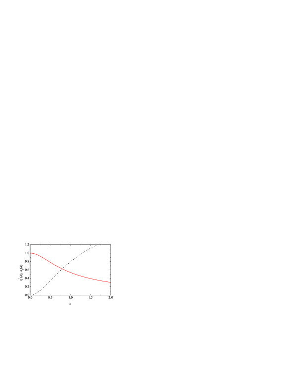
Figure 6: Uniform shear flow. Plot of the nonlinear shear viscosity $\eta^{*}(a)$ (solid line) and the normal stress difference $\Delta_{1}(a)$ (dashed line).

Specifically, setting $(k,\ell,h)=(1,0,0)$, $(0,2,0)$, $(0,2,1)$, and $(0,2,0)$ in Eq. (128), one gets

$$\overline{M}_{020}(a)=\frac{1}{2}\frac{1}{1+\xi(a)},\quad\overline{M}_{021}(a)=-\frac{1}{2}\frac{a}{[1+\xi(a)]^{2}},\quad\overline{M}_{022}(a)=\frac{1}{2}\frac{1+3\xi(a)}{1+\xi(a)},$$ (129)

where $\xi(a)$ is the real root of the cubic equation $3\xi(1+\xi)^{2}=2a^{2}$, namely

$$\xi(a)=\frac{4}{3}\sinh^{2}\left[\frac{1}{6}\cosh^{-1}(1+9a^{2})\right].$$ (130)

Upon deriving Eqs. (129) and (130) use has been made of the properties $\overline{M}_{100}=\frac{3}{2}$, $\overline{J}_{100}=0$, $\overline{J}_{020}=-\lambdabar_{02}\left(\overline{M}_{020}-\frac{1}{2}\right)$, $\overline{J}_{021}=-\lambdabar_{02}\overline{M}_{021}$, and $\overline{J}_{022}=-\lambdabar_{02}\left(\overline{M}_{022}-\frac{1}{2}\right)$.

Figure 7: Uniform shear flow. Plot of the exponent $\tau(a)$ defined by Eq. (132) for the IPL model (solid line) and the VHS model (dashed line). The dotted horizontal line $\tau=2$ intercepts the curves at $a_{c}\simeq 6.846$ and $a_{c}\simeq 7.746$, respectively.

The nonlinear shear viscosity $\eta^{*}(a)$, defined by Eq. (82), and the normal stress differences $\Delta_{1,2}(a)$, defined by Eq. (83), are now explicitly given by

$$\eta^{*}(a)=\frac{1}{[1+\xi(a)]^{2}},\quad\Delta_{1}(a)=\frac{3\xi(a)}{1+\xi(a)},\quad\Delta_{2}(a)=0.$$ (131)

The dependence of $\eta^{*}(a)$ and $\Delta_{1}(a)$ on the reduced shear rate $a$ is shown in Fig. 6. For small shear rates, one has $\xi(a)=\frac{2}{3}a^{2}+\mathcal{O}(a^{4})$, so that $\eta^{*}(a)=1-\frac{4}{3}a^{2}+\mathcal{O}(a^{4})$, $\Delta_{1}(a)=2a^{2}+\mathcal{O}(a^{4})$. The latter two quantities differ from the ones in the Couette flow, Eqs. (106) and (109).

Once the second-order moments are fully determined, one can proceed to the fourth-order moments. Although not related to transport properties, they provide useful information about the population of particles with velocities much larger than the thermal velocity. From Eq. (128) one gets a closed set of nine linear equations that can be algebraically solved GS03 ; SG95 ; SGBD93 . Interestingly, these moments are well-defined only for shear rates smaller than a certain critical value $a_{c}$ ($a_{c}\simeq 6.846$ and $7.746$ for the IPL and VHS models, respectively). Beyond that critical value, the scaled fourth-order moments [e.g., $\langle c^{4}\rangle=\langle V^{4}\rangle/(2k_{B}T/m)^{2}$] monotonically increase in time without upper bound and diverge in the long-time limit. This clearly indicates that the reduced velocity distribution function exhibits an algebraic high-velocity tail GS03 ; MSG96b ; MSG96

$$\phi(\mathbf{c};a)\sim c^{-5-\tau(a)},$$ (132)

so that those moments of order equal to or larger than $2+\tau(a)$ diverge. In particular, the critical shear rate $a_{c}$ is the solution to $\tau(a)=2$. The dependence of the exponent $\tau(a)$ on the shear rate is shown in Fig. 7. The scenario described by Eq. (132) has been confirmed by DSMC results for Maxwell molecules MSG97 . On the other hand, hard spheres do not present an algebraic high-velocity tail MSG96b and thus all the moments are finite.

7 Conclusions

In this paper I have presented an overview of a few cases in which the moment equations stemming from the Boltzmann equation for Maxwell molecules can be used to extract exact information about strongly nonequilibrium properties in the bulk region of the system. This refers to situations where the Knudsen number defined as the ratio between the mean free path and the characteristic distance associated with the hydrodynamic gradients is finite, whilst the ratio between the mean free path and the size of the system is vanishingly small. In other words, the system size comprises many mean free paths but the hydrodynamic quantities can vary appreciably over a distance on the order of the mean free path.

In the conventional Fourier flow problem, the relevant Knudsen number (in the above sense) is given by Eq. (37). Regardless of the value of $\epsilon$, it turns out that the infinite moment hierarchy admits a solution where the pressure is uniform, the temperature is linear in the scaled variable $s$ defined by Eq. (64) [cf. Eq. (66)], and the dimensionless moments of order $\alpha$ are polynomials in $\epsilon$ of degree $\alpha-2$ [cf. Eqs. (53) and (57)]. The latter implies that the dimensional moments of order $\alpha$ are polynomials in $s$ of degree $[\alpha/2]-1$ [cf. Eq. (62)]. In this solution the heat flux is exactly given by Fourier’s law, Eq. (59), even at far from equilibrium states. On the other hand, the situation changes when a gravity field normal to the plates is added. Apart from the Knudsen number $\epsilon$, a relevant parameter is the microscopic Rayleigh number defined by Eq. (67). Assuming $|\gamma|\ll 1$, a perturbation expansion can be carried out about the conventional Fourier flow state, the results exhibiting non-Newtonian effects [cf. Eq. (74)] and a breakdown of Fourier’s law [cf. (75)].

When the parallel plates enclosing the gas are in relative motion, one is dealing with the so-called planar Couette flow. The plates can be kept at the same temperature or at different ones. In the former case the state reduces to that of equilibrium when the plates are at rest, while it reduces to the planar Fourier flow in the latter case. In either situation, the shearing produces a non-uniform heat flux to compensate (in the steady state) for the viscous heating, so that a temperature profile is present. This implies that two independent Knudsen numbers can be identified: the one associated with the flow velocity field [cf. Eq. (77)] and again the one related to the temperature field [cf. Eq. (37)]. Now the exact solution to the moment equations is characterized by a constant pressure, a constant reduced shear rate $a$, a quadratic dependence of the temperature profile on the scaled spatial variable $s$ [cf. Eq. (102)], and again a polynomial dependence of the dimensionless moments on the reduced thermal gradient $\epsilon$ [cf. Eq. (95)]. The dimensional moments of order $\alpha$ are polynomials of degree $\alpha-2$ in $s$ [cf. Eq. (101)]. As a consequence, Newton’s law is modified by a nonlinear shear viscosity [cf. Eq. (82)] and two viscometric functions [cf. Eq. (83)], and a generalized Fourier’s law holds whereby the heat flux is proportional to the thermal gradient but with a nonlinear thermal conductivity [cf. Eq. (85)] and a new coefficient related to the streamwise component [cf. Eq. (99)]. The main difficulty lies in the fact that the coefficients of those polynomials are no longer pure numbers but nonlinear function of the reduced shear rate $a$. Therefore, although the structural form of the solution applies for arbitrary $a$, in order to get explicit results one needs to perform a partial CE expansion in powers of $a$ and get the coefficients recursively. In particular, the super-Burnett coefficients $\eta_{2}^{*}$ and $\kappa_{2}^{*}$ are obtained [cf. Eqs. (106) and (107)].

One of the nonequilibrium states more extensively studied in the last few years is the force-driven Poiseuille flow. A series expansion about the equilibrium state in powers of the external force allows one to get the hydrodynamic profiles and the moments order by order. Calculations to second order suffice to unveil dramatic deviations from the NS predictions. More explicitly, the temperature profile presents a bimodal shape with a dimple at the center of the channel [cf. Fig. 5(a)]. Besides, strong normal-stress differences are present [cf. Fig. 5(b)].

In the specific states summarized above the moment equations have a hierarchical structure since the divergence of the flux term, represented by $\nabla\cdot\bm{\Phi}_{\psi}$ in Eq. (16), involves moments of an order higher than that of $\Psi$. This is what happens in Eqs. (50), (52), (69), (94), and (115). As a consequence, a recursive procedure is needed to obtain explicit results step by step without imposing a truncation closure. On the other hand, the methodology is different (and simpler!) in time-dependent states that become spatially uniform in the co-moving or Lagrangian frame of reference. In that case the divergence of the flux term $\bm{\Phi}_{\psi}$ involves moments of the same order as $\psi$ and so the hierarchical character of the moment equations is truncated in a natural way. This class of states include the uniform shear flow ASB02 ; GS03 ; IT56 ; MS96 ; MSG96 ; SG95 ; SGBD93 ; T56 ; TM80 considered in Sec. 6, and the uniform longitudinal flow (or homoenergetic extension) G95 ; GK96 ; KDN97 ; S00a ; S03 ; TM80 . In both cases the moments of second order (pressure tensor) obey a closed set of autonomous equations that can be algebraically solved to get the rheological properties as explicit nonlinear functions of the reduced velocity gradient, the solution exhibiting interesting non-Newtonian effects. Once the moments of second order are determined, one can proceed to the closed set of equations for the moments of fourth order. Here the interesting result is that those moments diverge beyond a certain critical value of the reduced velocity gradient ASB02 ; GS03 ; S00a ; SGBD93 , what indicates the existence of an algebraic high-velocity tail of the velocity distribution function ASB02 ; GS03 ; MSG96 .

Needless to say, exact results in kinetic theory are important by themselves and also as an assessment of simulation techniques, approximate methods, and kinetic models. In this sense, it is hoped that the states and results reviewed in this paper can become useful to other researchers.

- (1) Abramowitz, M., Stegun, I.A. (eds.): Handbook of Mathematical Functions. Dover, New York (1972)
- (2) Acedo, L., Santos, A., Bobylev, A.V.: On the derivation of a high-velocity tail from the Boltzmann–Fokker–Planck equation for shear flow. J. Stat. Phys. 109, 1027–1050 (2002)
- (3) Alaoui, M., Santos, A.: Poiseuille flow driven by an external force. Phys. Fluids A 4, 1273–1282 (1992)
- (4) Alterman, Z., Frankowski, K., Pekeris, C.L.: Eigenvalues and eigenfunctions of the linearized Boltzmann collision operator for a Maxwell gas and for a gas of rigid spheres. Astrophys. J. Suppl. Ser. 7, 291–331 (1962)
- (5) Ames Research Staff: Equations, Tables and Charts for Compressible Flow. Tech. Rep. 1135, U.S. Ames Aeronautical Laboratory, Moffett Field, CA (1953)
- (6) Anderson, H.L. (ed.): A Physicist’s Desk Reference. American Institute of Physics, New York (1989)
- (7) Andries, P., Le Tallec, P., Perlat, J.P., Perthame, B.: The Gaussian-BGK model of Boltzmann equation with small Prandtl number. Eur. J. Mech. B/Fluids 19, 813–830 (2000)
- (8) Aoki, K., Takata, S., Nakanishi, T.: A Poiseuille-type flow of a rarefied gas between two parallel plates driven by a uniform external force. Phys. Rev. E 65, 026 315 (2002)
- (9) Asmolov, E., Makashev, N.K., Nosik, V.I.: Heat transfer between parallel plates in a gas of Maxwellian molecules. Sov. Phys. Dokl. 24, 892–894 (1979)
- (10) Ben-Naim, E., Krapivsky, P.L.: The inelastic Maxwell model. In: T. Pöschel, S. Luding (eds.) Granular Gases. Springer, Berlin (2003)
- (11) Bhatnagar, P.L., Gross, E.P., Krook, M.: A model for collision processes in gases. I. Small amplitude processes in charged and neutral one-component systems. Phys. Rev. 94, 511–525 (1954)
- (12) Bird, G.: Molecular Gas Dynamics and the Direct Simulation of Gas Flows. Clarendon, Oxford (1994)
- (13) Bobylev, A.V.: The Chapman–Enskog and Grad methods for solving the Boltzmann equation. Sov. Phys. Dokl. 27, 29–31 (1981)
- (14) Brey, J.J., Santos, A., Dufty, J.W.: Heat and momentum transport far from equilibrium. Phys. Rev. A 36, 2842–2849 (1987)
- (15) Brush, S.G.: Kinetic Theory, Vols. I–III. Pergamon Press, London (1965)
- (16) Brush, S.G.: The kind of motion we call heat, Vols. I and II. North–Holland, Amsterdam (1976)
- (17) Brush, S.G.: The Kinetic Theory of Gases. An Anthology of Classic Papers with Historical Commentary. Imperial College Press, London (2003)
- (18) Cercignani, C.: The Boltzmann Equation and Its Applications. Springer–Verlag, New York (1988)
- (19) Cercignani, C.: Mathematical Methods in Kinetic Theory. Plenum Press, New York (1990)
- (20) Cercignani, C., Stefanov, S.: Bénard’s instability in kinetic theory. Transp. Theory Stat. Phys. 21, 371–381 (1992)
- (21) Chapman, S., Cowling, T.G.: The Mathematical Theory of Nonuniform Gases. Cambridge University Press, Cambridge (1970)
- (22) Doi, T., Santos, A., Tij, M.: Numerical study of the influence of gravity on the heat conductivity on the basis of kinetic theory. Phys. Fluids 11, 3553–3559 (1999)
- (23) Dorfman, J.R., van Beijeren, H.: The Kinetic Theory of Gases. In: B.J. Berne (ed.) Statistical Mechanics, Part B, pp. 65–179. Plenum, New York (1977)
- (24) Dufty, J.W.: Kinetic theory of fluids far from equilibrium — Exact results. In: M. López de Haro, C. Varea (eds.) Lectures on Thermodynamics and Statistical Mechanics, pp. 166–181. World Scientific, Singapore (1990)
- (25) Ernst, M.H.: Nonlinear model-Boltzmann equations and exact solutions. Phys. Rep. 78, 1–171 (1981)
- (26) Esposito, R., Lebowitz, J.L., Marra, R.: A hydrodynamic limit of the stationary Boltzmann equation in a slab. Commun. Math. Phys. 160, 49–80 (1994)
- (27) Galkin, V.S.: Exact solution of the system of equations of the second-order kinetic moments for a two-scale homoenergetic affine monatomic gas flow. Fluid Dynamics 30, 467–476 (1995)
- (28) Gallis, M.A., Torczynski, J.R., Rader, D.J., Tij, M., Santos, A.: Normal solutions of the Boltzmann equation for highly nonequilibrium Fourier flow and Couette flow. Phys. Fluids 18, 017,104 (2006)
- (29) Gallis, M.A., Torczynski, J.R., Rader, D.J., Tij, M., Santos, A.: Analytical and Numerical Normal Solutions of the Boltzmann Equation for Highly Nonequilibrium Fourier and Couette Flows. In: M.S. Ivanov, A.K. Rebrov (eds.) Rarefied Gas Dynamics: 25th International Symposium on Rarefied Gas Dynamics, pp. 251–256. Publishing House of the Siberian Branch of the Russian Academy of Sciences, Novosibirsk (2007)
- (30) García-Colín, L.S., Velasco, R.M., Uribe, F.J.: Beyond the Navier-Stokes equations: Burnett hydrodynamics. Phys. Rep. 465, 149 –189 (2008)
- (31) Garzó, V., López de Haro, M.: Nonlinear transport for a dilute gas in steady Couette flow. Phys. Fluids 9, 776–787 (1997)
- (32) Garzó, V., Santos, A.: Kinetic Theory of Gases in Shear Flows. Nonlinear Transport. Kluwer Academic Publishers, Dordrecht (2003)
- (33) Goldstein, H.: Classical Mechanics. Addison–Wesley, Massachusetts (1959)
- (34) Gorban, A.N., Karlin, I.V.: Short-wave limit of hydrodynamics: A soluble example. Phys. Rev. Lett. 77, 282–285 (1996)
- (35) Grad, H.: On the kinetic theory of rarefied gases. Commun. Pure Appl. Math. 2, 331–407 (1949)
- (36) Grad, H.: Asymptotic theory of the Boltzmann equation. Phys. Fluids 6, 147–181 (1963)
- (37) Gradshteyn, I.S., Ryzhik, I.M.: Table of Integrals, Series, and Products. Academic Press, San Diego (1980)
- (38) Hendriks, E.M., Nieuwenhuizen, T.M.: Solution to the nonlinear Boltzmann equation for Maxwell models for nonisotropic initial conditions. J. Stat. Phys. 29, 591–615 (1982)
- (39) Hess, S., Malek Mansour, M.: Temperature profile of a dilute gas undergoing a plane Poiseuille flow. Physica A 272, 481–496 (1999)
- (40) Holway, L.H.: New statistical models for kinetic theory: Methods of construction. Phys. Fluids 9, 1658–1673 (1966)
- (41) Ikenberry, E., Truesdell, C.: On the pressures and the flux of energy in a gas according to Maxwell’s kinetic theory, I. J. Rat. Mech. Anal. 5, 1–54 (1956)
- (42) Kadanoff, L.P., McNamara, G.R., Zanetti, G.: A Poiseuille viscometer for lattice gas automata. Complex Systems 1, 791–803 (1987)
- (43) Kadanoff, L.P., McNamara, G.R., Zanetti, G.: From automata to fluid flow: Comparisons of simulation and theory. Phys.Rev. A 40, 4527–4541 (1989)
- (44) Karlin, I.V., Dukek, G., Nonnenmacher, T.F.: Invariance principle for extension of hydrodynamics: Nonlinear viscosity. Phys. Rev. E 55, 1573–1576 (1997)
- (45) Kim, C.S., Dufty, J.W., Santos, A., Brey, J.J.: Analysis of nonlinear transport in Couette flow. Phys. Rev. A 40, 7165–7174 (1989)
- (46) Kim, C.S., Dufty, J.W., Santos, A., Brey, J.J.: Hilbert-class or “normal” solutions for stationary heat flow. Phys. Rev. A 39, 328–338 (1989)
- (47) Koura, K., Matsumoto, H.: Variable soft sphere molecular model for inverse-power-law or Lennard-Jones potential. Phys. Fluids A 3, 2459–2465 (1991)
- (48) Koura, K., Matsumoto, H.: Variable soft sphere molecular model for air species. Phys. Fluids A 4, 1083–1085 (1992)
- (49) Lees, A.W., Edwards, S.F.: The computer study of transport processes under extreme conditions. J. Phys. C 5, 1921–1929 (1972)
- (50) Makashev, N.K., Nosik, V.I.: Steady Couette flow (with heat transfer) of a gas of Maxwellian molecules. Sov. Phys. Dokl. 25, 589–591 (1981)
- (51) Malek Mansour, M., Baras, F., Garcia, A.L.: On the validity of hydrodynamics in plane Poiseuille flows. Physica A 240, 255–267 (1997)
- (52) McLennan, J.A.: Introduction to Non-Equilibrium Statistical Mechanics. Prentice Hall, Englewood Cliffs, N.J. (1989)
- (53) Montanero, J.M., Alaoui, M., Santos, A., Garzó, V.: Monte Carlo simulation of the Boltzmann equation for steady Fourier flow. Phys. Rev. A 49, 367–375 (1994)
- (54) Montanero, J.M., Garzó, V.: Nonlinear Couette flow in a dilute gas: Comparison between theory and molecular-dynamics simulation. Phys. Rev. E 58, 1836–1842 (1998)
- (55) Montanero, J.M., Santos, A.: Nonequilibrium entropy of a sheared gas. Physica A 225, 7–18 (1996)
- (56) Montanero, J.M., Santos, A., Garzó, V.: Monte Carlo simulation of the Boltzmann equation for uniform shear flow. Phys. Fluids 8, 1981–1983 (1996)
- (57) Montanero, J.M., Santos, A., Garzó, V.: Singular behavior of the velocity moments of a dilute gas under uniform shear flow. Phys. Rev. E 53, 1269–1272 (1996)
- (58) Montanero, J.M., Santos, A., Garzó, V.: Distribution function for large velocities of a two-dimensional gas under shear flow. J. Stat. Phys. 88, 1165–1181 (1997)
- (59) Montanero, J.M., Santos, A., Garzó, V.: Monte Carlo simulation of nonlinear Couette flow in a dilute gas. Phys. Fluids 12, 3060–3073 (2000)
- (60) Nosik, V.I.: Heat transfer between parallel plates in a mixture of gases of Maxwellian molecules. Sov. Phys. Dokl. 25, 495–497 (1981)
- (61) Nosik, V.I.: Degeneration of the Chapman–Enskog expansion in one-dimensional motions of Maxwellian molecule gases. In: O.M. Belotserkovskii, M.N. Kogan, S.S. Kutateladze, A.K. Rebrov (eds.) Rarefied Gas Dynamics 13, pp. 237–244. Plenum Press, New York (1983)
- (62) Résibois, P., de Leener, M.: Classical Kinetic Theory of Fluids. Wiley, New York (1977)
- (63) Risso, D., Cordero, P.: Dilute gas Couette flow: Theory and molecular dynamics simulation. Phys. Rev. E 56, 489–498 (1997)
- (64) Risso, D., Cordero, P.: Erratum: Dilute gas Couette flow: Theory and molecular dynamics simulation. Phys. Rev. E 57, 7365–7366 (1998)
- (65) Risso, D., Cordero, P.: Generalized hydrodynamics for a Poiseuille flow: theory and simulations. Phys. Rev. E 58, 546–553 (1998)
- (66) Sabbane, M., Tij, M.: Calculation algorithm for the collisional moments of the Boltzmann equation for Maxwell molecules. Comp. Phys. Comm. 149, 19–29 (2002)
- (67) Sabbane, M., Tij, M., Santos, A.: Maxwellian gas undergoing a stationary Poiseuille flow in a pipe. Physica A 327, 264–290 (2003)
- (68) Santos, A.: Nonlinear viscosity and velocity distribution function in a simple longitudinal flow. Phys. Rev. E 62, 6597–6607 (2000)
- (69) Santos, A.: Comments on nonlinear viscosity and Grad s moment method. Phys. Rev. E 67, 053 201 (2003)
- (70) Santos, A., Brey, J.J., Dufty, J.W.: An exact solution to the inhomogeneous nonlinear Boltzmann equation. Tech. rep., University of Florida (1987)
- (71) Santos, A., Brey, J.J., Garzó, V.: Kinetic model for steady heat flow. Phys. Rev. A 34, 5047–5050 (1986)
- (72) Santos, A., Brey, J.J., Kim, C.S., Dufty, J.W.: Velocity distribution for a gas with steady heat flow. Phys. Rev. A 39, 320–327 (1989)
- (73) Santos, A., Garzó, V.: Exact moment solution of the Boltzmann equation for uniform shear flow. Physica A 213, 409–425 (1995)
- (74) Santos, A., Garzó, V.: Exact non-linear transport from the Boltzmann equation. In: J. Harvey, G. Lord (eds.) Rarefied Gas Dynamics 19, pp. 13–22. Oxford University Press, Oxford (1995)
- (75) Santos, A., Garzó, V., Brey, J.J., Dufty, J.W.: Singular behavior of shear flow far from equilibrium. Phys. Rev. Lett. 71, 3971–3974 (1993)
- (76) Santos, A., Tij, M.: Gravity-driven Poiseuille Flow in Dilute Gases. Elastic and Inelastic Collisions, chap. 5, pp. 53–67. Nova Science Publishers, New York (2006)
- (77) Söderholm, L.H.: On the Relation between the Hilbert and Chapman-Enskog Expansions. In: T. Abe (ed.) Rarefied Gas Dynamics: Proceedings of the 26th International Symposium on Rarefied Gas Dynamics, pp. 81–86. AIP Conference Proceedings, Volume 1084, Melville, NY (2009)
- (78) Sone, Y., Aoki, K., Sugimoto, H.: The Bénard problem for a rarefied gas: Formation of steady flow patterns and stability of array of rolls. Phys. Fluids 9, 3898–3914 (1997)
- (79) Struchtrup, H.: Macroscopic Transport Equations for Rarefied Gas Flows. Springer, Berlin (2005)
- (80) Struchtrup, H., Torrilhon, M.: Higher-order effects in rarefied channel flows. Phys. Rev. E 78, 046 301 (2008)
- (81) Taheri, P., Torrilhon, M., Struchtrup, H.: Couette and Poiseuille microflows: Analytical solutions for regularized 13-moment equations. Phys. Fluids 21, 017 102 (2009)
- (82) Tahiri, E.E., Tij, M., Santos, A.: Monte Carlo simulation of a hard-sphere gas in the planar Fourier flow with a gravity field. Mol. Phys. 98, 239–248 (2000)
- (83) Tij, M., Garzó, V., Santos, A.: Nonlinear heat transport in a dilute gas in the presence of gravitation. Phys. Rev. E 56, 6729–6734 (1997)
- (84) Tij, M., Garzó, V., Santos, A.: Influence of gravity on nonlinear transport in the planar Couette flow. Phys. Fluids 11, 893–904 (1999)
- (85) Tij, M., Garzó, V., Santos, A.: On the influence of gravity on the thermal conductivity. In: R. Brun, R. Campargue, R. Gatignol, J.C. Lengrand (eds.) Rarefied Gas Dynamics, pp. 239–246. Cépaduès Éditions, Toulouse (1999)
- (86) Tij, M., Sabbane, M., Santos, A.: Nonlinear Poiseuille flow in a gas. Phys. Fluids 10, 1021–1027 (1998)
- (87) Tij, M., Santos, A.: Perturbation analysis of a stationary nonequilibrium flow generated by an external force. J. Stat. Phys. 76, 1399–1414 (1994)
- (88) Tij, M., Santos, A.: Combined heat and momentum transport in a dilute gas. Phys. Fluids 7, 2858–2866 (1995)
- (89) Tij, M., Santos, A.: Non-Newtonian Poiseuille flow of a gas in a pipe. Physica A 289, 336–358 (2001)
- (90) Tij, M., Santos, A.: Poiseuille flow in a heated granular gas. J. Stat. Phys. 117, 901–928 (2004)
- (91) Todd, B.D., Evans, D.J.: Temperature profile for Poiseuille flow. Phys. Rev. E 55, 2800–2807 (1997)
- (92) Travis, K.P., Todd, B.D., Evans, D.J.: Poiseuille flow of molecular fluids. Physica A 240, 315–327 (1997)
- (93) Tritton, D.J.: Physical Fluid Dynamics. Oxford University Press, Oxford (1988)
- (94) Truesdell, C.: On the pressures and the flux of energy in a gas according to Maxwell’s kinetic theory, II. J. Rat. Mech. Anal. 5, 55–128 (1956)
- (95) Truesdell, C., Muncaster, R.G.: Fundamentals of Maxwell’s Kinetic Theory of a Simple Monatomic Gas. Academic Press, New York (1980)
- (96) Uribe, F.J., Garcia, A.L.: Burnett description for plane Poiseuille flow. Phys. Rev. E 60, 4063–4078 (1999)
- (97) Welander, P.: On the temperature jump in a rarefied gas. Arkiv Fysik 7, 507–553 (1954)
- (98) Xu, K.: Super-Burnett solutions for Poiseuille flow. Phys. Fluids 15, 2077–2080 (2003)
- (99) Zheng, Y., Garcia, A.L., Alder, B.J.: Comparison of kinetic theory and hydrodynamics for Poiseuille flow. J. Stat. Phys. 109, 495–505 (2002)