Accurate Noise Projection for Reduced
Stochastic Epidemic Models

Abstract

We consider a stochastic Susceptible-Exposed-Infected-Recovered (SEIR) epidemiological model. Through the use of a normal form coordinate transform, we are able to analytically derive the stochastic center manifold along with the associated, reduced set of stochastic evolution equations. The transformation correctly projects both the dynamics and the noise onto the center manifold. Therefore, the solution of this reduced stochastic dynamical system yields excellent agreement, both in amplitude and phase, with the solution of the original stochastic system for a temporal scale that is orders of magnitude longer than the typical relaxation time. This new method allows for improved time series prediction of the number of infectious cases when modeling the spread of disease in a population. Numerical solutions of the fluctuations of the SEIR model are considered in the infinite population limit using a Langevin equation approach, as well as in a finite population simulated as a Markov process.

The reduction of high-dimensional, stochastic systems is an important and fundamental problem in nonlinear dynamical systems. In this article, we present a general theory of stochastic model reduction which is based on a normal form coordinate transform. This nonlinear, stochastic projection allows for the deterministic and stochastic dynamics to interact correctly on the lower-dimensional manifold so that the dynamics predicted by the reduced, stochastic system agree well with the dynamics predicted by the original, high-dimensional, stochastic system. Although the method may be applied to any physical or biological system with well-separated time scales, here we apply the method to an epidemiological model. We show that when compared to the original, stochastic epidemic model, the reduced model properly captures the initial and recurrent disease outbreaks, both in amplitude and phase. This long-term accuracy of the reduced model allows for the application of effective disease control where phase differences between outbreak times and vaccine controls are important. Additionally, in practice, one can only measure the number of infectious individuals in a population. Our method allows one to predict the number of unobserved exposed individuals based on the observed number of infectious individuals.

I Introduction

The interaction between deterministic and stochastic effects in population dynamics has played, and continues to play, an important role in the modeling of infectious diseases. The mechanistic modeling side of population dynamics is well-known and established Anderson91 ; bailey75 . These models typically are assumed to be useful for infinitely large, homogeneous populations, and arise from the mean field analysis of probabilistic models. On the other hand, when one considers finite populations, random interactions give rise to internal noise effects, which may introduce new dynamics. Stochastic effects are quite prominent in finite populations, which can range from ecological dynamics Marion2000 to childhood epidemics in cities Nguyen2008 ; Rohani2002 . For homogeneous populations with seasonal forcing, noise also comes into play in the prediction of large outbreaks Rand1991 ; BillingsBS02 ; stolhu07 . Specifically, external random perturbations change the probabilistic prediction of epidemic outbreaks as well as its control Schwartz2004 .

When geometric structure is applied to the population, the interactions are modeled as a network Pastor-SatorrasV01 ; moreno2002 . Many types of static networks which support epidemics have been considered. Some examples include small world networks Vazquez06 , hierarchical networks WattsMMD05 , and transportation networks of patch models ColizzaBBV06 . In addition, the fluctuation of epidemics on adaptive networks, where the wiring between nodes changes in response to the node information, has been examined shasch08 . In adaptive network models, even the mean field can be high-dimensional, since nodes and links evolve in time and must be approximated as an additional set of ordinary differential equations.

Another aspect of epidemic models which is often of interest involves the inclusion of a time delay. The delay term makes the analysis significantly more complicated. However, it is possible to approximate the delay by creating a cascade consisting of a large number of compartments mrv05 . For example, one could simulate the delay associated with a disease exposure time with several hundred “exposed” compartments.

These model examples are just a few of the types of very high-dimensional models that are currently of interest. As a result of the high-dimensionality, there is much computation involved, and the analysis is quite difficult. In particular, real-time computation is not currently possible. However, there are usually many time scales that are well-separated (due typically to a large range in order of magnitude of the parameters) when considering such high-dimensional problems. In the presence of well-separated time scales, a model reduction method is needed to examine the dynamics on a lower-dimensional space. It is known that deterministic model reduction methods may not work well in the stochastic realm, which includes epidemic models forsch09 . The purpose of this article is to examine a method of nonlinear, stochastic projection so that the deterministic and stochastic dynamics interact correctly on the lower-dimensional manifold and predict correctly the dynamics when compared to the full system. Because the noise affects the timing of outbreaks, it is essential to produce a low-dimensional system which captures the correct timing of the outbreaks as well as the amplitude and phase of any recurrent behavior.

We will demonstrate that our stochastic model reduction method properly captures the initial disease outbreak and continues to accurately predict the outbreaks for time scales which are orders of magnitude longer than the typical relaxation time. Furthermore, in practice, real disease data includes only the number of infectious individuals. Our method allows us to predict the number of unobserved exposed individuals based on the observed number of infectious individuals.

For stochastic model reduction, there exist several potential methods for general problems. For a system with certain spectral requirements, the existence of a stochastic center manifold was proven in Ref. box89, . Non-rigorous stochastic normal form analysis (which leads to the stochastic center manifold) was performed in Refs. coelti85, ; knowie83, ; nam90, ; namlin91, . Rigorous theoretical analysis of normal form coordinate transformations for stochastic center manifold reduction was developed in Refs. arn98, ; arnimk98, . Later, another method of stochastic normal form reduction was developed rob08 , in which any anticipatory convolutions (integrals into the future of the noise processes) that appeared in the slow modes were removed. Since this latter analysis makes the construction of the stochastic normal form coordinate transform more transparent, we use this method to derive the reduced stochastic center manifold equation.

Figure 1 shows a schematic demonstrating our approach to the problem. We consider a high-dimensional system along with its corresponding reduced low-dimensional system. In this article, two types of low-dimensional system are discussed: a reduced system based on deterministic center manifold analysis and a reduced system based on a stochastic normal form coordinate transform. Regardless of the type of low-dimensional system being considered, a common noise is injected into both the high-dimensional and low-dimensional models, and an analysis of the solutions found using the high and low-dimensional systems is performed.

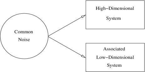
Figure 1: Schematic demonstrating the injection of a common noise into both the high-dimensional system and its associated low-dimensional system.

In this article, as a first study of a high-dimensional system, we consider the Susceptible-Exposed-Infected-Recovered (SEIR) epidemiological model with stochastic forcing. As previously mentioned, we could easily consider a SEIR-type model where the exposed class was modeled using hundreds of compartments. Since the analysis is similar, we consider the simpler standard SEIR model to demonstrate the power of our method. Section II provides a complete description of this model. Section III describes how to transform the deterministic SEIR system to a new system that satisfies the spectral requirements needed to apply the center manifold theory. After the theory is used to find the evolution equations that describe the dynamics on the center manifold, we show in Sec. IV how the reduced model that is found using the deterministic result incorrectly projects the noise onto the center manifold. Section V demonstrates the use of a stochastic normal form coordinate transform to correctly project the noise onto the stochastic center manifold. A discussion section and the conclusions are contained respectively in Sec. VI and Sec. VII.

II The SEIR model for epidemics

We begin by describing the stochastic version of the SEIR model found in Ref. ss83, . We assume that a given population may be divided into the following four classes which evolve in time:

1. Susceptible class, $s(t)$, consists of those individuals who may contract the disease.

2. Exposed class, $e(t)$, consists of those individuals who have been infected by the disease but are not yet infectious.

3. Infectious class, $i(t)$, consists of those individuals who are capable of transmitting the disease to susceptible individuals.

4. Recovered class, $r(t)$, consists of those individuals who are immune to the disease.

Furthermore, we assume that the total population size, denoted as $N$, is constant and can be normalized to $S(t)+E(t)+I(t)+R(t)=1$, where $S(t)=s(t)/N$, $E(t)=e(t)/N$, $I(t)=i(t)/N$, and $R(t)=r(t)/N$. Therefore, the population class variables $S$, $E$, $I$, and $R$ represent fractions of the total population. The governing equations for the stochastic SEIR model are

$$\dot{S}(t)=\mu-\beta I(t)S(t)-\mu S(t)+\sigma_{1}\phi_{1}(t),$$ (1a)

$$\dot{E}(t)=\beta I(t)S(t)-(\alpha+\mu)E(t)+\sigma_{2}\phi_{2}(t),$$ (1b)

$$\dot{I}(t)=\alpha E(t)-(\gamma+\mu)I(t)+\sigma_{3}\phi_{3}(t),$$ (1c)

$$\dot{R}(t)=\gamma I(t)-\mu R(t)+\sigma_{4}\phi_{4}(t),$$ (1d)

where $\sigma_{i}$ is the standard deviation of the noise intensity $D_{i}=\sigma_{i}^{2}/2$. Each of the noise terms, $\phi_{i}$, describes a stochastic, Gaussian white force that is characterized by the correlation functions

$$\langle\phi_{i}(t)\rangle=0,$$ (2a)

$$\langle\phi_{i}(t)\phi_{j}(t^{\prime})\rangle=\delta(t-t^{\prime})\delta_{ij}.$$ (2b)

Additionally, $\mu$ represents a constant birth and death rate, $\beta$ is the contact rate, $\alpha$ is the rate of infection, so that $1/\alpha$ is the mean latency period, and $\gamma$ is the rate of recovery, so that $1/\gamma$ is the mean infectious period. Although the contact rate $\beta$ could be given by a time-dependent function (e.g. due to seasonal fluctuations), for simplicity, we assume $\beta$ to be constant. Throughout this article, we use the following parameter values: $\mu=0.02({\rm year})^{-1}$, $\beta=1575.0({\rm year})^{-1}$, $\alpha=1/0.0279({\rm year})^{-1}$, and $\gamma=1/0.01({\rm year})^{-1}$. Disease parameters correspond to typical measles values ss83 ; bisc02 . Note that any other biologically meaningful parameters may be used as long as the basic reproductive rate $R_{0}=\alpha\beta/[(\alpha+\mu)(\gamma+\mu)]>1$. The interpretation of $R_{0}$ is the number of secondary cases produced by a single infectious individual in a population of susceptibles in one infectious period.

As a first approximation of stochastic effects, we have considered additive noise. This type of noise may result from migration into and away from the population being considered BvdDW08 . Since it is difficult to estimate fluctuating migration rates bfg02 , it is appropriate to treat migration as an arbitrary external noise source. Also, fluctuations in the birth rate manifest itself as additive noise. Furthermore, as we are not interested in extinction events in this article, it is not necessary to use multiplicative noise. In general, for the problem considered here, it is possible that a rare event in the tail of the noise distribution may cause one or more of the $S$, $E$, and $I$ components of the solution to become negative. In this article, we will always assume that the noise is sufficiently small so that a solution remains positive for a long enough time to gather sufficient statistics. Even though it is difficult to accurately estimate the appropriate noise level from real data, our choices of noise intensity lie within the huge confidence intervals computed in Ref. bfg02, . The case for multiplicative noise will be considered in a separate paper.

Although $S+E+I+R=1$ in the deterministic system, one should note that the dynamics of the stochastic SEIR system will not necessarily have all of the components sum to unity. However, since the noise has zero mean, the total population will remain close to unity on average. Therefore, we assume that the dynamics are sufficiently described by Eqs. (1a)-(1c). It should be noted that even if $E(t)+I(t)=0$ for some $t$, the noise allows for the reemergence of the epidemic.

III Deterministic center manifold analysis

One way to reduce the dimension of a system of equations is through the use of deterministic center manifold theory. In general, a nonlinear vector field can be transformed so that the linear part (Jacobian) of the vector field has block diagonal form where the first matrix block has eigenvalues with positive real part, the second matrix block has eigenvalues with negative real part, and the third matrix block has eigenvalues with zero real part hirsma74 ; wig90 . These blocks are associated respectively with the unstable eigenspace, the stable eigenspace, and the center eigenspace. If we suppose that there are no eigenvalues with positive real part, then orbits will rapidly decay to the center eigenspace.

In order to make use of the center manifold theory, we must transform Eqs. (1a)-(1c) to a new system of equations that has the necessary spectral structure. The theory will allow us to find an invariant center manifold passing through the fixed point to which we can restrict the transformed system. Details regarding the transformation can be found in Sec. III.1, and the computation of the center manifold can be found in Sec. III.2.

III.1 Transformation of the SEIR model

Our analysis begins by considering the governing equations for the stochastic SEIR model given by Eqs. (1a)-(1c). We neglect the $\sigma_{i}\phi_{i}(t)$ terms in Eqs. (1a)-(1c) so that we are considering the deterministic SEIR system. This deterministic system has two fixed points. The first fixed point is

$$(S_{e},E_{e},I_{e})=(1,0,0),$$ (3)

and corresponds to a disease free, or extinct, equilibrium state. The second fixed point corresponds to an endemic state and is given by

$$(S_{0},E_{0},I_{0})=\left({\frac{\left(\gamma+\mu\right)\left(\alpha+\mu\right)}{\beta\alpha}},{\frac{\mu}{\alpha+\mu}}-{\frac{\mu\left(\gamma+\mu\right)}{\alpha\beta}},{\frac{\mu\alpha}{\left(\gamma+\mu\right)\left(\alpha+\mu\right)}}-{\frac{\mu}{\beta}}\right).$$ (4)

To ease the analysis, we define a new set of variables, $\bar{S}$, $\bar{E}$, and $\bar{I}$, as $\bar{S}(t)=S(t)-S_{0}$, $\bar{E}(t)=E(t)-E_{0}$, and $\bar{I}(t)=I(t)-I_{0}$. These new variables are substituted into Eqs. (1a)-(1c).

Then, treating $\mu$ as a small parameter, we rescale time by letting $t=\mu\tau$. We may then introduce the following rescaled parameters: $\alpha=\alpha_{0}/\mu$ and $\gamma=\gamma_{0}/\mu$, where $\alpha_{0}$ and $\gamma_{0}$ are $\mathcal{O}(1)$. The inclusion of the parameter $\mu$ as a new state variable means that the terms in our rescaled system which contain $\mu$ are now nonlinear terms. Furthermore, the system is augmented with the auxiliary equation $\frac{d\mu}{d\tau}=0$. The addition of this auxiliary equation contributes an extra simple zero eigenvalue to the system and adds one new center direction that has trivial dynamics. The shifted and rescaled, augmented system of equations is

$$\frac{d\bar{S}}{d\tau}= -\beta\mu\bar{I}\bar{S}-\frac{(\alpha_{0}+\mu^{2})(\gamma_{0}+\mu^{2})}{\alpha_{0}}\bar{I}-\frac{\alpha_{0}\mu^{3}\beta}{(\alpha_{0}+\mu^{2})(\gamma_{0}+\mu^{2})}\bar{S},$$ (5a)

$$\frac{d\bar{E}}{d\tau}= \beta\mu\bar{I}\bar{S}+\frac{(\alpha_{0}+\mu^{2})(\gamma_{0}+\mu^{2})}{\alpha_{0}}\bar{I}+\frac{\mu^{2}[\alpha_{0}\beta\mu-(\alpha_{0}+\mu^{2})(\gamma_{0}+\mu^{2})]}{(\alpha_{0}+\mu^{2})(\gamma_{0}+\mu^{2})}\bar{S}-(\alpha_{0}+\mu^{2})\bar{E},$$ (5b)

$$\frac{d\bar{I}}{d\tau}= \alpha_{0}\bar{E}-(\gamma_{0}+\mu^{2})\bar{I},$$ (5c)

$$\frac{d\mu}{d\tau}= 0,$$ (5d)

where the endemic fixed point is now located at the origin.

The Jacobian of Eqs. (5a)-(5d) is computed to zeroth-order in $\mu$ and is evaluated at the origin. Ignoring the $\mu$ components, the Jacobian has only two linearly independent eigenvectors. Therefore, the Jacobian is not diagonalizable. However, it is possible to transform Eqs. (5a)-(5c) to a block diagonal form with the eigenvalue structure that is needed to use center manifold theory. We use a transformation matrix, ${\bf P}$, consisting of the two linearly independent eigenvectors of the Jacobian along with a third vector chosen to be linearly independent. There are many choices for this third vector; our choice is predicated on keeping the vector as simple as possible. This transformation matrix is given as

$${\bf P}=\left[\begin{array}[]{cccccccc}1&&&1&&&&0\\ &&&&&&&\\ -\frac{\alpha_{0}+\gamma_{0}}{\gamma_{0}}&&&0&&&&0\\ &&&&&&&\\ \frac{\alpha_{0}+\gamma_{0}}{\gamma_{0}}&&&0&&&&1\\ \end{array}\right].$$ (6)

Using the fact that $(\bar{S},\bar{E},\bar{I})^{T}={\bf P}\cdot(U,V,W)^{T}$, then the transformation matrix leads to the following definition of new variables, $U$, $V$, and $W$:

$$U=\frac{-\gamma_{0}}{\alpha_{0}+\gamma_{0}}\bar{E},$$ (7a)

$$V=\bar{S}+\frac{\gamma_{0}}{\alpha_{0}+\gamma_{0}}\bar{E},$$ (7b)

$$W=\bar{I}+\bar{E}.$$ (7c)

The application of the transformation matrix to Eqs. (5a)-(5c) leads to the transformed evolution equations given by

$$\frac{dU}{d\tau}= -\alpha_{0}U+{\frac{\mu^{2}\left(\gamma_{0}V-\alpha_{0}U\right)}{\alpha_{0}+\gamma_{0}}}-{\frac{\left(\gamma_{0}+\mu^{2}\right)\left(\alpha_{0}+\mu^{2}\right)\left[\left(\alpha_{0}+\gamma_{0}\right)U+\gamma_{0}W\right]}{\alpha_{0}\left(\alpha_{0}+\gamma_{0}\right)}}-$$

$$\frac{\mu\beta}{\alpha_{0}+\gamma_{0}}\left(\gamma_{0}W+\left(\alpha_{0}+\gamma_{0}\right)U+{\frac{\mu^{2}\alpha_{0}\gamma_{0}}{\left(\gamma_{0}+\mu^{2}\right)\left(\alpha_{0}+\mu^{2}\right)}}\right)\left(U+V\right),$$ (8a)

$$\frac{dV}{d\tau}= \alpha_{0}U-{\frac{\mu^{2}\left(\gamma_{0}V-\alpha_{0}U\right)}{\alpha_{0}+\gamma_{0}}}-{\frac{\left(\gamma_{0}+\mu^{2}\right)\left(\alpha_{0}+\mu^{2}\right)\left[\left(\alpha_{0}+\gamma_{0}\right)U+\gamma_{0}W\right]}{\gamma_{0}\left(\alpha_{0}+\gamma_{0}\right)}}-$$

$$\frac{\mu\beta\alpha_{0}}{\gamma_{0}\left(\alpha_{0}+\gamma_{0}\right)}\left(\gamma_{0}W+\left(\alpha_{0}+\gamma_{0}\right)U+{\frac{\mu^{2}\alpha_{0}\gamma_{0}}{\left(\gamma_{0}+\mu^{2}\right)\left(\alpha_{0}+\mu^{2}\right)}}\right)\left(U+V\right),$$ (8b)

$$\frac{dW}{d\tau}= -\alpha_{0}U-\left(\gamma_{0}+\mu^{2}\right)\left(U+W\right)+{\frac{\left(\gamma_{0}+\mu^{2}\right)\left(\alpha_{0}+\mu^{2}\right)\left[\left(\alpha_{0}+\gamma_{0}\right)U+\gamma_{0}W\right]}{\alpha_{0}\gamma_{0}}}-$$

$$\mu^{2}V+\frac{\mu\beta}{\gamma_{0}}\left(\gamma_{0}W+\left(\alpha_{0}+\gamma_{0}\right)U+{\frac{\mu^{2}\alpha_{0}\gamma_{0}}{\left(\gamma_{0}+\mu^{2}\right)\left(\alpha_{0}+\mu^{2}\right)}}\right)\left(U+V\right),$$ (8c)

$$\frac{d\mu}{d\tau}= 0.$$ (8d)

III.2 Center manifold equation

The Jacobian of Eqs. (8a)-(8d) to zeroth-order in $\mu$ and evaluated at the origin is

$$\left[\begin{array}[]{cc|ccccccccc}-(\alpha_{0}+\gamma_{0})&&&&0&&&-\frac{\gamma_{0}^{2}}{(\alpha_{0}+\gamma_{0})}&&&0\\ &&&&&&&&&&\\ \hline\cr&&&&&&&&&&\\ 0&&&&0&&&-\frac{\alpha_{0}\gamma_{0}}{(\alpha_{0}+\gamma_{0})}&&&0\\ &&&&&&&&&&\\ 0&&&&0&&&0&&&0\\ &&&&&&&&&&\\ 0&&&&0&&&0&&&0\end{array}\right],$$ (9)

which shows that Eqs. (8a)-(8d) may be rewritten in the form

$$\frac{d{\bf x}}{d\tau}={\bf A}{\bf x}+{\bf f}({\bf x},{\bf y},\mu),$$ (10)

$$\frac{d{\bf y}}{d\tau}={\bf B}{\bf y}+{\bf g}({\bf x},{\bf y},\mu),$$ (11)

$$\frac{d\mu}{d\tau}=0,$$ (12)

where ${\bf x}=(U)$, ${\bf y}=(V,W)$, ${\bf A}$ is a constant matrix with eigenvalues that have negative real parts, ${\bf B}$ is a constant matrix with eigenvalues that have zero real parts, and ${\bf f}$ and ${\bf g}$ are nonlinear functions in ${\bf x}$, ${\bf y}$ and $\mu$. In particular,

$${\bf A}=\left[\begin{array}[]{c}-(\alpha_{0}+\gamma_{0})\end{array}\right],\,\,\,\,\,\,\,\,\,\,\,\,\,\,\,{\bf B}=\left[\begin{array}[]{cccc}0&&&-\frac{\alpha_{0}\gamma_{0}}{(\alpha_{0}+\gamma_{0})}\\ &&&\\ 0&&&0\end{array}\right].$$ (13)

Therefore, the system will rapidly collapse onto a lower-dimensional manifold given by center manifold theory car81 . Furthermore, we know that the center manifold is given by

$$U=h(V,W,\mu),$$ (14)

where $h$ is an unknown function.

Substitution of Eq. (14) into Eq. (8a) leads to the following center manifold condition:

$$\frac{\partial h(V,W,\mu)}{\partial V}\frac{dV}{d\tau}+\frac{\partial h(V,W,\mu)}{\partial W}\frac{dW}{d\tau}=-\alpha_{0}h(V,W,\mu)+{\frac{\mu^{2}\left[\gamma_{0}V-\alpha_{0}h(V,W,\mu)\right]}{\alpha_{0}+\gamma_{0}}}-$$

$${\frac{\left(\gamma_{0}+\mu^{2}\right)\left(\alpha_{0}+\mu^{2}\right)\left[\left(\alpha_{0}+\gamma_{0}\right)h(V,W,\mu)+\gamma_{0}W\right]}{\alpha_{0}\left(\alpha_{0}+\gamma_{0}\right)}}-$$

$$\frac{\mu\beta}{\alpha_{0}+\gamma_{0}}\left(\gamma_{0}W+\left(\alpha_{0}+\gamma_{0}\right)h(V,W,\mu)+{\frac{\mu^{2}\alpha_{0}\gamma_{0}}{\left(\gamma_{0}+\mu^{2}\right)\left(\alpha_{0}+\mu^{2}\right)}}\right)\left(h(V,W,\mu)+V\right).$$ (15)

In general, it is not possible to solve the center manifold condition for the unknown function, $h(V,W,\mu)$. Therefore, we perform the following Taylor series expansion of $h(V,W,\mu)$ in $V$, $W$, and $\mu$:

$$h(V,W,\mu)= h_{0}+h_{2}V+h_{3}W+h_{\mu}\mu+h_{22}V^{2}+h_{23}VW+h_{33}W^{2}+$$

$$h_{\mu 2}\mu V+h_{\mu 3}\mu W+h_{\mu\mu}\mu^{2}+\ldots,$$ (16)

where $h_{0}$, $h_{2}$, $h_{3}$, $h_{\mu}$, $\ldots$ are unknown coefficients that are found by substituting the Taylor series expansion into the center manifold condition and equating terms of the same order. By carrying out this procedure using a second-order Taylor series expansion of $h$, the center manifold equation is

$$U=-\frac{\gamma_{0}^{2}}{(\alpha_{0}+\gamma_{0})^{2}}W+\mathcal{O}(\epsilon^{3}),$$ (17)

where $\epsilon=|(V,W,\mu)|$ so that $\epsilon$ provides a count of the number of $V$, $W$, and $\mu$ factors in any one term. Substitution of Eq. (17) into Eqs. (8b) and (8c) leads to the following reduced system of evolution equations which describe the dynamics on the center manifold:

$$\frac{dV}{d\tau}= -{\frac{\mu^{2}{\gamma_{0}}^{2}\alpha_{0}W}{\left(\alpha_{0}+\gamma_{0}\right)^{3}}}-{\frac{\mu^{4}\alpha_{0}W}{\left(\alpha_{0}+\gamma_{0}\right)^{2}}}-{\frac{\gamma_{0}\mu^{2}V}{\alpha_{0}+\gamma_{0}}}-$$

$${\frac{\left(\gamma_{0}+\mu^{2}\right)\alpha_{0}W}{\alpha_{0}+\gamma_{0}}}-\frac{\beta{\alpha_{0}}^{2}\mu}{\left(\alpha_{0}+\gamma_{0}\right)^{2}}\left(W+{\frac{\mu^{2}\left(\alpha_{0}+\gamma_{0}\right)}{\left(\gamma_{0}+\mu^{2}\right)\left(\alpha_{0}+\mu^{2}\right)}}\right)\left(V-{\frac{{\gamma_{0}}^{2}W}{\left(\alpha_{0}+\gamma_{0}\right)^{2}}}\right),$$ (18a)

$$\frac{dW}{d\tau}= {\frac{\mu^{2}{\gamma_{0}}^{2}W}{\left(\alpha_{0}+\gamma_{0}\right)^{2}}}+{\frac{\mu^{4}W}{\alpha_{0}+\gamma_{0}}}-\mu^{2}V+$$

$$\frac{\beta\mu\alpha_{0}}{\alpha_{0}+\gamma_{0}}\left(W+{\frac{\mu^{2}\left(\alpha_{0}+\gamma_{0}\right)}{\left(\gamma_{0}+\mu^{2}\right)\left(\alpha_{0}+\mu^{2}\right)}}\right)\left(V-{\frac{{\gamma_{0}}^{2}W}{\left(\alpha_{0}+\gamma_{0}\right)^{2}}}\right).$$ (18b)

IV Incorrect projection of the noise onto the stochastic center manifold

IV.1 Transformation of the stochastic SEIR model

We now return to the stochastic SEIR system given by Eqs. (1a)-(1c). The shift of the fixed point to the origin will not have any effect on the noise terms, so that the stochastic version of the shifted equations is

$$\dot{\bar{S}}(t)=-\beta\bar{I}\bar{S}-\frac{(\alpha+\mu)(\gamma+\mu)}{\alpha}\bar{I}-\frac{\alpha\mu\beta}{(\alpha+\mu)(\gamma+\mu)}\bar{S}+\sigma_{1}\phi_{1}(t),$$ (19a)

$$\dot{\bar{E}}(t)=\beta\bar{I}\bar{S}+\frac{(\alpha+\mu)(\gamma+\mu)}{\alpha}\bar{I}+\frac{\mu[\alpha\beta-(\alpha+\mu)(\gamma+\mu)]}{(\alpha+\mu)(\gamma+\mu)}\bar{S}-(\alpha+\mu)\bar{E}+\sigma_{2}\phi_{2}(t),$$ (19b)

$$\dot{\bar{I}}(t)=\alpha\bar{E}-(\gamma+\mu)\bar{I}+\sigma_{3}\phi_{3}(t).$$ (19c)

As Eqs. (19a)-(19c) are transformed using Eqs. (7a)-(7c), the $\alpha=\alpha_{0}/\mu$ scaling, the $\gamma=\gamma_{0}/\mu$ scaling, and the $t=\mu\tau$ time scaling, the noise also is scaled so that the stochastic, transformed equations are given by

$$\frac{dU}{d\tau}= -\alpha_{0}U+{\frac{\mu^{2}\left(\gamma_{0}V-\alpha_{0}U\right)}{\alpha_{0}+\gamma_{0}}}-{\frac{\left(\gamma_{0}+\mu^{2}\right)\left(\alpha_{0}+\mu^{2}\right)\left[\left(\alpha_{0}+\gamma_{0}\right)U+\gamma_{0}W\right]}{\alpha_{0}\left(\alpha_{0}+\gamma_{0}\right)}}-$$

$$\frac{\mu\beta}{\alpha_{0}+\gamma_{0}}\left(\gamma_{0}W+\left(\alpha_{0}+\gamma_{0}\right)U+{\frac{\mu^{2}\alpha_{0}\gamma_{0}}{\left(\gamma_{0}+\mu^{2}\right)\left(\alpha_{0}+\mu^{2}\right)}}\right)\left(U+V\right)+\sigma_{4}\phi_{4},$$ (20a)

$$\frac{dV}{d\tau}= \alpha_{0}U-{\frac{\mu^{2}\left(\gamma_{0}V-\alpha_{0}U\right)}{\alpha_{0}+\gamma_{0}}}-{\frac{\left(\gamma_{0}+\mu^{2}\right)\left(\alpha_{0}+\mu^{2}\right)\left[\left(\alpha_{0}+\gamma_{0}\right)U+\gamma_{0}W\right]}{\gamma_{0}\left(\alpha_{0}+\gamma_{0}\right)}}-$$

$$\frac{\mu\beta\alpha_{0}}{\gamma_{0}\left(\alpha_{0}+\gamma_{0}\right)}\left(\gamma_{0}W+\left(\alpha_{0}+\gamma_{0}\right)U+{\frac{\mu^{2}\alpha_{0}\gamma_{0}}{\left(\gamma_{0}+\mu^{2}\right)\left(\alpha_{0}+\mu^{2}\right)}}\right)\left(U+V\right)+\sigma_{5}\phi_{5},$$ (20b)

$$\frac{dW}{d\tau}= -\alpha_{0}U-\left(\gamma_{0}+\mu^{2}\right)\left(U+W\right)+{\frac{\left(\gamma_{0}+\mu^{2}\right)\left(\alpha_{0}+\mu^{2}\right)\left[\left(\alpha_{0}+\gamma_{0}\right)U+\gamma_{0}W\right]}{\alpha_{0}\gamma_{0}}}-$$

$$\mu^{2}V+\frac{\mu\beta}{\gamma_{0}}\left(\gamma_{0}W+\left(\alpha_{0}+\gamma_{0}\right)U+{\frac{\mu^{2}\alpha_{0}\gamma_{0}}{\left(\gamma_{0}+\mu^{2}\right)\left(\alpha_{0}+\mu^{2}\right)}}\right)\left(U+V\right)+\sigma_{6}\phi_{6},$$ (20c)

where

$$\sigma_{4}\phi_{4}= -\frac{\mu\gamma_{0}}{\alpha_{0}+\gamma_{0}}\sigma_{2}\phi_{2},$$ (21a)

$$\sigma_{5}\phi_{5}= \mu\sigma_{1}\phi_{1}+\frac{\mu\gamma_{0}}{\alpha_{0}+\gamma_{0}}\sigma_{2}\phi_{2},$$ (21b)

$$\sigma_{6}\phi_{6}= \mu\sigma_{2}\phi_{2}+\mu\sigma_{3}\phi_{3}.$$ (21c)

The stochastic terms $\phi_{4}$, $\phi_{5}$, and $\phi_{6}$ in Eqs. (20a)-(20c) are still additive, Gaussian noise processes. However, Eqs. (21a)-(21c) show how the transformation has acted on the original stochastic terms $\phi_{1}$, $\phi_{2}$, and $\phi_{3}$ to create new noise processes which have a variance different from that of the original noise processes. Also note that we have suppressed the argument of $\phi_{4}$, $\phi_{5}$, and $\phi_{6}$ in Eqs. (20a)-(20c). The time scaling means that these noise terms should be evaluated at $\mu\tau$.

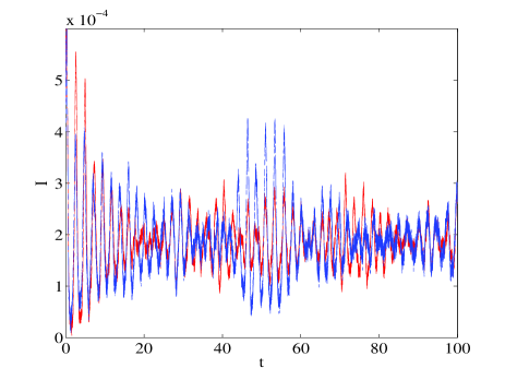
Figure 2: (Color online) Time series of the fraction of the population that is infected with a disease, $I$, computed using the original, stochastic system of equations of the SEIR model [Eqs. (1a)-(1c)] (red, solid line), and computed using the transformed, stochastic system of equations of the SEIR model [Eqs. (20a)-(20c)] (blue, dashed line). The standard deviation of the noise intensity used in the simulation is $\sigma_{i}=0.0005$, $i=1,\ldots,6$.

The system of equations given by Eqs. (20a)-(21c) are an exact transformation of the system of equations given by Eqs. (1a)-(1c). We numerically integrate the original, stochastic system of the SEIR model [Eqs. (1a)-(1c)] along with the transformed, stochastic system [Eqs. (20a)-(20c)] using a stochastic fourth-order Runge-Kutta scheme with a constant time step size. The original system is solved for $S$, $E$, and $I$, while the transformed system is solved for $U$, $V$, and $W$. In the latter case, once the values of $U$, $V$, and $W$ are known, we compute the values of $\bar{S}$, $\bar{E}$, and $\bar{I}$ using the transformation given by Eqs. (7a)-(7c). We shift $\bar{S}$, $\bar{E}$, and $\bar{I}$ respectively by $S_{0}$, $E_{0}$, and $I_{0}$ to find the values of $S$, $E$, and $I$.

Figure 2 compares the time series of the fraction of the population that is infected with a disease, $I$, computed using the original, stochastic system of equations of the SEIR model with the time series of $I$ computed using the transformed, stochastic system of equations of the SEIR model.

Although the two time series shown in Fig. 2 generally agree very well, there is some discrepancy. This discrepancy is due to the fact that the noise processes $\sigma_{4}\phi_{4}$, $\sigma_{5}\phi_{5}$, and $\sigma_{6}\phi_{6}$ of the transformed system are new, independent noise processes with different variance than the $\sigma_{1}\phi_{1}$, $\sigma_{2}\phi_{2}$, and $\sigma_{3}\phi_{3}$ noise processes found in the original system. If we carefully take the noise realization from the original system, transform this noise using Eqs. (21a)-(21c), and use this realization to solve the transformed system, then the two solutions would be identical.

IV.2 Reduction of the stochastic SEIR model

It is tempting to consider the reduced stochastic model found by substitution of Eq. (17) into Eqs. (20b) and (20c), so that one has the following stochastic evolution equations (that hopefully describe the dynamics on the stochastic center manifold):

$$\frac{dV}{d\tau}= -{\frac{\mu^{2}{\gamma_{0}}^{2}\alpha_{0}W}{\left(\alpha_{0}+\gamma_{0}\right)^{3}}}-{\frac{\mu^{4}\alpha_{0}W}{\left(\alpha_{0}+\gamma_{0}\right)^{2}}}-{\frac{\gamma_{0}\mu^{2}V}{\alpha_{0}+\gamma_{0}}}-{\frac{\left(\gamma_{0}+\mu^{2}\right)W\alpha_{0}}{\alpha_{0}+\gamma_{0}}}-$$

$$\frac{\beta{\alpha_{0}}^{2}\mu}{\left(\alpha_{0}+\gamma_{0}\right)^{2}}\left(W+{\frac{\mu^{2}\left(\alpha_{0}+\gamma_{0}\right)}{\left(\gamma_{0}+\mu^{2}\right)\left(\alpha_{0}+\mu^{2}\right)}}\right)\left(V-{\frac{{\gamma_{0}}^{2}W}{\left(\alpha_{0}+\gamma_{0}\right)^{2}}}\right)+\sigma_{5}\phi_{5},$$ (22a)

$$\frac{dW}{d\tau}= {\frac{\mu^{2}{\gamma_{0}}^{2}W}{\left(\alpha_{0}+\gamma_{0}\right)^{2}}}+{\frac{\mu^{4}W}{\alpha_{0}+\gamma_{0}}}-\mu^{2}V+$$

$$\frac{\beta\mu\alpha_{0}}{\alpha_{0}+\gamma_{0}}\left(W+{\frac{\mu^{2}\left(\alpha_{0}+\gamma_{0}\right)}{\left(\gamma_{0}+\mu^{2}\right)\left(\alpha_{0}+\mu^{2}\right)}}\right)\left(V-{\frac{{\gamma_{0}}^{2}W}{\left(\alpha_{0}+\gamma_{0}\right)^{2}}}\right)+\sigma_{6}\phi_{6}.$$ (22b)

One should note that Eqs. (22a) and (22b) also can be found by naïvely adding the stochastic terms to the reduced system of evolution equations for the deterministic problem [Eqs. (18a) and (18b)]. This type of stochastic center manifold reduction has been done for the case of discrete noise bisc02 . Additionally, in many other fields (e.g. oceanography, solid mechanics, fluid mechanics), researchers have performed stochastic model reduction using a Karhunen-Loève expansion (principal component analysis, proper orthogonal decomposition) doghre07 ; vewaka08 . However, this linear projection does not properly capture the nonlinear effects. Furthermore, one must subjectively choose the number of modes needed for the expansion. Therefore, even though the solution to the reduced model found using this technique may have the correct statistics, individual solution realizations will not agree with the original, complete solution.

We will show that Eqs. (22a) and (22b) do not contain the correct projection of the noise onto the center manifold. Therefore, when solving the reduced system, one does not obtain the correct solution. Such errors in stochastic epidemic modeling impact the prediction of disease outbreak when modeling the spread of a disease in a population.

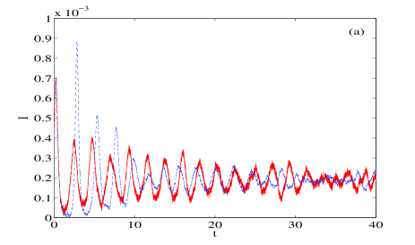
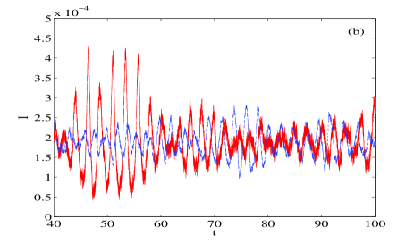
Figure 3: (Color online) Time series of the fraction of the population that is infected with a disease, $I$, computed using the complete, stochastic system of transformed equations of the SEIR model [Eqs. (20a)-(20c)] (red, solid line), and computed using the reduced system of equations of the SEIR model that is based on the deterministic center manifold with a replacement of the noise terms [Eqs. (22a) and (22b)] (blue, dashed line). The standard deviation of the noise intensity used in the simulation is $\sigma_{i}=0.0005$, $i=4,5,6$. The time series is shown for (a) $t=0$ to $t=40$, and for (b) $t=40$ to $t=100$.

Using the same numerical scheme previously described, we numerically integrate the complete, stochastic system of transformed equations of the SEIR model [Eqs. (20a)-(20c)] along with the reduced system of equations that is based on the deterministic center manifold with a replacement of the noise terms [Eqs. (22a) and (22b)]. The complete system is solved for $U$, $V$, and $W$, while the reduced system is solved for $V$ and $W$. In the latter case, $U$ is computed using the center manifold equation given by Eq. (17). Once the values of $U$, $V$, and $W$ are known, we compute the values of $\bar{S}$, $\bar{E}$, and $\bar{I}$ using the transformation given by Eqs. (7a)-(7c). We shift $\bar{S}$, $\bar{E}$, and $\bar{I}$ respectively by $S_{0}$, $E_{0}$, and $I_{0}$ to find the values of $S$, $E$, and $I$.

Figures 3(a)-(b) compares the time series of the fraction of the population that is infected with a disease, $I$, computed using the complete, stochastic system of transformed equations of the SEIR model [Eqs. (20a)-(20c)] with the time series of $I$ computed using the reduced system of equations of the SEIR model that is based on the deterministic center manifold with a replacement of the noise terms [Eqs. (22a) and (22b)]. Figure 3(a) shows the initial transients, while Fig. 3(b) shows the time series after the transients have decayed. One can see that the solution computed using the reduced system quickly becomes out of phase with the solution of the complete system. Use of this reduced system would lead to an incorrect prediction of the initial disease outbreak. Additionally, the predicted amplitude of the initial outbreak would be incorrect. The poor agreement, both in phase and amplitude, between the two solutions continues for long periods of time as seen in Fig. 3(b). We also have computed the cross-correlation of the two time series shown in Fig. 3(a)-(b) to be approximately 0.34. Since the cross-correlation measures the similarity between the two time series, this low value quantitatively suggests poor agreement between the two solutions.

Using the same systems of transformed equations, we compute $140$ years worth of time series for $500$ realizations. Ignoring the first $40$ years of transient solution, the data is used to create a histogram representing the probability density, $p_{SI}$ of the $S$ and $I$ values. Figure 4(a) shows the histogram associated with the complete, stochastic system of transformed equations, while Fig. 4(b) shows the histogram associated with the reduced system of equations with a replacement of the noise terms. The color-bar values in Figs. 4(a)-(b) have been normalized by $10^{-3}$.

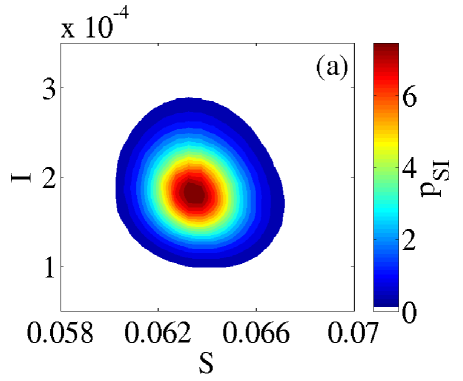
Figure 4: (Color online) Histogram of probability density, $p_{SI}$ of the $S$ and $I$ values found using (a) the complete, stochastic system of transformed equations for the SEIR model [Eqs. (20a)-(20c)], and (b) the reduced system of equations of the SEIR model that is based on the deterministic center manifold with a replacement of the noise terms [Eqs. (22a) and (22b)]. The histograms are created using $100$ years worth of time series (starting with year $40$) for 500 realizations, and the color-bar values have been normalized by $10^{-3}$.

One can see by comparing Fig. 4(a) with Fig. 4(b) that the two probability distributions qualitatively look the same. It also is possible to compare the two distributions using a quantitative measure. The Kullback-Leibler divergence, or relative entropy, measures the difference between the two probability distributions as

$$d_{KL}=\sum\limits_{i,j}P_{i,j}\left|\log{\left(\frac{P_{i,j}}{Q_{i,j}}\right)}\right|,$$ (23)

where $P_{i,j}$ refers to the $(i,j)$th component of the probability density found using the complete, stochastic system of transformed equations [Fig. 4(a)], and $Q_{i,j}$ refers to the $(i,j)$th component of the probability density found using the reduced system of equations [Fig. 4(b)]. In our numerical computation of the relative entropy, we have added $10^{-10}$ to each $P_{ij}$ and $Q_{ij}$. This eliminates the possibility of having a $Q_{ij}=0$ in the denominator of Eq. (23) and does not have much of an effect on the relative entropy.

If the two histograms were identical, then the relative entropy given by Eq. (23) would be $d_{KL}=0$. The two histograms shown in Figs. 4(a)-(b) have a relative entropy of $d_{KL}=0.0391$, which means that the two histograms, while not identical, are quantitatively very similar. However, one cannot rely entirely on the histograms alone to say that the solutions of the complete system and the reduced system agree. As we have seen in Figs. 3(a)-(b), the two solutions have differing amplitudes and are out of phase with one another. It is important to note that these features are not picked up by the histograms of Fig. 4.

V Correct projection of the noise onto the stochastic center manifold

To project the noise correctly onto the center manifold, we will derive a normal form coordinate transform for the complete, stochastic system of transformed equations of the SEIR model given by Eqs. (20a)-(20c). The particular method we use to construct the normal form coordinate transform not only reduces the dimension of the dynamics, but also separates all of the fast processes from all of the slow processes rob08 . This technique has been modified and applied to the large fluctuations of multiscale problems forsch09 .

Many publications knowie83 ; coelti85 ; nam90 ; namlin91 discuss the simplification of a stochastic dynamical system using a stochastic normal form transformation. In some of this work coelti85 ; namlin91 , anticipative noise processes appeared in the normal form transformations, but these integrals of the noise process into the future were not dealt with rigorously.

Later, the rigorous, theoretical analysis needed to support normal form coordinate transforms was developed in Refs. arnimk98, ; arn98, . The technical problem of the anticipative noise integrals also was dealt with rigorously in this work. Even later, another stochastic normal form transformation was developed rob08 . This new method allows for the “[removal of] anticipation … from the slow modes with the result that no anticipation is required after the fast transients decay”(Ref. rob08, , pp. 13). The removal of anticipation leads to a simplification of the normal form. Nonetheless, this simpler normal form retains its accuracy with the original stochastic system rob08 .

We shall use the method of Ref. rob08, to simplify our stochastic dynamical system to one that emulates the long-term dynamics of the original system. The method involves five principles, which we recapitulate here for completeness:

1. Avoid unbounded, secular terms in both the transformation and the evolution equations to ensure a uniform asymptotic approximation.

2. Decouple all of the slow processes from the fast processes to ensure a valid long-term model.

3. Insist that the stochastic slow manifold is precisely the transformed fast processes coordinate being equal to zero.

4. To simplify matters, eliminate as many as possible of the terms in the evolution equations.

5. Try to remove all fast processes from the slow processes by avoiding as much as possible the fast time memory integrals in the evolution equations.

In practice, the original stochastic system of equations (which satisfies the necessary spectral requirements) in $\left(U,V,W\right)^{T}$ coordinates is transformed to a new $\left(Y,X_{1},X_{2}\right)^{T}$ coordinate system using a near-identity stochastic coordinate transform given as

$$U= Y+\xi\left(Y,X_{1},X_{2},\tau\right),$$ (24a)

$$V= X_{1}+\eta\left(Y,X_{1},X_{2},\tau\right),$$ (24b)

$$W= X_{2}+\rho\left(Y,X_{1},X_{2},\tau\right),$$ (24c)

where the specific form of $\xi\left(Y,X_{1},X_{2},\tau\right)$, $\eta\left(Y,X_{1},X_{2},\tau\right)$, and $\rho\left(Y,X_{1},X_{2},\tau\right)$ is chosen to simplify the original system according to the five principles listed previously, and is found using an iterative procedure. To outline the procedure, we provide details for a simple example in Appendix A.

Several iterations lead to coordinate transforms for $U$, $V$, and $W$ along with evolution equations describing the $Y$-dynamics, $X_{1}$-dynamics, and $X_{2}$-dynamics in the new coordinate system. The $Y$-dynamics have exponential decay to the $Y=0$ slow manifold. Substitution of $Y=0$ leads to the coordinate transforms

$$U= \sigma_{4}{\cal G}\left(\phi_{4}\right)+{\frac{{\gamma_{0}}^{2}\left(\sigma_{6}{\cal G}\left(\phi_{6}\right)-X_{2}\right)}{\left(\alpha_{0}+\gamma_{0}\right)^{2}}}+\mu\left[{\frac{\gamma_{0}\beta\left[\sigma_{5}X_{2}{\cal G}\left(\phi_{5}\right)-X_{1}X_{2}+\sigma_{6}X_{1}{\cal G}\left(\phi_{6}\right)\right]}{\left(\alpha_{0}+\gamma_{0}\right)^{2}}}-\right.$$

$$\left.\frac{\sigma_{4}\alpha_{0}\beta\gamma_{0}{\cal G}^{2}\left(\phi_{4}\right)\left[(\alpha_{0}+\gamma_{0})X_{1}+\gamma_{0}X_{2}\right]}{(\alpha_{0}+\gamma_{0})\left(\gamma_{0}+\mu^{2}\right)\left(\alpha_{0}+\mu^{2}\right)}\right]+\mu^{2}\left[{\frac{\gamma_{0}\left[X_{1}\alpha_{0}-2X_{2}+2\sigma_{6}{\cal G}\left(\phi_{6}\right)\right]}{\alpha_{0}\left(\alpha_{0}+\gamma_{0}\right)}}-\right.$$

$$\left.\frac{\sigma_{4}{\cal G}^{2}\left(\phi_{4}\right)}{\left(\gamma_{0}+\mu^{2}\right)\left(\alpha_{0}+\mu^{2}\right)}\left({\frac{2{\gamma_{0}}^{3}+{\alpha_{0}}^{3}}{\alpha_{0}+\gamma_{0}}}+{\frac{{\alpha_{0}}^{2}{\gamma_{0}}^{2}\left(\alpha_{0}+\gamma_{0}\right)}{\left(\gamma_{0}+\mu^{2}\right)\left(\alpha_{0}+\mu^{2}\right)}}\right)-{\frac{\sigma_{5}\gamma_{0}{\cal G}\left(\phi_{5}\right)}{\left(\alpha_{0}+\gamma_{0}\right)^{2}}}\right]+$$

$$\mu^{3}\left[{\frac{\beta\left[-X_{1}+\sigma_{5}{\cal G}\left(\phi_{5}\right)\right]}{\left(\alpha_{0}+\gamma_{0}\right)^{2}}}-\frac{\sigma_{4}\beta{\cal G}^{2}\left(\phi_{4}\right)}{\left(\gamma_{0}+\mu^{2}\right)\left(\alpha_{0}+\mu^{2}\right)}\left({\frac{\alpha_{0}\gamma_{0}}{\alpha_{0}+\gamma_{0}}}+\gamma_{0}X_{2}+X_{1}\left(\alpha_{0}+\gamma_{0}\right)\right)+\right.$$

$$\left.{\frac{\beta\left(\sigma_{6}X_{1}{\cal G}\left(\phi_{6}\right)+\sigma_{5}X_{2}{\cal G}\left(\phi_{5}\right)-X_{1}X_{2}\alpha_{0}\right)}{\alpha_{0}\left(\alpha_{0}+\gamma_{0}\right)}}\right]+\mathcal{O}(\mu^{4}),$$ (25a)

$$V= X_{1}+\mu\left[\frac{\sigma_{4}\alpha_{0}\beta X_{1}{\cal G}(\phi_{4})}{\alpha_{0}+\gamma_{0}}+\frac{\sigma_{4}\alpha_{0}\beta X_{2}{\cal G}(\phi_{4})}{\left(\alpha_{0}+\gamma_{0}\right)^{2}}\right]+\mu^{2}\left[\frac{\sigma_{4}{\cal G}(\phi_{4})\left(\alpha_{0}^{2}+\alpha_{0}\gamma_{0}+\gamma_{0}^{2}\right)}{\gamma_{0}\left(\alpha_{0}+\gamma_{0}\right)^{2}}\right]+$$

$$\mu^{3}\left[\frac{\sigma_{4}\alpha_{0}\beta{\cal G}(\phi_{4})}{\gamma_{0}\left(\alpha_{0}+\gamma_{0}\right)^{2}}+\frac{\sigma_{4}\beta X_{2}{\cal G}(\phi_{4})}{\gamma_{0}\left(\alpha_{0}+\gamma_{0}\right)}+\frac{\sigma_{4}\beta X_{1}{\cal G}(\phi_{4})}{\gamma_{0}^{2}}\right]+\mathcal{O}(\mu^{4}),$$ (25b)

$$W= X_{2}+\mu\left[-\frac{\sigma_{4}\beta X_{1}{\cal G}(\phi_{4})}{\gamma_{0}}-\frac{\sigma_{4}\beta X_{2}{\cal G}(\phi_{4})}{\left(\alpha_{0}+\gamma_{0}\right)}\right]+\mu^{2}\left[\frac{\sigma_{4}{\cal G}(\phi_{4})\left(\alpha_{0}^{2}+\alpha_{0}\gamma_{0}+\gamma_{0}^{2}\right)}{\alpha_{0}\gamma_{0}\left(\alpha_{0}+\gamma_{0}\right)}\right]+$$

$$\mu^{3}\left[-\frac{\sigma_{4}\beta{\cal G}(\phi_{4})}{\gamma_{0}\left(\alpha_{0}+\gamma_{0}\right)}-\frac{\sigma_{4}\left(\alpha_{0}+\gamma_{0}\right)\beta X_{1}{\cal G}(\phi_{4})}{\alpha_{0}\gamma_{0}^{2}}-\frac{\sigma_{4}\beta X_{2}{\cal G}(\phi_{4})}{\alpha_{0}\gamma_{0}}\right]+\mathcal{O}(\mu^{4}),$$ (25c)

where

$${\cal G}(\phi)=e^{-\aleph\tau}*\phi=\int\limits_{-\infty}^{\tau}\exp{[-\aleph\cdot(\tau-s)]\phi(s)}ds,~{}~{}~{}\aleph=\frac{\alpha_{0}\gamma_{0}\left(\alpha_{0}+\gamma_{0}\right)}{\left(\alpha_{0}+\mu^{2}\right)\left(\gamma_{0}+\mu^{2}\right)},$$ (26)

and

$${\cal G}^{2}(\phi)=e^{-\aleph\tau}*e^{-\aleph\tau}*\phi.$$ (27)

All of the stochastic terms in Eqs. (25a)-(25c) consist of integrals of the noise process into the past (convolutions), as given by Eqs. (26) and (27). These memory integrals are fast-time processes. Since we are interested in the long-term slow processes and since the expectation of ${\cal G}$ equals $e^{-\aleph\tau}*E[\phi]$, where $E[\phi]=0$, we neglect the memory integrals and the higher-order multiplicative terms found in Eqs. (25a)-(25c) so that

$$U= -\frac{\gamma_{0}^{2}X_{2}}{\left(\alpha_{0}+\gamma_{0}\right)^{2}}-\frac{\mu\beta X_{1}}{\left(\alpha_{0}+\gamma_{0}\right)}\left(\frac{\mu^{2}}{\left(\alpha_{0}+\gamma_{0}\right)}+\frac{\gamma_{0}X_{2}}{\left(\alpha_{0}+\gamma_{0}\right)}+\mu^{2}X_{2}\right)$$

$$+\frac{\mu^{2}\gamma_{0}}{\left(\alpha_{0}+\gamma_{0}\right)}\left(X_{1}-\frac{2X_{2}}{\alpha_{0}}\right),$$ (28a)

$$V= ~{}X_{1},$$ (28b)

$$W= ~{}X_{2}.$$ (28c)

Note that Eq. (28a) is the deterministic center manifold equation, and at first-order, matches the center manifold equation that was found previously [Eq. (17)].

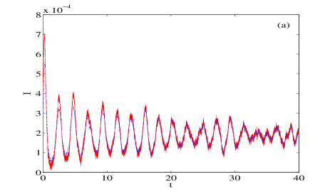
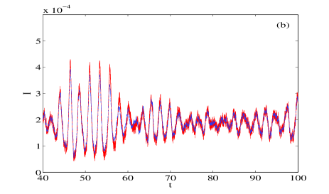
Figure 5: (Color online) Time series of the fraction of the population that is infected with a disease, $I$, computed using the complete, stochastic system of transformed equations of the SEIR model [Eqs. (20a)-(20c)] (red, solid line), and computed using the reduced system of equations of the SEIR model that is found using the stochastic normal form coordinate transform [Eqs. (29a), (29b), (45a), and (45b)] (blue, dashed line). The standard deviation of the noise intensity used in the simulation is $\sigma_{i}=0.0005$, $i=4,5,6$. The time series is shown for (a) $t=0$ to $t=40$, and for (b) $t=40$ to $t=100$.

Substitution of $Y=0$ and neglecting all multiplicative noise terms and memory integrals using the argument from above (so that we consider only first-order noise terms) leads to the following reduced system of evolution equations on the center manifold:

$$\frac{dX_{1}}{d\tau}=F(X_{1}(\tau),X_{2}(\tau)),$$ (29a)

$$\frac{dX_{2}}{d\tau}=G(X_{1}(\tau),X_{2}(\tau)).$$ (29b)

The specific form of $F$ and $G$ in Eqs. (29a) and (29b) are complicated, and are therefore presented in Appendix B.

We numerically integrate the complete, stochastic system of transformed equations of the SEIR model [Eqs. (20a)-(20c)] along with the reduced system of equations that is found using the stochastic normal form coordinate transform [Eqs. (29a), (29b), (45a), and (45b)]. The complete system is solved for $U$, $V$, and $W$, while the reduced system is solved for $X_{1}=V$ and $X_{2}=W$. In the latter case, $U$ is computed using the center manifold equation given by Eq. (28a). As before, once the values of $U$, $V$, and $W$ are known, we compute the values of $\bar{S}$, $\bar{E}$ , and $\bar{I}$ using the transformation given by Eqs. (7a)-(7c). We shift $\bar{S}$, $\bar{E}$, and $\bar{I}$ respectively by $S_{0}$, $E_{0}$, and $I_{0}$ to find the values of $S$, $E$, and $I$.

Figures 5(a)-(b) compares the time series of the fraction of the population that is infected with a disease, $I$, computed using the complete, stochastic system of transformed equations of the SEIR model [Eqs. (20a)-(20c)] with the time series of $I$ computed using the reduced system of equations of the SEIR model that is found using the stochastic normal form coordinate transform [Eqs. (29a), (29b), (45a), and (45b)]. Figure 5(a) shows the initial transients, while Fig. 5(b) shows the time series after the transients have decayed. One can see that there is excellent agreement between the two solutions. The initial outbreak is successfully captured by the reduced system. Furthermore, Fig. 5(b) shows that the reduced system accurately predicts recurrent outbreaks for a time scale that is orders of magnitude longer than the relaxation time. This is not surprising since the solution decays exponentially throughout the transient and then remains close to the lower-dimensional center manifold. Since we are not looking at periodic orbits, there are no secular terms in the asymptotic expansion, and the result is valid for all time. Additionally, any noise drift on the center manifold results in bounded solutions due to sufficient dissipation transverse to the manifold. The cross-correlation of the two time series shown in Fig. 5 is approximately 0.98, which quantitatively suggests there is excellent agreement between the two solutions.

Using the same systems of transformed equations, we compute $140$ years worth of time series for $500$ realizations. As before, we ignore the first $40$ years worth of transient solution, and the data is used to create a histogram representing the probability density, $p_{SI}$ of the $S$ and $I$ values. Figure 6(a) shows the histogram associated with the complete, stochastic system of transformed equations, while Fig. 6(b) shows the histogram associated with the reduced system of equations found using the normal form coordinate transform. The color-bar values in Figs. 6(a)-(b) have been normalized by $10^{-3}$.

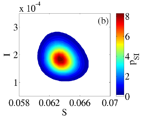
Figure 6: (Color online) Histogram of probability density, $p_{SI}$ of the $S$ and $I$ values found using (a) the complete, stochastic system of transformed equations for the SEIR model with mortality [Eqs. (20a)-(20c)], and (b) the reduced system of equations of the SEIR model with mortality that is found using the stochastic normal form coordinate transform [Eqs. (29a), (29b), (45a), and (45b)]. The histograms are created using $100$ years worth of time series (starting with year $40$) for 500 realizations, and the color-bar values have been normalized by $10^{-3}$.

As we saw with Figs. 4(a)-(b), the probability distribution shown in Fig. 6(a) looks qualitatively the same as the probability distribution shown in Fig. 6(b). Using the Kullback-Leibler divergence given by Eq. (23), we have found that the two histograms shown in Figs. 6(a)-(b) have a relative entropy of $d_{KL}=0.0953$. Since this value is close to zero, the two histograms are quantitatively very similar.

In addition to computing the cross-correlation between the solution of the original system and the solutions of the two reduced systems for $\sigma_{i}=0.0005$, we have computed the cross-correlation for the case of zero noise as well as for noise intensities ranging from $\sigma=5.0\times 10^{-10}$ to $\sigma=5.0\times 10^{-5}$. These cross-correlations were computed using time series from $t=800$ to $t=1000$. For the deterministic case (zero noise), the cross-correlation between the time series which were computed using the original system and the reduced system based on the deterministic center manifold is $1.0$, since the agreement is perfect. The cross-correlation between the original system and the reduced system found using the stochastic normal form is also $1.0$. Figure 7 shows the cross-correlation between the original system and the two reduced systems for various values of $\sigma$.

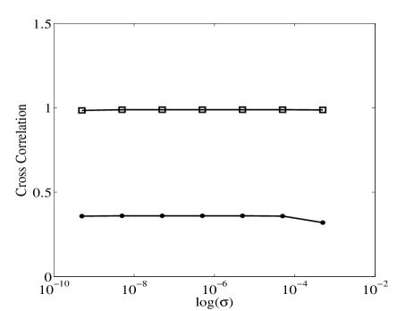
Figure 7: Cross-correlation between time series found using the original, stochastic system of transformed equations and the reduced system of equations based on the deterministic center manifold (“circle” markers), and cross-correlation between time series found using the original, stochastic system of transformed equations and the reduced system of equations based on the stochastic normal form coordinate transform (“square” markers). The cross-correlation is computed using time series from $t=800$ to $t=1000$.

One can see in Fig. 7 that the solutions found using the reduced system based on the deterministic center manifold compare poorly with the original system at very low noise values. Furthermore, as the noise increases, the agreement between the two solutions gets worse. On the other hand, Fig. 7 shows that the solutions computed using the reduced system found using the normal form coordinate transform compare very well with the solutions to the original system across a wide range of small noise intensities.

VI Discussion

We have demonstrated that the normal form coordinate transform method reduces the Langevin system so that both the noise and dynamics are accurately projected onto the lower-dimensional manifold. It is natural to consider (a) the replacement of the stochastic term by a deterministic, period drive of small amplitude, and (b) the extension to finite populations. These cases are discussed respectively in Sec. VI.1 and Sec. VI.2.

VI.1 The Case of Deterministic Forcing

A single time series realization of the noise might be thought of as a deterministic function of small amplitude driving the system. One could rederive the normal form for such a deterministic function. However, since our derived  normal form holds specifically for the case of white noise,  we show that a simple replacement of the stochastic realization with a deterministic realization does not work. As an example, one could consider the following sinusoidal functions:

$$\sigma_{1}\phi_{1}=\cos{(10\pi\mu t)}/8000,$$ (30a)

$$\sigma_{2}\phi_{2}=\sin{(4\pi\mu t)}/8000,$$ (30b)

$$\sigma_{3}\phi_{3}=\cos{(10\pi\mu t)}/8000,$$ (30c)

where $\sigma_{4}\phi_{4}$, $\sigma_{5}\phi_{5}$, and $\sigma_{6}\phi_{6}$ are given by Eqs. (21a)-(21c). Using Eqs. (30a)-(30c) or some other similar deterministic drive, the solution computed using the reduced system based on the deterministic center manifold analysis will agree perfectly with the solution computed using the complete system of equations. On the other hand, since the reduced system based on the normal form analysis was derived specifically for white noise, the transient solution found using this reduced system will not agree with the solution found using the complete system. It is possible to find a normal form coordinate transform for periodic forcing, but the normal form will be different than the one derived in this article for white noise.

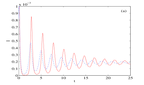
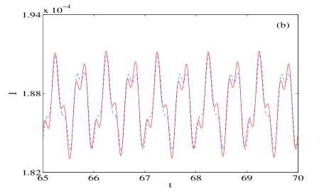
Figure 8: (Color online) Time series of the fraction of the population that is infected with a disease, $I$, computed using the complete system of transformed equations of the SEIR model [Eqs. (20a)-(20c)] (red, solid line), and computed using the reduced system of equations of the SEIR model that is found using the normal form coordinate transform [Eqs. (29a), (29b), (45a), and (45b)] (blue, dashed line). The stochastic terms in both systems have been replaced by the deterministic terms given by Eqs. (30a)-(30b). The time series is shown from (a) $t=0$ to $t=25$, and from (b) $t=65$ to $t=70$.

Figures 8(a)-(b) compares the time series of the fraction of the population that is infected with a disease, $I$, computed using the complete system of transformed equations of the SEIR model [Eqs. (20a)-(20c)] with the time series of $I$ computed using the reduced system of equations of the SEIR model that is found using the stochastic normal form coordinate transform [Eqs. (29a), (29b), (45a), and (45b)], but where the stochastic terms of both systems have been replaced by the deterministic terms given by Eqs. (30a)-(30c). Figure 8(a) shows the initial transients, while Fig. 8(b) shows a piece of the time series after the transients have decayed. One can see in Figs. 8(a)-(b) that although the two solutions eventually become relatively synchronized with one another, there is poor agreement, both in phase and amplitude, throughout the transient.

VI.2 The Case of Finite Populations

The solutions to the original system and both reduced systems are continuous solutions based on an infinite population assumption, and are found using Langevin equations having Gaussian noise. It is interesting to examine the effects of general noise by using a Markov simulation to compare solutions of the original and reduced systems.

The complete system in the original variables (see page 5) will evolve in time $t$ in the following way:

$$\begin{array}[]{lcl}\mbox{transition}&&\mbox{rate}\\ (s-1,e+1,i)&&\beta si/N\\ (s,e-1,i+1)&&\alpha e\\ (s,e,i-1)&&\gamma i\\ (s+1,e,i)&&\mu N\\ (s-1,e,i)&&\mu s\\ (s,e-1,i)&&\mu e\\ (s,e,i-1)&&\mu i\end{array}.$$ (31)

Using a total population size of $N=10$ million, we have performed a Markov simulation of the system. After completing the Markov simulation, we divided $s$, $e$, and $i$ by $N$ to find $S$, $E$, and $I$. Figure 9(a) shows a time series, after the transients have decayed, of the fraction of the population that is infected with a disease, $I$. The results reflect both the mean and the frequency of the deterministic system. Performing the simulation for $500$ realizations allows us to create a histogram representing the probability density, $p_{SI}$ of the $S$ and $I$ values. This histogram is shown in Fig. 9(b), and one can see that the probability density reflects the amplitude, which varies with the population size, of $S$ and $I$. The color-bar values in Fig. 9(b) have been normalized by $10^{-4}$

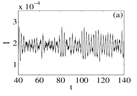
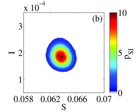
Figure 9: (a) Time series of the fraction of the population that is infected with a disease, $I$, computed using a Markov simulation of the complete, original equations of the SEIR model [Eq. (31)], and (b) (color online) a histogram of probability density, $p_{SI}$ of the $S$ and $I$ values found using a Markov simulation of Eq. (31). The histogram is created using $100$ years worth of data (starting with year $40$) for 500 realizations, and the color-bar values have been normalized by $10^{-4}$.

The complete system in the transformed variables has the stable endemic equilibrium at the origin. To bound the dynamics to the first octant, we use the fact that $s\geq 0$, $e\geq 0$, and $i\geq 0$ to derive the appropriate inequalities for the transformed, discrete variables $u$, $v$, and $w$. These inequalities can be found in Appendix C as Eq. (46). These inequalities enable us to define new discrete variables $Y_{1}$, $Y_{2}$, and $Y_{3}$, given by Eqs. (47a)-(47c) in Appendix C.

In the $Y_{i}$ variables, we define evolution relationships similar to those found in Eq. (31). The complete transformed system will evolve in time $\tau$ according to the transition and rates given by Eq. (48) in Appendix C.

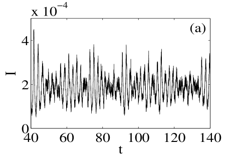
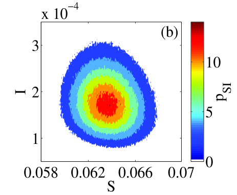
Figure 10: (a) Time series of the fraction of the population that is infected with a disease, $I$, computed using a Markov simulation of the complete, transformed equations of the SEIR model [Eq. (48)], and (b) (color online) a histogram of probability density, $p_{SI}$ of the $S$ and $I$ values found using a Markov simulation of Eq. (48). The histogram is created using $100$ years worth of data (starting with year $40$) for 500 realizations, and the color-bar values have been normalized by $10^{-4}$.

After performing a Markov simulation of Eq. (48) with a population size of $N=10$ million, we can compare the dynamics of the transformed system to the dynamics of the original system by transforming the $Y_{i}$ variables in the time series back to the original $s$, $e$, and $i$ variables. Dividing by $N$ yields $S$, $E$, and $I$. Figure 10(a) shows a time series, after the transients have decayed, of the fraction of the population that is infected with a disease, $I$. The mean and the frequency agree with those found from the Markov simulation of the original system. We have performed the simulation for $500$ realizations, and a histogram representing the probability density, $p_{SI}$ is shown in Fig. 10(b). The color-bar values in Fig. 10(b) have been normalized by $10^{-4}$. One can see in Fig. 10(a) that the relative fluctuations of the $I$ component has nearly doubled. While the fluctuation size was 0.152 for the original system, it is 0.310 for the transformed system. Additionally, the two histograms shown in Figs. 9(b) and 10(b) have a relative entropy of $d_{KL}=0.9519$, which means they are not in agreement. Because the simulation of the stochastic dynamics in the complete system of transformed variables do not qualitatively (or quantitatively) resemble the original stochastic system, we cannot expect that the reduced system will agree with either the original or the transformed systems. Therefore, much care should be exercised when extending the model reduction results (which show outstanding agreement) derived for a specific type of noise in the limit of infinite population to finite populations with a more general type of noise.

VII Conclusions

We have considered the dynamics of an SEIR epidemiological model with stochastic forcing in the form of additive, Gaussian noise. We have presented two methods of model reduction, whereby the goal is to project both the noise and the dynamics onto the stochastic center manifold. The first method uses the deterministic center manifold found by neglecting the stochastic terms in the governing equations, while the second method uses a stochastic normal form coordinate transform.

Since the original system of governing equations does not have the necessary spectral structure to employ either deterministic or stochastic center manifold theory, the system of equations has been transformed using an appropriate linear transformation coupled with appropriate parameter scaling. At this stage, the first method of model reduction can be performed by computing the deterministic center manifold equation. Substitution of this equation into the complete, stochastic system of transformed equations leads to a reduced system of stochastic evolution equations.

The solutions of the complete, stochastic system of transformed equations as well as the reduced system of equations were computed numerically. We have shown that the individual time series do not agree, because the noise has not been correctly projected onto the stochastic center manifold. However, by comparing histograms of the probability density, $p_{SI}$ of the $S$ and $I$ values, we saw that there was very good agreement. This is caused by the fact that although the two solutions are out of phase with one another, their range of amplitude values are similar. The phase difference is not represented in the two histograms. This is a real drawback when trying to predict the timing of outbreaks, and leads to potential problems when considering epidemic control, such as the enhancement of disease extinction through random vaccine control dyscla08 .

To accurately project the noise onto the manifold, we derived a stochastic normal form coordinate transform for the complete, stochastic system of transformed equations. The numerical solution to this reduced system was compared with the solution to the original system, and we showed that there was excellent agreement, both qualitatively and quantitatively. As with the first method, the histograms of the probability density, $p_{SI}$ of the $S$ and $I$ values agree very well.

It should be noted that the use of these two reduction methods is not constrained to problems in epidemiology, but rather may be used for many types of physical problems. For some generic systems, such as the singularly perturbed, damped Duffing oscillator, either reduction method can be used since the terms in the normal form coordinate transform which lead to the average stochastic center manifold being different from the deterministic center manifold occur at very high order forsch09 . In other words, the average stochastic center manifold and deterministic center manifold are virtually identical. For the SEIR model considered in this article, there are terms at low order in the normal form transform which cause a significant difference between the average stochastic center manifold and the deterministic manifold. Therefore, as we have demonstrated, when working with the SEIR model, one must use the normal form coordinate transform method to correctly project the noise onto the center manifold.

In summary, we have presented a new method of stochastic model reduction that allows for impressive improvement in time series prediction. The reduced model captures both the amplitude and phase accurately for a temporal scale that is many orders of magnitude longer than the typical relaxation time. Since sufficient statistics of disease data are limited due to short time series collection, the results presented here provide a potential method to properly model real, stochastic disease data in the time domain. Such long-term accuracy of the reduced model will allow for the application of effective control of a disease where phase differences between outbreak times and vaccine controls are important. Additionally, since our method is general, it may be applied to very high-dimensional epidemic models, such as those involving adaptive networks. From a dynamical systems viewpoint, the reduction method has the potential to accurately capture new, emergent dynamics as we increase the size of the random fluctuations. This could be a means to identify new noise-induced phenomena in generic stochastic systems.

Appendix A Details of the Iterative Procedure for a Simple Example

We consider the system given by

$$\frac{dx}{d\tau}= \mu(y+\sigma\phi),$$ (32a)

$$\frac{dy}{d\tau}= x-x^{3}-y,$$ (32b)

$$\frac{d\mu}{d\tau}= 0.$$ (32c)

The iterative procedure begins by letting

$$x\approx X,$$ (33a)

$$X^{\prime}\approx 0,$$ (33b)

and by finding a change to the $y$ coordinate (fast process) with the form

$$y=Y+\eta(\tau,X,Y)+\ldots,$$ (34a)

$$Y^{\prime}=-Y+G(\tau,X,Y)+\ldots,$$ (34b)

where $\eta$ and $G$ are small corrections to the coordinate transform and the corresponding evolution equation. Substitution of Eqs. (33a)-(34b) into Eq. (32b) gives the equation

$$Y^{\prime}+\frac{\partial\eta}{\partial\tau}+\frac{\partial\eta}{\partial X}\frac{\partial X}{\partial\tau}+\frac{\partial\eta}{\partial Y}\frac{\partial Y}{\partial\tau}=-Y-\eta+X-X^{3}.$$ (35)

Replacing $Y^{\prime}=\partial Y/\partial\tau$ with $-Y+G$ [Eq. (34b)], noting that $\partial X/\partial\tau=0$ [Eq. (33b)], and ignoring the term $\partial\eta/\partial Y\cdot G$ since it is a product of small corrections leads to

$$G+\frac{\partial\eta}{\partial\tau}-Y\frac{\partial\eta}{\partial Y}+\eta=X-X^{3}.$$ (36)

Equation (36) must now be solved for $G$ and $\eta$. In order to keep the evolution equation [Eq. (34b)] as simple as possible (principle (4) of Sec. V), we let $G=0$, which means that the coordinate transform [Eq. (34a)] is modified by $\eta=X-X^{3}$. Therefore, the new approximation of the coordinate transform and its dynamics are given by

$$y=Y+X-X^{3}+\mathcal{O}(\zeta^{2}),$$ (37a)

$$Y^{\prime}=-Y+\mathcal{O}(\zeta^{2}),$$ (37b)

where $\zeta=|(X,Y,\mu,\sigma)|$ so that $\zeta$ provides a count of the number of $X$, $Y$, $\mu$, and $\sigma$ factors in any one term.

For the second iteration, we seek a correction to the $x$ coordinate (slow process) with the form

$$x=X+\xi(\tau,X,Y)+\ldots,$$ (38a)

$$X^{\prime}=F(\tau,X,Y)+\ldots,$$ (38b)

where $\xi$ and $F$ are small corrections. Substitution of Eqs. (37a)-(38b) into Eq. (32a) leads to

$$X^{\prime}+\frac{\partial\xi}{\partial\tau}+\frac{\partial\xi}{\partial X}\frac{\partial X}{\partial\tau}+\frac{\partial\xi}{\partial Y}\frac{\partial Y}{\partial\tau}=\mu(Y+X-X^{3})+\mu\sigma\phi.$$ (39)

Replacing $X^{\prime}=\partial X/\partial\tau$ with $F$ [Eq. (38b)], replacing $\partial Y/\partial\tau$ with $-Y$ [Eq. (37b)], and ignoring the term $\partial\xi/\partial X\cdot F$ since it is a product of small corrections gives the equation:

$$F+\frac{\partial\xi}{\partial\tau}-Y\frac{\partial\xi}{\partial Y}=\mu(Y+X-X^{3})+\mu\sigma\phi.$$ (40)

Equation (40) must now be solved for $F$ and $\xi$. As in the first step, we employ principle (4) and keep the evolution equation [Eq. (38b)] as simple as possible. However, since the terms $\mu(X-X^{3})$ located on the right-hand side of Eq. (40) do not contain $\tau$ or $Y$, these terms must be included in F. Therefore, one piece of $F$ will be $F=\mu(X-X^{3})$.

The remaining deterministic term on the right-hand side of Eq. (40) contains $Y$. This term can therefore be integrated into $\xi$. The equation to be solved is

$$-Y\frac{\partial\xi}{\partial Y}=\mu Y,$$ (41)

whose solution is given as $\xi=-\mu Y$.

To abide by principle (4), we would like to integrate the stochastic piece on the right-hand side of Eq. (40) into $\xi$, by solving the equation

$$\partial\xi/\partial\tau=\mu\sigma\phi.$$ (42)

However, the solution of Eq. (42) is given by

$$\xi=\mu\sigma\int\phi\,d\tau,$$ (43)

which has secular growth like a Wiener process. Since this would violate principle (1), we must let $F=\mu\sigma\phi$.

Putting the three pieces together yields $\xi=-\mu Y$ and $F=\mu(X-X^{3})+\mu\sigma\phi$. Therefore, the new approximation of the coordinate transform and its dynamics are given by

$$x=X-\mu Y+\mathcal{O}(\zeta^{3}),$$ (44a)

$$X^{\prime}=\mu(X-X^{3})+\mu\sigma\phi+\mathcal{O}(\zeta^{3}).$$ (44b)

The construction of the normal form continues by seeking corrections, $\xi$ and $F$, to the $x$ coordinate transform and the $X$ evolution using the updated residual of the $x$ equation [Eq. (32a)], and by seeking corrections, $\eta$ and $G$, to the $y$ coordinate transform and the $Y$ evolution equation using the updated residual of the $y$ equation [Eq. (32b)].

Appendix B Reduced, stochastic SEIR model: Correct projection of the noise

The specific form of $F$ and $G$ in Eqs. (29a) and (29b) are given as

$$F= -\left[\alpha_{0}^{2}\gamma_{0}^{3}X_{2}+\frac{\mu\beta\alpha_{0}^{2}}{\left(\alpha_{0}+\gamma_{0}\right)}\gamma_{0}^{2}\left(-\frac{\gamma_{0}^{2}}{\alpha_{0}+\gamma_{0}}X_{2}^{2}+\alpha_{0}X_{1}X_{2}\right)+\mu^{2}\left(\alpha_{0}\gamma_{0}^{3}X_{1}+\right.\right.$$

$$\left.\frac{\alpha_{0}\gamma_{0}^{2}\left(2\alpha_{0}^{3}+5\alpha_{0}^{2}\gamma_{0}+5\alpha_{0}\gamma_{0}^{2}+\gamma_{0}^{3}\right)}{\left(\alpha_{0}+\gamma_{0}\right)^{2}}X_{2}-\frac{\alpha_{0}^{2}\beta^{2}\gamma_{0}^{2}}{\left(\alpha_{0}+\gamma_{0}\right)}X_{1}^{2}X_{2}-\frac{\alpha_{0}^{2}\beta^{2}\gamma_{0}^{3}}{\left(\alpha_{0}+\gamma_{0}\right)^{2}}X_{1}X_{2}^{2}\right)+$$

$$\mu^{3}\left(\alpha_{0}^{2}\beta\gamma_{0}X_{1}-\frac{\alpha_{0}^{2}\beta\gamma_{0}^{3}}{\left(\alpha_{0}+\gamma_{0}\right)^{2}}X_{2}+\frac{\alpha_{0}^{2}\beta\gamma_{0}^{2}}{\left(\alpha_{0}+\gamma_{0}\right)}X_{1}^{2}-\frac{3\alpha_{0}\beta\gamma_{0}^{3}}{\left(\alpha_{0}+\gamma_{0}\right)}X_{2}^{2}+\right.$$

$$\left.\left.\frac{\alpha_{0}\beta\gamma_{0}\left(\alpha_{0}^{3}-\alpha_{0}^{2}\gamma_{0}-3\alpha_{0}\gamma_{0}^{2}-3\gamma_{0}^{3}\right)}{\left(\alpha_{0}+\gamma_{0}\right)^{2}}X_{1}X_{2}\right)\right]/\left[\gamma_{0}\left(\alpha_{0}+\gamma_{0}\right)\left(\alpha_{0}+\mu^{2}\right)\left(\gamma_{0}+\mu^{2}\right)\right]+$$

$$\sigma_{5}\phi_{5}-\frac{\mu^{2}(\alpha_{0}^{2}+\alpha_{0}\gamma_{0}+\gamma_{0}^{2})}{(\alpha_{0}+\gamma_{0})^{3}}\left(\frac{\sigma_{4}\alpha_{0}\phi_{4}}{\gamma_{0}}+\frac{\sigma_{6}\gamma_{0}\phi_{6}}{\alpha_{0}+\gamma_{0}}\right)-$$

$$\frac{\mu^{3}\alpha_{0}\beta}{(\alpha_{0}+\gamma_{0})^{3}}\left(\frac{\sigma_{4}\alpha_{0}\phi_{4}}{\gamma_{0}}+\frac{\sigma_{6}\gamma_{0}\phi_{6}}{(\alpha_{0}+\gamma_{0})}\right),$$ (45a)

$$G= \left[\mu\left(\frac{\alpha_{0}^{3}\beta\gamma_{0}^{2}}{\left(\alpha_{0}+\gamma_{0}\right)}X_{1}X_{2}-\frac{\alpha_{0}^{2}\beta\gamma_{0}^{4}}{\left(\alpha_{0}+\gamma_{0}\right)^{2}}X_{2}^{2}\right)+\mu^{2}\left(-\alpha_{0}^{2}\gamma_{0}^{2}X_{1}+\frac{\alpha_{0}^{2}\gamma_{0}^{4}}{\left(\alpha_{0}+\gamma_{0}\right)^{2}}X_{2}-\right.\right.$$

$$\left.\frac{\alpha_{0}^{2}\beta^{2}\gamma_{0}^{2}}{\left(\alpha_{0}+\gamma_{0}\right)}X_{1}^{2}X_{2}-\right.\left.\frac{\alpha_{0}^{2}\beta^{2}\gamma_{0}^{3}}{\left(\alpha_{0}+\gamma_{0}\right)^{2}}X_{1}X_{2}^{2}\right)+\mu^{3}\left(\alpha_{0}^{2}\beta\gamma_{0}X_{1}-\frac{\alpha_{0}^{2}\beta\gamma_{0}^{3}}{\left(\alpha_{0}+\gamma_{0}\right)^{2}}X_{2}+\right.$$

$$\left.\frac{\alpha_{0}^{2}\beta\gamma_{0}^{2}\left(\alpha_{0}+\mu^{2}\right)\left(\gamma_{0}+\mu^{2}\right)}{\left(\alpha_{0}+\gamma_{0}\right)}X_{1}^{2}-\frac{3\alpha_{0}\beta\gamma_{0}^{3}}{\left(\alpha_{0}+\gamma_{0}\right)}X_{2}^{2}-3\alpha_{0}\beta\gamma_{0}^{2}\left(\alpha_{0}+\mu^{2}\right)\left(\gamma_{0}+\mu^{2}\right)X_{1}X_{2}+\right.$$

$$\left.\left.\frac{\alpha_{0}^{2}\beta\gamma_{0}\left(\alpha_{0}^{2}+2\alpha_{0}\gamma_{0}+3\gamma_{0}^{2}\right)}{\left(\alpha_{0}+\gamma_{0}\right)^{2}}X_{1}X_{2}\right)\right]/\left[\alpha_{0}\gamma_{0}\left(\alpha_{0}+\mu^{2}\right)\left(\gamma_{0}+\mu^{2}\right)\right]+\sigma_{6}\phi_{6}+$$

$$\frac{\mu^{2}\sigma_{4}\left(\alpha_{0}^{2}+\alpha_{0}\gamma_{0}+\gamma_{0}^{2}\right)}{\alpha_{0}\gamma_{0}\left(\alpha_{0}+\gamma_{0}\right)}\phi_{4}+\frac{\mu^{2}\sigma_{6}\left[\gamma_{0}^{3}\left(\alpha_{0}+\mu^{2}\right)\left(\gamma_{0}+\mu^{2}\right)+\alpha_{0}\gamma_{0}\left(\alpha_{0}+\gamma_{0}\right)\right]}{\alpha_{0}\left(\alpha_{0}+\gamma_{0}\right)^{3}}\phi_{6}+$$

$$\frac{\mu^{3}\beta}{\left(\alpha_{0}+\gamma_{0}\right)}\left(\frac{\sigma_{4}\phi_{4}}{\gamma_{0}}+\frac{\sigma_{6}\gamma_{0}\phi_{6}}{\left(\alpha_{0}+\gamma_{0}\right)^{2}}\right).$$ (45b)

Appendix C Markov simulation for transformed SEIR model

The complete system in the transformed variables has the stable endemic equilibrium at the origin. To bound the dynamics to the first octant, we transform the new variables by using the original properties of $s\geq 0$, $e\geq 0$, and $i\geq 0$, so that

$$u\leq{\frac{\mu^{2}N\gamma_{0}}{\alpha_{0}\left(\alpha_{0}+\gamma_{0}\right)}},~{}~{}~{}-{\frac{N\gamma_{0}\left(\beta{\mu}^{3}+{\alpha_{0}}^{2}+\gamma_{0}\alpha_{0}\right)}{\alpha_{0}\beta\mu\left(\alpha_{0}+\gamma_{0}\right)}}\leq v,~{}~{}~{}-{\frac{N\mu^{2}\left(\alpha_{0}+\gamma_{0}\right)}{\gamma_{0}\alpha_{0}}}\leq w.$$ (46)

Therefore, we define the following new variables:

$$Y_{1} = -u+{\frac{N\mu^{2}\gamma_{0}}{\alpha_{0}\left(\alpha_{0}+\gamma_{0}\right)}},$$ (47a)

$$Y_{2} = v+{\frac{N\gamma_{0}\left(\beta{\mu}^{3}+{\alpha_{0}}^{2}+\gamma_{0}\alpha_{0}\right)}{\alpha_{0}\beta\mu\left(\alpha_{0}+\gamma_{0}\right)}},$$ (47b)

$$Y_{3} = w+{\frac{N\mu^{2}\left({\it\alpha_{0}}+\gamma_{0}\right)}{\gamma_{0}\alpha_{0}}}.$$ (47c)

In these variables, we define evolution relationships similar to Eq. (31). The complete transformed system will evolve in $\tau$ the following way:

$$\begin{array}[]{lcl}\mbox{transition}&&\mbox{rate}\\ (Y_{1}+1,Y_{2},Y_{3})&&\frac{\beta\mu}{N}\left(\frac{\gamma_{0}}{\alpha_{0}+\gamma_{0}}Y_{2}Y_{3}+Y_{1}^{2}\right)\\ (Y_{1}-1,Y_{2},Y_{3})&&(\alpha_{0}+\mu^{2})Y_{1}+\frac{\beta\mu}{N}\left(\frac{\gamma_{0}}{\alpha_{0}+\gamma_{0}}Y_{1}Y_{3}+Y_{1}Y_{2}\right)\\ (Y_{1},Y_{2}+1,Y_{3})&&\mu^{2}N+\frac{\beta\mu}{N}\left({\frac{\alpha_{0}}{\left(\alpha_{0}+\gamma_{0}\right)}Y_{1}Y_{3}}+{\frac{\alpha_{0}}{\gamma_{0}}}Y_{1}Y_{2}\right)\\ (Y_{1},Y_{2}-1,Y_{3})&&\alpha_{0}Y_{1}+\mu^{2}Y_{2}+\frac{\beta\mu}{N}\left({\frac{\alpha_{0}}{\left(\alpha_{0}+\gamma_{0}\right)}}Y_{2}Y_{3}+{\frac{\alpha_{0}}{\gamma_{0}}}{Y_{1}}^{2}\right)\\ (Y_{1},Y_{2},Y_{3}+1)&&(\alpha_{0}+\gamma_{0})Y_{1}+\frac{\beta\mu}{N}\left(Y_{2}Y_{3}+{\frac{\left(\alpha_{0}+\gamma_{0}\right)}{\gamma_{0}}}{Y_{1}}^{2}\right)\\ (Y_{1},Y_{2},Y_{3}-1)&&(\gamma_{0}+\mu^{2})Y_{3}+\frac{\beta\mu}{N}\left(Y_{1}Y_{3}+{\frac{\left(\alpha_{0}+\gamma_{0}\right)}{\gamma_{0}}}Y_{1}Y_{2}\right)\end{array}.$$ (48)

References

- (1) R. M. Anderson and R. M. May, Infectious Diseases of Humans (Oxford University Press, 1991).
- (2) N. T. J. Bailey, The Mathematical Theory of Infectious Diseases (Charles Griffin, London, 1975).
- (3) G. Marion, E. Renshaw, and G. Gibson, “Stochastic modelling of environmental variation for biological populations,” Theor. Popul. Biol. 57, 197 (2000).
- (4) H. T. H. Nguyen and P. Rohani, “Noise, nonlinearity and seasonality: The epidemics of whooping cough revisited,” J. Roy. Soc. Interface 5, 403 (2008).
- (5) P. Rohani, M. J. Keeling, and B. T. Grenfell, “The interplay between determinism and stochasticity in childhood diseases,” Am. Nat. 159, 469 (2002).
- (6) D. A. Rand and H. B. Wilson, “Chaotic stochasticity - A ubiquitous source of unpredictability in epidemics,” P. Roy. Soc. B - Biol. Sci. 246, 179 (1991).
- (7) L. Billings, E. M. Bollt, and I. B. Schwartz, “Phase-space transport of stochastic chaos in population dynamics of virus spread,” Phys. Rev. Lett. 88, 234101 (2002).
- (8) L. Stone, R. Olinky, and A. Huppert, “Seasonal dynamics of recurrent epidemics,” Nature 446, 533 (2007).
- (9) I. B. Schwartz, L. Billings, and E. M. Bollt, “Dynamical epidemic suppression using stochastic prediction and control,” Phys. Rev. E 70, 046220 (2004).
- (10) R. Pastor-Satorras and A. Vespignani, “Epidemic dynamics and endemic states in complex networks,” Phys. Rev. E 63, 066117 (2001).
- (11) Y. Moreno, R. Pastor-Satorras, and A. Vespignani, “Epidemic outbreaks in complex heterogeneous networks,” Eur. Phys. J. B 26, 521 (2002).
- (12) A. Vazquez, “Spreading dynamics on small-world networks with connectivity fluctuations and correlations,” Phys. Rev. E 74, 056101 (2006).
- (13) D. J. Watts, R. Muhamad, D. C. Medina, and P. S. Dodds, “Multiscale, resurgent epidemics in a hierarchical metapopulation model,” P. Natl. Acad. Sci. USA 102, 11157 (2005).
- (14) V. Colizza, A. Barrat, M. Barthelemy, and A. Vespignani, “The modeling of global epidemics: Stochastic dynamics and predictability,” B. Math. Biol. 68, 1893 (2006).
- (15) L. B. Shaw and I. B. Schwartz, “Fluctuating epidemics on adaptive networks,” Phys. Rev. E 77, 066101 (2008).
- (16) W. T. Mocek, R. Rudnicki, and E. O. Voit, “Approximation of delays in biochemical systems,” Math. BioSci. 198, 190 (2005).
- (17) E. Forgoston and I. B. Schwartz, “Escape rates in a stochastic environment with multiple scales,” SIAM J. Appl. Dyn. Syst. 8, 1190 (2009).
- (18) P. Boxler, “A stochastic version of center manifold theory,” Probab. Theory Rel. 83, 509 (1989).
- (19) P. H. Coullet, C. Elphick, and E. Tirapegui, “Normal form of a Hopf bifurcation with noise,” Phys. Lett. A 111, 277 (1985).
- (20) E. Knobloch and K. A. Wiesenfeld, “Bifurcations in fluctuating systems: The center-manifold approach,” J. Stat. Phys. 33, 611 (1983).
- (21) N. S. Namachchivaya, “Stochastic bifurcation,” Appl. Math. Comput. 38, 101 (1990).
- (22) N. S. Namachchivaya and Y. K. Lin, “Method of stochastic normal forms,” Int. J. Nonlinear Mech. 26, 931 (1991).
- (23) L. Arnold, Random Dynamical Systems (Springer-Verlag, 1998).
- (24) L. Arnold and P. Imkeller, “Normal forms for stochastic differential equations,” Probab. Theory Rel. 110, 559 (1998).
- (25) A. J. Roberts, “Normal form transforms separate slow and fast modes in stochastic dynamical systems,” Physica A 387, 12 (2008).
- (26) I. Schwartz and H. Smith, “Infinite subharmonic bifurcations in an SEIR epidemic model,” J. Math. Biol. 18, 233 (1983).
- (27) L. Billings and I. B. Schwartz, “Exciting chaos with noise: unexpected dynamics in epidemic outbreaks,” J. Math. Biol. 44, 31 (2002).
- (28) F. Brauer, P. van den Driessche, and J. Wu, editors, Mathematical Epidemiology (Springer-Verlag, 2008).
- (29) O. N. Bjørnstad, B. F. Finkenstädt, and B. T. Grenfell, “Dynamics of measles epidemics: Estimating scaling,” Ecol. Monogr. 72, 169 (2002).
- (30) M. W. Hirsch and S. Smale, Differential Equations, Dynamical Systems, and Linear Algebra (Academic Press, 1974).
- (31) S. Wiggins, Introduction to Applied Nonlinear Dynamical Systems and Chaos (Springer-Verlag, 1990).
- (32) J. Carr, Applications of Centre Manifold Theory (Springer-Verlag, 1981).
- (33) A. Doostan, R. G. Ghanem, and J. Red-Horse, “Stochastic model reduction for chaos representations,” Comput. Methods Appl. Mech. Engrg. 196, 3951 (2007).
- (34) D. Venturi, X. Wan, and G. E. Karniadakis, “Stochastic low-dimensional modelling of a random laminar wake past a circular cylinder,” J. Fluid Mech. 606, 339 (2008).
- (35) M. I. Dykman, I. B. Schwartz, and A. S. Landsman, “Disease extinction in the presence of random vaccination,” Phys. Rev. Lett. 101, 078101 (2008).