The Non-equilibrium Behavior of Fluctuation Induced Forces

Abstract

While techniques to compute thermal fluctuation induced, or pseudo-Casimir, forces in equilibrium systems are well established, the same is not true for non-equilibrium cases. We present a general formalism that allows us to unambiguously compute non-equilibrium fluctuation induced forces by specifying the energy of interaction of the fluctuating fields with the boundaries. For a general class of classical fields with dissipative dynamics, we derive a very general relation between the Laplace transform of the time-dependent force and the static partition function for a related problem with a different Hamiltonian. In particular, we demonstrate the power of our approach by computing, for the first time, the explicit time dependence of the non-equilibrium pseudo-Casimir force induced between two parallel plates, upon a sudden change in the temperature of the system. We also show how our results can be used to determine the steady-state behavior of the non-equilibrium force in systems where the fluctuations are driven by colored noise.

The Casimir effect arises when the fluctuations of a quantum or classical field are constrained by the presence of surfaces or objects placed in the field kar1999 ; mos1997 ; mil2001 . While the standard Casimir effect refers to interactions arising from constrained fluctuations of an electromagnetic field, a similar effect that arises due to constrained thermal fluctuations in systems with long range correlations, such as critical fluids, smectic manifolds or liquid crystals, is termed the pseudo-Casimir effect. The simplest system where the so called pseudo-Casimir effect arises is the classical free scalar field theory, and long range pseudo-Casimir forces arise when the field theory is massless, i.e. where the Hamiltonian of the system is given by:

$$H={1\over 2}\int d{\bf x}\ \left[\nabla\phi({\bf x})\right]^{2}.$$ (1)

The fluctuating field $\phi$ can describe the order parameter for critical systems, such as binary liquids at the critical point fi1978 , and the occurrence of a pseudo-Casimir interaction in such a system has recently been confirmed experimentally he2008 . The field $\phi$ can also represent the phase of the complex order parameter in a superfluid state, where pseudo-Casimir forces can lead to the thinning of superfluid ${}^{4}He$ films zan2004 . Free vectorial field theories describing liquid crystal systems also exhibit pseudo-Casimir type interactions between the surfaces confining the system ad1991 . The interaction induced between surfaces or objects immersed in such systems can be considered to be due to the imposition of boundary conditions on the field or due to an energy of interaction of the surfaces or objects with the field. If, for instance, we consider the surfaces to be two parallel plates and specify the boundary conditions for the field on the two plates (e.g. Dirichlet, Neumann or Robin), the pseudo-Casimir interaction between the plates can be computed from the free energy using standard techniques if the system is at thermal equilibrium kar1999 . The same techniques cannot, however, be used to compute the pseudo-Casimir force if the system is driven out of equilibrium, for example by a sudden change in temperature or by colored noise forcing. Since many experimental and naturally occurring systems, where such fluctuation induced forces are important (e.g. between inclusions in cell membranes), are actually out of equilibrium, it is essential to have a well-defined, unambiguous way to compute non-equilibrium pseudo-Casimir forces. One of the principal problems when analyzing the non-equilibrium pseudo-Casimir effect, say, for parallel plates, is to obtain a correct expression for the force between the two plates. In previous studies, the stress tensor has been used to study both the dynamical behavior of the force ba2003 ; na2004 ; ga2006 and the force fluctuations in equilibrium ba2002 . However, only the average force in equilibrium can be strictly computed using the stress tensor. Results using the stress tensor may, however, be reliable for situations close to equilibrium ga2006 . Another approach is to construct a model with a specified non equilibrium dynamics and to specify by hand the force at the wall. For example, in br2007 , the dynamical field was related to a particle density and the local pressure on the wall is then given by the ideal gas form via kinetic reasoning. In this letter, rather than imposing boundary conditions on the field we specify the energy of interaction of the wall with the field. In this way we can write down the instantaneous force on the wall unambiguously. Our novel approach can be used to recover results for the usual boundary conditions employed in studies of the pseudo-Casimir interaction by taking the appropriate limit but is, in fact, extremely general. We believe that such a microscopic approach is required to obtain meaningful results for the pseudo-Casimir force out of equilibrium.

We commence by considering the most general case of a free field theory where the Hamiltonian can be written in terms of a general quadratic Hamiltonian.

$$H={1\over 2}\int d{\bf x}d{\bf x}^{\prime}\phi({\bf x})\Delta({\bf x},{\bf x}^{\prime},l)\phi({\bf x}^{\prime}),$$ (2)

where $\Delta$ is a self-adoint operator i.e. $\Delta({\bf x},{\bf x}^{\prime})=\Delta({\bf x}^{\prime},{\bf x})$. Here $l$ represents any suitable free parameter in the problem but, for concreteness, it could be the separation of two parallel plates which interact with the field. Now, if we choose

$$\Delta({\bf x},{\bf x}^{\prime},l)=\left[-\nabla^{2}+\delta(z)c+\delta(z-l)c\right]\delta({\bf x}-{\bf x^{\prime}}),$$ (3)

then this corresponds to a free field theory where the fluctuations of the field $\phi$ are suppressed at both plates (at $z=0$ and at $z=l$). Clearly, when $c\to\infty$ one will obtain Dirichlet boundary conditions at the two plates. The instantaneous generalized force acting on the plate at $z=l$ is then given by

$$F_{l}=-{\partial H\over\partial l}=-{1\over 2}\int d{\bf x}d{\bf x}^{\prime}\phi({\bf x}){\partial\over\partial l}\Delta({\bf x},{\bf x}^{\prime},l)\phi({\bf x}^{\prime}).$$ (4)

The equilibrium value of this force can also be written in the familiar form

$$\langle F_{l}\rangle=T{\partial\over\partial l}\ln(Z(\Delta))$$ (5)

where $Z(\Delta)=\int d[\phi]\exp(-\beta H[\Delta])$ with $H$ as defined in Eq.(2) and where $\beta=1/T$ is the inverse temperature. Alternatively the force can be expressed via Eq.(4) as

$$\langle F_{l}\rangle=-{T\over 2}\int d{\bf x}d{\bf x}^{\prime}\ \left[{\partial\over\partial l}\Delta({\bf x},{\bf x}^{\prime},l)\right]\Delta^{-1}({\bf x},{\bf x}^{\prime},l)$$ (6)

We now consider the dynamical problem where the system is prepared in a state $\phi=0$ at the time $t=0$ (this could have been by cooling the system to a very low temperature for instance) and then letting it relax at some non-zero temperature $T$. We will consider the very general relaxational dynamics, where the evolution of the field is given by

$${\partial\phi({\bf x})\over\partial t}=-R\Delta\phi({\bf x},t)+\eta({\bf x,t})$$ (7)

where the noise is Gaussian and uncorrelated in time mean with correlation function $\langle\eta({\bf x},t)\eta({\bf x}^{\prime},t^{\prime})\rangle=2T\delta(t-t^{\prime})R({\bf x}-{\bf x}^{\prime})$. Here $R$ is a symmetric translationally invariant operator and the choice of the noise correlator ensures that the dynamics obeys detailed balance. For thermal noise uncorrelated in time this is a very general representation of the dynamics of soft condensed matter systems, such as those mentioned above, when intertial and relativistic effects (due to the presence of large viscosities) can be neglected. The formal solution to this equation, for our initial condition, is

$$\phi({\bf x},t)=\int_{0}^{t}ds\exp\left(-(t-s)R\Delta\right)\eta({\bf x},s)$$ (8)

This means that the equal time correlation function of the field, $C({\bf x},{\bf x}^{\prime},t)=\langle\phi({\bf x},t)\phi({\bf x}^{\prime},t)\rangle$, can be shown to be given by

$$C(t)=TR\left[1-\exp(-2t\Delta R)\right](\Delta R)^{-1}$$ (9)

Now if we Laplace transform this equation (defining ${\cal L}f(s)=\int_{0}^{\infty}dt\exp(-st)f(t)$)we find that

$${\cal L}C({\bf x},{\bf x}^{\prime},s)={T\over s}\Delta^{-1}_{s}({\bf x},{\bf x},l^{\prime})$$ (10)

where

$$\Delta_{s}=\Delta+{sR^{-1}\over 2}$$ (11)

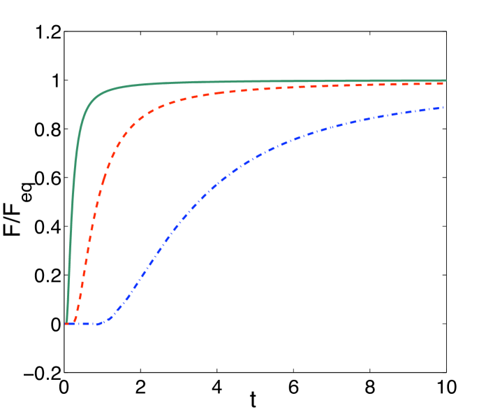
Figure 1: Approach to equilibrium for various values of the plate separation $l$ (top to bottom $l=1,2,4$) for $d=3$. Nonequilibrium force $F$, obtained by the direct numerical inverse Laplace transform of Eq. (14), plotted in units of the equilibrium pseudo-Casimir force ($F_{eq}$) as a function of time.

Now using this and Eq.(4) we find that the Laplace transform of the average value of the generalised force is given by

$$\langle{\cal L}F_{l}(s)\rangle=-{T\over 2s}\int d{\bf x}d{\bf x}^{\prime}{\partial\over\partial l}\Delta({\bf x},{\bf x}^{\prime},l)\Delta^{-1}_{s}({\bf x},{\bf x}^{\prime}),$$ (12)

which using Eq, (11) and Eq. (5) can be written as

$$\langle{\cal L}F_{l}(s)\rangle = -{T\over 2s}\int d{\bf x}d{\bf x}^{\prime}{\partial\over\partial l}\Delta_{s}({\bf x},{\bf x}^{\prime},l)\Delta^{-1}_{s}({\bf x},{\bf x}^{\prime})$$ (13)

$$= {T\over s}{\partial\over\partial l}\ln(Z(\Delta_{s}))$$

This result is quite remarkable. It means that the Laplace transform of the time dependent pseudo-Casimir force considered here is given by a static pseudo-Casimir force with the operator $\Delta_{s}$. It is clear that the result is also valid for the force on any surface in the system which interacts with the field. Providing the static partition function is known for the screened problem, the corresponding time dependent force can be extracted by inverting the Laplace transform.

We now turn to the case where the imposed boundary conditions are Dirichlet and the two plates are immersed in the fluctuating medium (hence there is fluctuating medium on both sides of each plate). For the relaxational dynamics of the field (Eq.7) we will consider the simplest case with $R=\delta({\bf x}-{\bf x}^{\prime})$, which means that the Gaussian noise is both uncorrelated in space and time. This corresponds to dynamics that does not conserve the order parameter and is also known as model A dynamics. We take the total length of the system to be $L$ which is fixed, and place the plates of area $A$ a distance $l$ apart. Standard results on the screened pseudo-Casimir interaction kar1999 give

$$\langle{\cal L}F_{l}(s)\rangle=-{2AT\over s(4\pi)^{d-1\over 2}\Gamma({d-1\over 2})}I(l,s),$$ (14)

where $d$ is the dimension of the space, $A$ is the area of the plates and,

$$I(l,s)=\int k^{d-2}dk{\sqrt{k^{2}+{s\over 2}}\exp(-2l\sqrt{k^{2}+{s\over 2}})\over 1-\exp(-2l\sqrt{k^{2}+{s\over 2}})},$$ (15)

The equilibrium behavior is easily extracted by examining the pole at $s=0$ which yields, as anticipated, the standard equilibrium pseudo-Casimir force kre1992

$$\langle F_{l}\rangle_{eq}=-{AT\Gamma(d)\zeta(d)\over(16\pi)^{{d-1}\over 2}\Gamma({d-1\over 2})l^{d}},$$ (16)

where $\Gamma$ is Euler’s gamma function and $\zeta$ is the Riemann zeta function gra2000 . The full time dependence of the force, starting at zero at $t=0$ and relaxing to the equilibrium value above, can be extracted by direct Laplace inversion of Eq. (14). Fig.(1) shows the approach to equilibrium for three different plate separations. Clearly, the relaxation times increase with plate separation and this is due to the fact that the underlying dynamics is diffusive and hence $l^{2}$ sets a time scale. Useful analytic expressions for the early and late time behavior of the non-equilibrium force can also be obtained from Eq.(14). Using specific properties of Laplace transforms and the fact that $F_{l}(t=0)=0$ allows us to arrive at an expression for the time derivative of the force

$$\langle{dF_{l}\over dt}\rangle=-{AT\over(8\pi)^{d\over 2}t^{d+2\over 2}}\sum_{n=1}^{\infty}\left[{l^{2}n^{2}\over t}-1\right]\exp(-{l^{2}n^{2}\over 2t}),$$ (17)

which in turn gives us the asymptotic behavior of the pseudo-Casimir force for different time regimes defined by $l^{2}/t$

$$\langle F_{l}(t)\rangle \sim -{2AT\over(8\pi t)^{d\over 2}}\exp(-{l^{2}\over 2t})\ \ {\rm for}\ \ {l^{2}\over t}\gg 1$$ (18)

$$\sim \langle F_{l}\rangle_{eq}+{AT\over d(8\pi)^{d\over 2}t^{d\over 2}}\ \ {\rm for}\ \ {l^{2}\over t}\ll 1$$

It is interesting to note that the late time correction is independent of $l$. This is because the medium between the two plates has a relaxation time $\tau(l)\sim l^{2}/2\pi^{2}$ whereas the slowest relaxation times in the system are associated with the medium outside the two plates and hence at late times the correction is dominated by the relaxation of the external system in the thermodynamic limit $L\to\infty$. This diffusive relaxation is responsible for the power law approach to equilibrium. It is natural to ask how these model A results translate into the stress tensor formalism. Because the rhs of Eq. (13) is static we can write the result in terms of the stress tensor for the corresponding field theory, and inverting the Laplace transform we find inprep an effective dynamical stress tensor:

$$T^{dyn}_{ij}={1\over 2}\delta_{ij}\left[[\nabla\phi]^{2}+{1\over 2}{\partial\over\partial t}\phi^{2}\right]-\nabla_{i}\phi\nabla_{j}\phi.$$ (19)

Thus for the problem considered here we see that the first part of the stress tensor picks up a time derivative term whose expectation will vanish in equilibrium to give the usual equilibrium stress tensor result. It is also clear that simply using the standard stress tensor on a surface in a system out of equilibrium will only give the right result when Dirichlet boundary conditions are imposed (as $\phi=0$ on the surface).

The method can also be used to examine the dynamics resulting from a sudden change in temperature, from say $T_{0}$ where the system is in equilibrium to a temperature $T$. In this case, the initial configuration of the field $\phi({\bf x},0)$ has the correlation function

$$\langle\phi({\bf x},0)\phi({\bf x}^{\prime},0)\rangle=T_{0}\Delta^{-1}({\bf x},{\bf x^{\prime}},l).$$ (20)

Solving the equation of motion Eq.(7) with this initial condition yields the time dependent correlation function

$$C({\bf x},{\bf x}^{\prime},t)=T_{0}\exp(-2t\Delta)\Delta^{-1}+T(1-\exp(-2t\Delta))\Delta^{-1}$$ (21)

The same reasoning as for Eq.(9)-(13) yields

$$\langle{\cal L}F_{l}(s)\rangle={T_{0}\over s}{\partial\over\partial l}\ln(Z(\Delta))+{T-T_{0}\over s}{\partial\over\partial l}\ln(Z(\Delta_{s}))$$ (22)

where we have used the fact that ${\partial\over\partial l}\ln(Z(\Delta_{s}))$ is independent of the temperature. For Dirichlet boundary conditions this gives, in analogy with Eq.(18), the limiting behavior

$$\langle F_{l}(t)\rangle \sim \langle F_{l}\rangle_{eq\ T_{0}}-{2A(T-T_{0})\over(8\pi t)^{d\over 2}}\exp(-{l^{2}\over 2t})\ \ {\rm for}\ \ {l^{2}\over t}\gg 1$$ (23)

$$\sim \langle F_{l}\rangle_{eq\ T}+{A(T-T_{0})\over d(8\pi)^{d\over 2}t^{d\over 2}}\ \ {\rm for}\ \ {l^{2}\over t}\ll 1$$

One can also consider the behavior of the pseudo-Casimir force for relaxational dynamics of the form of Eq.(7) but where the forcing noise is colored in time such that $\langle\eta({\bf x},t)\eta({\bf x}^{\prime},t^{\prime})\rangle=T\delta({\bf x}-{\bf x}^{\prime})\omega\exp(-\omega|t-t^{\prime}|)$ (so $R({\bf x}-{\bf x}^{\prime})=\delta({\bf x}-{\bf x}^{\prime})$ has the model A from). Here $T$ represents an energy scale, $\omega$ a frequency and the resulting steady state is not an equilibrium one. The average value of the force in the steady state regime can be computed using the same formalism above and we find that the correlation function of the field is given by

$$C({\bf x},{\bf x^{\prime}},\omega)=T\left[\Delta({\bf x},{\bf x^{\prime}},l)^{-1}-\Delta_{2\omega}({\bf x},{\bf x^{\prime}},l)^{-1}\right]$$ (24)

which yields

$$\langle F_{l}(\omega)\rangle={T}{\partial\over\partial l}\left[\ln(Z(\Delta))-\ln(Z(\Delta_{2\omega})\right]$$ (25)

Hence again we find that one can compute a force in a non equilibrium system from knowledge of static screened systems comment . Note that in the limit $\omega\to\infty$ we recover the white noise equilibrium result of Eq. (5). Fig. (2) shows the frequency dependence of the non-equilibrium force obtained from Eq.(25) for a two plate system with Dirichlet boundary conditions as we had before. Again $l^{2}$ sets a timescale and we see that for $\omega\gg l^{-2}$ the force, $F$ tends to the equilibrium white noise value, $F_{eq}$, as expected, while for $\omega\ll l^{-2}$, $F\ll F_{eq}$ and as $\omega\to 0$, $F$ vanishes. The inset to Fig. (2) shows how the force depends on plate separation for fixed $\omega$. Again, equilibrium behavior is recovered for large $l$ ($\omega\gg l^{-2}$), while for small plate separations the force changes qualitatively scaling as $l^{-1}$. We note that the result Eq.(25) agrees with a computation for the same system where the steady state force was computed using the stress tensor ba2003 . We finally note that our approach can also be readily extended to study the non-equilibrium pseudo-Casimir force between two small defect regions within the pairwise approximation inprep .

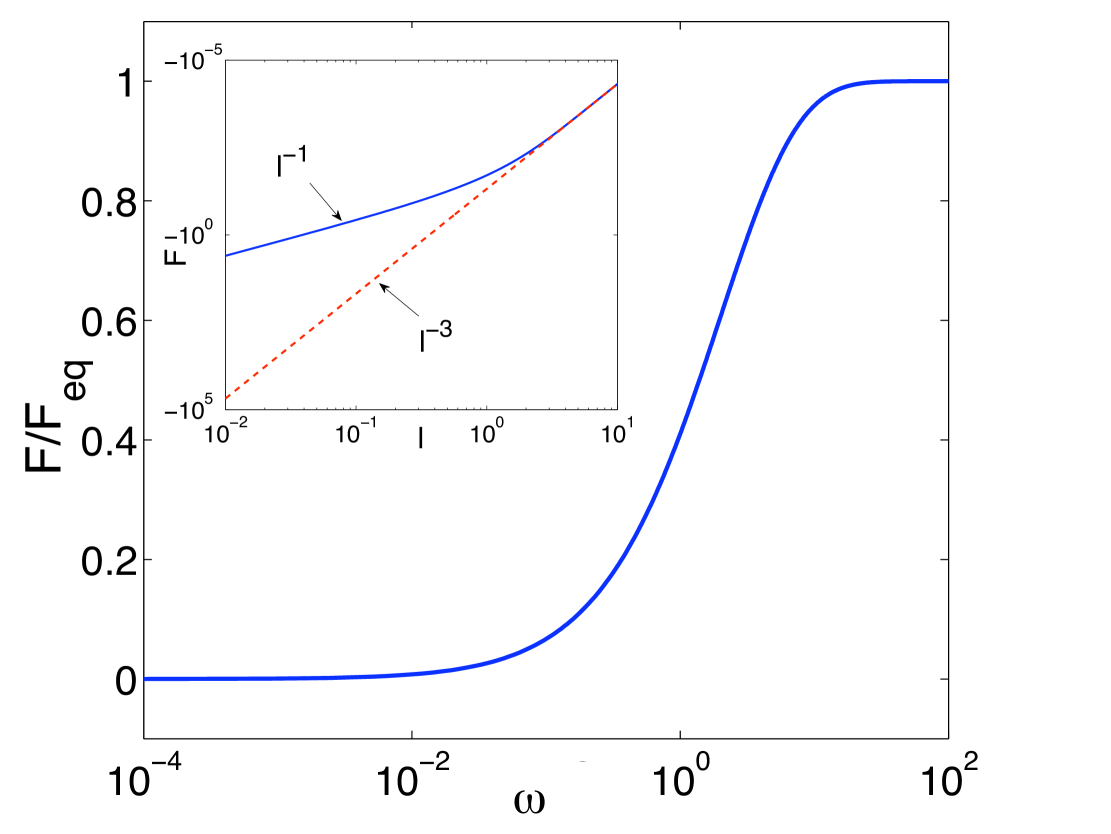
Figure 2: Nonequilibrium pseudo-Casimir force, $F$, in units of the equilibrium force ($F_{eq}$) as a function of $\omega$ for $l=1$ and $d=3$. Inset: $F$, as a function of plate separation $l$ for $\omega=1$ and $d=3$ (solid line). The equilibrium force (dashed line) is shown for comparison.

Previous studies on the dynamical pseudo-Casimir effect concentrated on steady state non equilibrium dynamics or dynamics close to equilibrium and considered Dirichlet boundary conditions assuming that the equilibrium stress tensor could be applied to compute the force. Our formalism marks a major advance that overcomes these restrictions by allowing the time-dependent force to be evaluated unambiguously via an expression for the energy of the field. We emphasize the generality of our approach as it is valid for (i) any dissipative dynamics of the form Eq. (7) , (ii) any free field theory (e.g. operators $\Delta$ which contain terms such as $\nabla^{4}$ as is the case for the height fluctuations of lipid membranes) and (iii) for any generalized force conjugate to any parameter in the system. It is worth noticing that the static theory that must be solved for conserved dynamics (model B), where $R=-\nabla^{2}$, becomes non-local and the corresponding static calculation presents us with the interesting problem of understanding pseudo-Casimir forces for systems with non local interactions. This research was supported in part by the National Science Foundation under Grant No.PHY05-51164 (while at the KITP UCSB program The theory and practice of fluctuation induced interactions 2008). DSD acknowledges support from the Institut Universitaire de France.

References

- (1) M. Kardar and R. Golestanian, Rev. Mod. Phys. 71, 1233 (1999)
- (2) V.M. Mostepanenko and N.N. Trunov, The Casimir Effect and its Applications, (Oxford) (1997)
- (3) K. A. Milton, The Casimir Effect: Physical Manifestations of Zero-Point Energy (World Scientific, Singapore) (2001).
- (4) M.E. Fisher and P.-G. de Gennes, C. R. Acad. Sci. Paris B 287, 207 (1978)
- (5) C. Hertlein, L. Helden, A. Gambassi, S. Dietrich and C. Bechinger Nature 451, 172 (2008)
- (6) R. Zandi, J. Rudnick and M. Kardar, Phys. Rev. Lett. 93, 155302 (2004)
- (7) A. Ajdari, L. Peliti, and J. Prost, Phys. Rev. Lett. 66, 1481 (1991)
- (8) D. Bartolo, A. Adjari and J.-B. Fournier, Phys. Rev. E 67, 061112 (2003)
- (9) A. Najafi and R. Golestanian, Europhys. Lett., 68 , 776 (2004)
- (10) A. Gambassi and S. Dietrich, J. Stat. Phys. 123, 929 (2006)
- (11) D. Bartolo, A. Adjari, J.-B. Fournier and R. Golestanian, Phys. Rev. Lett. 89, 230601 (2002)
- (12) R. Brito, U. Marini Bettolo Marconi and R. Soto, Phys. Rev E, 76, 011113 (2007)
- (13) M. Krech and S. Dietrich, Phys. Rev. A 46, 1886 (1992)
- (14) I.S. Gradshteyn and I.M. Ryzhik (A. Jeffrey and D. Zwillinger (eds)), Table of Integrals Series and Products, (Academic Press) (2000)
- (15) This link between the screened equilibrium Casimir force and that arising due to colored noise forcing for parallel plates with Dirichlet boundary was first noticed in ba2003 , we show here that it is a very general phenomenon.
- (16) D.S. Dean and A. Gopinathan, in preparation